Real exchange rate and innovation:
empirical evidences
Câmbio real e inovação tecnológica: evidências empíricas
KEYNIS CÂNDIDO DE SOUTO *, r MARCO FLÁVIO CUNHA RESENDE **, rr
RESUMO: O debate recente sobre os determinantes do crescimento econômico destaca o papel da taxa de câmbio real competitiva e estável para elevar o produto. Este debate tem duas abordagens: teórica e empírica. Alguns trabalhos teóricos apontam a inovação como um mecanismo de transmissão do efeito do câmbio real sobre a renda. Destacam que o câmbio real afeta o produto porque impacta diretamente os determinantes da inovação, como o investimento. Os estudos empíricos se concentram na análise da relação câmbio-produto e o link “câmbio-inovação” permanece inexplorado. Este trabalho busca contribuir para a literatura fornecendo evidências empíricas que confirmam a relação câmbio-inovação.
PAlAvrAs-chAvE: Taxa de câmbio real; inovação tecnológica; crescimento econômico.
ABSTRACT: The recent debate on the determinants of the lung-run economic growth highlights the role of a competitive and stable real exchange rate to foster growth. In this debate, the works follow two approaches: theoretical and empirical. In the theoretical approach a considerable portion of the works points towards the innovation as a transmission mechanism of the real exchange rate effects on income. These works emphasize that the real exchange rate affects growth because of its impacts on the determinants of innovation, such as investment. Despite the theoretical debate, the focus of empirical works is on the analysis of the exchange rate effects on income while the relationship between exchange rate and innovation remains untapped. This article seeks to contribute to the literature by providing empirical evidence that supports the link between the real exchange rate and innovation.
KEywOrDs: real exchange rate; technological innovation; economic growth.
JEl classification: O1.
Brazilian Journal of Political Economy, vol. 38, nº 2 (151), pp. 280-303, April-June/2018
*Universidade Federal rural de Pernambuco (Brazil). E-mail: keynis.souto@ufrpe.br.
** Universidade Federal de Minas Gerais (Brazil). E-mail: resende@cedeplar.ufmg.br. submitted: 29/
september/2016; Approved: 12/May/2017.
rKeynis c. souto thanks cAPEs for their financial support.
INTrODUcTION
From the 1980s on, several papers1 began discussing the role of the exchange
rate as a variable of long term economic growth promotion policies. The papers associate the expansion of the economic activity in emerging countries from eastern Asia (china, Taiwan and south Korea), observed between the 1950s and 1980s, to the policies of exchange rate devaluation adopted in this region, and follow two approaches: the theoretical one, with the identification of the transmission channels of the effects of exchange rate over income; and, the empirical investigation of this relationship.
rodrik (2007) highlights that market failures and weak institutions are more present in the tradable goods sector (T) than in the nontradable goods sector (NT). since the devaluation of the real exchange rate (rEr) implies the relative price raise on sector T, the consequent profit increase in this sector offset the negative effects on profit due to its market failures and weak institutions, boosting investment. The stimulus to investment on the NT sector would be lower in the presence of rEr valuation, since the profitability reduction would be lower in this sector due to market failures and weak institutions.
Bresser-Pereira and Nakano (2003) and Bresser-Pereira (2015) point out the detrimental consequences to long term economic growth in the developing coun-tries in which rEr is overvalued for a long time. According to the authors, ex-change rate overvaluation takes competitivity away from the domestic industry and leads to current account deficits, besides the replacement of domestic savings with foreign savings, without giving rise to investment increase and, thus, fostering growth. The increase of the country’s external liability caused by this scenario generates exchange rate crises with negative effects on growth.
Based on Bhaduri and Marglin (1990), Gala (2008) has demonstrated that an undervalued currency can contribute to investment and capital accumulation. According to Gala (2008), the expansion of sector T speeds up growth because the
firms in this sector are more dynamic and subject to increasing returns to scale, contributing more to innovation and to productivity increase than NT sector firms. Besides, by stimulating the most dynamic sector whose products are more technol-ogy-intensive and in which the learning-by-doing process and the accumulation of technological progress are superior, exchange rate devaluation promotes structural changes in the whole economy and leads countries in a growth and sustainable development path (woo, 2004; rodrik, 2007; Gala, 2008).
To Míssio (2012) an underdevalued rEr reduces wages share and raises
prof-it share on income, enhancing the firms’ self-financing capability. This relieves the
1 Dollar (1992), razin and collins (1997), rodrik (2007), Gala (2008), Eichengreen (2008), campos
finance scarcity problems which in turn inhibit research and innovation investments (r&D), in particular in developing countries, and it stimulates technological prog-ress which is an important source to long term growth.
campos and resende (2009) elaborate an argument based on the Evolutionary and Post Keynesian theories to demonstrate that an undervalued rEr induces a process of circular cumulative causation in which technological progress occurs in increasing rates. This process reinforces, therefore, the economic drive initially given to growth by the rEr devaluation.
In addition to a competitive exchange rate, the volatility control of the rEr is also highlighted by campos and resende (2009) as a strategy to stimulate growth through its effects over the innovation process. Furthermore, the bigger the degree of uncertainty about exchange rates is, the more unpredictable the profit margin becomes and this negatively affects investment (Atella et al, 2003; Araújo, 2009). To Aghion et al. (2006), the main consequence of this uncertainty is to spend reduc-tion with research and development by firms, which are important for long term growth.
volatile exchange rate also generates uncertainty about export revenues, reducing trade volume (hOOPEr and KOhlhAGEN, 1978; cArMO and BITTENcOUrT, 2013). The international trade is important because it leads firms to increase their productivity and their efforts to innovate. Thus, a stable exchange rate fosters effi-ciency, productivity and growth (Biesebroeck, 2005; schnabl, 2007).
Therefore, authors such as Aghion et al. (2006), Míssio (2012), campos and resende (2009), Gala (2008), among others, point to the exchange rate-innovation-growth relationship. however, the transmission channels between exchange rate and innovation are still underexplored in the theoretical literature about exchange rate and growth. The papers have been focusing on the link between the exchange rate and growth and, generally, they conclude that a real competitive and stable
exchange rate affects long-run economic growth2. The aim of this paper is to
con-tribute to the literature providing empirical evidence of the real exchange rate-in-novation relationship.
In what follows, we begin in the second section by presenting an Evolutionary/ Neo-scumpeterian model for innovation in which innovation is determined by the rEr. The third section presents the methodology used to test the hypothesis of the exchange rate-innovation relationship. The results are on the fourth section and confirm the hypothesis of the effect of exchange rate over innovation. The last sec-tion summarises and concludes.
2 Dollar (1992), razin e collins (1997), rodrik (2007), Gala (2008), Eichengreen (2008), Míssio (2012),
EvOlUTIONAry APPrOAch AND ThE INNOvATION DETErMINErs
On the Evolutionary theory, innovation is a result of a wide array of factors which act both on the individual firm scope and on a systemic scope. Therefore, the development of a model that considers all the determinant factors for innovation is not trivial and the simplification of this reality (production of innovation) by means of a single-equation model must be made with due caution on the risk of losing relevant aspects of the “innovation” phenomenon. Nevertheless, and recog-nizing the likely limitation of such simplification, the goal of this section is to propose a model that considers the innovation determinants (considering specifi-cally the “systemic dimension” of this process) and that can be used to analyse the link between exchange rate and innovation.
In the systemic scope, innovation results from a process that involves all the economic and social environment in which the “key innovator agent” is inserted (Freeman, 1995, 2002; Dosi et al, 1994). Two factors are fundamental in this pro-cess: knowledge increase and learning, both made viable by the interaction and the information flow among the agents that act in the environment (lundvall, 1988; Albuquerque, 1996). From this Evolutionary/Neo-schumpeterian perspective three main factors can be highlighted as determinants of innovation by affecting the in-formation flow and the interaction between the agents and, consequently, knowl-edge and learning:
i) The Investment on Physical Capital (I) – considered as a “necessary factor,
though not sufficient”, to innovation and technological progress. According to Dosi et al. (1994), the investment on fixed capital is essential to the successful diffusion of new technologies and provides learning to the agents because technology is
embedded into machines and equipment3. If this technology acquisition from
invest-ment (gross fixed capital formation) is accompanied by adaptation and perfection-ing efforts (in contrast to the simple “use” of the technology), the investment can have positive effects over learning (learning-by-doing) and, consequently, over in-novation (Dosi et al., 1994; Freeman and soete, 1982). Thus, it can be expected that the bigger the physical capital (I) investment is, the greater will be the innova-tion (IN):
!!"!! ! ; !!!!! (1)
ii) A Path Dependence or Cummulativity (CC) – refers to the Evolutionary
idea in which technological change or the “evolution of innovation” is conditioned by its own history – the result of today’s basic and/or incremental innovations set
3 To Dosi et al. (1994), some technologies can be acquired or transferred without the need of investing
a higher standard for the success of tomorrow’s “innovative” efforts. This process occurs because each new technology enables an increase in knowledge and at the same time it depends on the level of accumulated knowledge. The more accumu-lated knowledge (cc), the greater are learning and innovation. This has to do with the indivisibility of knowledge and the incremental nature of learning (Nelson and winter, 1982). Thus, It can be defined that:
!"!! !! ;
!"!! !!!!!!!!!!!!! !!!! (2)
iii) The National Innovation System (NIS) – The concept of NIs is crucial for
understanding the “systemic determinants” of innovation. For the Evolutionaries, the innovation process is directly related to this concept. According to Albuquerque (1996), a country’s NIs is an institutional structure that results from a planned conscious action or from the sum of non-planned disjointed decisions. Through the construction of the NIs, the “agents” of the environment (social and economic) that play a fundamental role to the development of innovations are identified; and, the role of each agent in this system is established, in other words, the “institutional division of labor” is established (Bernardes and Albuquerque, 2003; ribeiro et al., 2006). however, the identification of the agents and their respective function with-in the chawith-in of a country’s with-innovation is not all that characterizes the NIs and de-fines it as a determining innovation factor. As Bernardes and Albuquerque (2003) highlight, this social system is crucial for innovation because it enables interaction and mutual feedback between the institutions, which leads to a wide definition of NIs – a social system (whose central activity is learning, which involves interactions between people) that is dynamic (characterized by positive feedback and reproduc-tion), whose “elements” mutually reinforce each other. Moreover, in the NIs, po-litical, institutional and cultural influences, as well as economic policies affect the innovation’s success (lundvall, 1992; Freeman, 2002). The interactions and feed-backs allow greater information flow and an increase in scientific and technical knowledge, which are fundamental to generate innovation and technological prog-ress. Thus, the NIs “summarizes [...] the processes that translate innovation and imitation into economic growth” (ribeiro et al., 2006, p. 81).
of multilateral trust relations can be established (lundvall, 1992; lundvall et al., 2002). This environment is present in the NIs context.
Thus, the NIs eases communication by enabling the interaction of “environ-mentally similar agents” and makes greater information fluxes viable. Beyond fa-cilitating communication, lundvall (1992) states that the actors that compose the NIs influence the quality and quantity of the information in a fundamental way, besides acting in the organization of this information, easing interchange and boost-ing knowledge, innovation and technological progress.
These effects will be greater the more developed (or mature) the NIs is. The interaction and feedback channels are completely formed, strong and involve a bigger number of agents in mature NIs (Bernardes and Albuquerque, 2003; rIBEIrO et al., 2006; Albuquerque, 2009). consequently, the interaction and in-formation flow will be greater and so will the innovation production.
The NIs literature points to a structure composed by a wide array of institu-tions involving firms, universities, research instituinstitu-tions, the government, scientists’ and engineers’ activity, which are articulated with the educational system, with the industrial and corporate sector and also with financial institutions, completing the circuit of the agents that are responsible for generating, implementing and dis-seminating the innovation.
Despite this broad array of institutions that shape the NIs and affect the in-novative performance of a country, it is acknowledged in this paper that at least three agents are essential to the development of the NIs: The firms – locus of in-novation and r&D (Dosi et al., 1994; Nelson, 1996); the educational and research institutions (Especially universities) (Freeman, 1995); and, the government – eco-nomic policy and institutions are central in innovation process (Freeman, 1995). These agents’ actions on the NIs and their effect over innovation happens through three main factors: research and development (r&D), education (educ) and eco-nomic policies (EP). Thus:
!"!! !"#$!!!!!!" , (3)
being: or !!!"#$ !!!!!!!!!!!!!!!!!!!"!! 0 or !!!!" !!
Therefore, it can be established that on the Evolutionary perspective the sys-temic determinants of technological innovation involve the aggregate investment (I), the accumulated knowledge (cc), education (educ), research and development (r&D) and the economic policies of the government (EP). This can be represented by the following function:
!"!!!!!!!!!!!"#$!!!!!!!!"! (4)
each other. when it comes to economic policy (which involves fiscal, monetary, exchange rate, commercial, regulatory, credit policies and so on) it can have a positive or negative effect over innovation4.
The goal of this study is to analyse specifically the effect of foreign exchange policy over technological innovation. Aiming to simplify the model to make it operational, enabling its estimation, the variable EP will have the level of the real exchange rate (rEr) and its volatility (vrEr) as proxies, both of which are con-sidered as fundamental to determine economic growth through effects over tech-nological innovations in the recent literature. replacing these two factors in (4) the following equation for the systemic innovation determinants can be expressed by:
!!!!!!!!!!"#!!!!!!!"!!!"#"!5, (5)
Aghion et al. (2006), campos and resende (2009), Míssio (2012), Gala (2008), carmo and Bittencourt (2013), among others, indicate, by means of different chan-nels, the positive effects of the exchange rate and its stability, over innovation. Thus:
!!!!"!!! 0; and, !!!!"#"!!.
EMPIrIc MODEl AND METhODOlOGIcAl PrOcEDUrEs
In order to statistically analyse the exchange rate-innovation relationship as defined in equation (5), a panel data method was used and the following empirical model was defined:
!"#$!"!!!!!"#!"!"!!!!!!!"!"#!"!!!!"#$%&!!!!"!!!!"
!!!!"#$!!"!!!!!!!"#"!"!!!"! !"#$!"!!!!!"#!"!"!!!!!!!"!"#!"!!!!"#$%&!!!!"!!!!"
!!!!"#$!!"!!!!!!!"#"!"!!!"!
!"#$!"!!!!!"#!"!"!!!!!!!"!"#!"!!!!"#$%&!!!!"!!!!"
!!!!"#$!!"!!!!!!!"#"!"!!!"!
(6)
where: INitis the technological innovation (in the i-th country and at period
t) measured by the number of patents (Utility Patents – “patents for invention”);
INit-1 is a “proxy” for accumulated knowledge (cc); INVit is the physical capital
4 For example, the purchasing policy of the government towards technology-intensive sectors has a
positive effect on innovation. conversely, tax policy has an indirect effect: an elevation of taxes that levy over profits of the innovative firms discourages innovation while reduction or exemption of the taxes on r&D related expenses encourages innovation.
5 The objective here is to analyse the statistic relationship among these variables using the econometric
measured by the Gross Fixed capital Formation (GFKF) as a proportion of the
GDP; EDUCit is education measured by the percentage of the population with
higher education; R&Dit represents expenses with research and development
mea-sured as a proportion of the GDP; uit = ai + eit is the compound error term of the
model, being eit the random disturbance (captures the impact of non-observed
factors over the dependent variable) and ait a random variable which captures
heterogeneity or the non-observed characteristics, specific to each country, that
affect innovation; RERit is the indicator of the real exchange rate misalignment;
and, VRERit is the volatility of the exchange rate.
The real exchange rate misalignment indicator (RERit) was calculated
follow-ing rodrik (2007). For the exchange rate volatility (VRERit), two measures were
chosen: the Perée and steinherr (1989) measurement and the mobile standard de-viation (MsD), named, respectively, as vPs and vsD, using “windows of
observa-tion” of 3 to 5 years (resulting in four measures vPs3, vPs5, vsD3, vsD5)6. The
database for these indicators was Penn world Table (8.0). To measure patent vari-ables, GFKF/GDP, education and r&D, the data was obtained from the United states Patent and Trade Office (UsPTO) website and from the world Bank (world Development Indicators).
On the specification of equation 6, two aspects related to the measurement of the variables require explanation. First, the use of INit-1 as a proxy for the
accumu-lated knowledge variable (CCt) – a variable which affects innovation and cannot
be directly observed – is based on the evolutionary presupposition of path depen-dence (innovation conditioned by its own history) and on the idea that in each innovation (radical or incremental) that happened at the t-1 period, more
know-ledge is generated for the t period (CCt)) and it accumulates for the innovation
round on period t (INt).
The second aspect refers to the patents as a measure for innovation. The com-plexity of the innovation concept points to the difficulty in measuring this variable. Innovation is a multidimensional process and involves the creation of something qualitatively new (to the firm or to the economy) and marketable, it can result on new products or processes, on the amplification of capabilities and competences, on the increase of knowledge, etc. Therefore, the main problems with measuring innovation come from the basic conceptualization of the object meant to be mea-sured, from its ability to measured and to the possibility of having different kinds of measurement (smith, 2005). As an alternative to these problems, the patent
data are being used as an indicator of technological innovation7.
however, this indicator presents a few limitations that need to be properly
6 These measurements have been utilized in several papers. For further detail, Perée and steinherr (1989)
servén (2002), clark et al. (2004), Aghion et al. (2006), schnabl (2007), Bittencourt, larson and Thompson (2007), Araújo (2009), calderón and Kubota (2009), Mukhtar and Malik (2010).
7 That is what can be observed in Bernardes and Albuquerque (2003), ribeiro et al. (2006), herskovic,
considered while using it to measure innovation. The most notable one, according to smith (2005), is that the patents “determine” the emergence of a “new technical principle” and not of commercial innovation. In this perspective, the patent data represent more of an invention indicator than one of innovation per se. Kleinknecht et al. (2002) apud smith (2005) point out that some inventions and innovations are never patented and many patent requests will never be commercialized. Bernardes and Albuquerque (2003, p.873), further highlight two limitations to the patent data from UsPTO. “[...] from commercial linkages with the Us to the qual-ity of the patent: [...] local innovation necessarily is limited to imitation in the initial phases of development, and imitation or minor adaptations do not qualify for a patent in the UsPTO”. Therefore, patents don’t always represent a perfect measure for innovation. however, for the authors, taking such limitations into ac-count and considering their implications for the quality of the results, the use of patents has been shown to be very useful to research with innovation. This data has the advantage of gathering relatively continuous information about new tech-nology and make them available to the public for a prolonged period, enabling long term research. “This gives it striking advantages as an innovation-indicator” (smith, 2005, p. 158).
On the estimate of equation (6), two important points must be observed: the necessary time for the changes in the explanatory variables to manifest in variations of innovation; and, the problem of endogeneity. It is known that the innovation production is a long term process in such a way that the impact of changes in the innovation explanatory variables occur with some time lag. A way of dealing with this issue, which is common in the literature that investigates empirical long term relationship between economic variables, is to use a simple five-year average of the observed variables.
In this study the database covers the period of 1996 a 2010 (T=15 years) and was defined by the restriction of information availability for some variables, main-ly r&D. Due to this limitation, three-year simple averages were used, so that the 15 years were converted in five periods of three years (from t1 = 1996-1998 to t5 =
2008-2010). In this case, the estimates parameters (g and b’s) indicate how
chang-es in the explicative variablchang-es, which happened over a period of three years, affect innovation in this period.
The endogeneity of the explicative variable implies the presence of correlation between the regressive factors (Xit’s) and the error term of the model (uit), E(Xit uit)
≠ 0 leading to inconsistent measures for the parameters (g e b’s) when estimated by Ols. On equation (6) there are three possible sources of endogeneity: i) the dy-namic effect – lagged dependent variable (INit-1) is correlated to the error uitdue to
the presence of individual unobserved effects, even though it is assumed that it isn’t autocorrelated; ii) the issue of omitted variables such as economic policies (mon-etary, fiscal, etc.), which affect innovation (the dependent variable) and the explica-tive variables education, (EDUC), investment (INVit) and r&D; in addition to the possibility that there are specific characteristics of the countries – captured by (ai)
consequently, innovation8; e, iii) the simultaneity – happens when at least one
ex-plicative variable is determined simultaneously with the dependent variable. It is what can be assumed for investment (INVit) and innovation (INit)9.
To deal with the endogeneity problem, the model was estimated using the
GMM-system in two stages (considering the variables INit-1, INVit,, EDUCcit e
R&Dit as potentially endogenous and the variables RERit and VRERit as
poten-tially exogenous) and robust for heteroscedasticity10. A fixed cross-sectionally
dominant panel was used, composed of 76 countries, not balanced in the temporal aspect, but with a low amount of missings (2%).
The estimator “GMM-system two-step” from Arellano and Bover (1995) and Blundell and Bond (1998) uses Instrumental variables and the Generalized Method of Moments (GMM) and allows for consistent estimates of the parameters. The two-stage estimate consists in estimating the parameters g e b’s of the equation (6) through a system that combines two equations:
!"!" !!!!"!"!!!!!"!!!!!!!!" (7)
!!"!" !!!!!!"!"!!!!!!!!"!!!!!!!", (8),
using (!!"!!!!!!!!"#$!!!!!!!!"#!!!!!!!!!!!"!!) as instruments for the
endoge-nous variables in the estimation of the level equation (7); and the lagged explicative variables(!"!"!!, !"!"!!, !"#$!"!!!!"#$!"!!!!"#!"!!!!"#!"!!!!!!"!!! !!!!"!!) as
in-struments for the equation in first difference11.
The robustness of the estimation using the GMM-system depends on the valid-ity of these instruments. The hypothesis is that they are orthogonal (exogenous). Three validation tests were applied to the estimated model: the sargan/hansen test; the Difference-hansen test and the residue autocorrelation by Arellano-Bond (1991).
8 This corresponds to specifying the model given by equation (6) as a model of fixed effects. According to
Marques (2000, p. 24), this choice is more appropriate “when the sample is relatively aggregated (i.e., at levels of regions, countries, etc.) and the goal of the study is not the prediction of individual behavior [...]”.
9 It is understood that this simultaneity between (INvit) and (INit) does not occur at the same moment
in time (t) as is highlighted by romero (2011, p. 110). For the author, it is likely that the simultaneity between investment (on t) and innovation (on t) will hardly be found “since the investment would only significantly impact innovations with some time lag”. however, by defining t as a three-year period, it is possible to assume double causality between innovation and investment.
10 The command xtabond2 was used on stata 12.0 which applies, automatically, the windmeijer’s
correction (2005) for the standard deviation bias of the two-step estimates, on small samples. More details in roodman (2009).
11 The proposition is to use a delay or at least two periods (2 lags) x
it-2 as an instrument for each
endogenous variable ∆xit and, for a large or moderate time dimension (T), a maximum delay of four
periods xit-4 (cameron and Trivedi, 2005). In this paper, to avoid the proliferation of instruments that
The “sargan/hansen test” examines the joint validity of the instruments. The hansen test (robust for heteroscedasticity and autocorrelation problems, but
weak-ened in case there are many instruments), tests the null hypothesis (H0) of the
or-thogonality of the instruments; and, the sargen test (not robust, although stronger relative to the proliferation of instruments) tests the null hypothesis (H0) that the
instruments of GMM-sys are correlated to the errors. The acceptance of H0-hansen
and the rejection of H0-sargan confirms the validity of the instruments that were
used. The “Difference-hansen test” examines the joint hypothesis that both the level equation instruments and the difference equation instruments are exogenous and is a complementary test to the “sargan/hansen test”.
The third important test to confirm the robustness of the model is the one by Arellano-Bond (1991) for serial autocorrelation of the residues eit. In the model for
innovation the error term has two components: uit = ai + eit. The term uitis, by
defi-nition, autocorrelated because it contains fixed time effects (ai), but the GMM-sys
eliminates this correlation source. however, as roodman (2009) highlights, if eit is
serially correlated (E[!!"!!"!!!!!"#!!!!!!!!"!!!!!!!), some level variable lags become invalid instruments for the first difference model.
In the model for innovation, if eit shows first order serial correlation, so:
E!!!!!!!!!! !! and !!!!!!!!!!!!!! !!. In this case, !"!"!!, !!!"!"!!, !"#!"!!, and !!!!!"!! stop being valid instruments for the first difference equation, because they will be endogenous to the error term !!!"!!!!"!!!!!!!! by way of ei,t–1. The Arellano-Bond
test (1991) is done over the first difference residue (∆eit ), under the null hypothesis
that there is no autocorrelation of first (!!!) and of second order (!!!). The most
important result to confirm the validity of the instruments is the acceptance (or non-rejection) of(!!!). This guarantees sufficient conditions to confirm that the
instruments used are valid.
Beside the overidentification tests, an additional “test” was performed to
con-firm the elimination of the “dynamic panel bias” and the consistency of the
GMM-SYS estimator, following the proposal of roodman (2009) and Bond (2002). These
authors suggest the use of the Within and OLS estimator, which provide biased
estimates (Within underestimates and OLS overestimates) for the
g
^ parameter(Dynamic test coefficient ini,t-1). Thus, good estimates of the true
g
parameter, using GMM-SYS, must be within the limits of the Within and OLS estimates.ANAlysIs AND rEsUlT DIscUssION
Before estimating equation (6), which shows the relationship between the real exchange rate (level and volatility) and technological innovation, the following
specification tests were applied for the panel data: The F test (Chow’s test), the
Breusch-Pagan test (LM:Lagranger-multiplier), and the Hausman test12.
The F and lM tests confirmed the existence of individual effects (or
heteroge-neity) that weren’t observed in the panel and the Hausman test confirms that the
fixed effects model is the most efficient one. Therefore, the specification of the dynamic model for innovation as a fixed effects model is the most adequate one. In addition, to investigate robustness, two measurements were used for the volatil-ity of the real exchange rate: moving standard deviation (vsD3 e vsD5) and P&s (vPs3 e vPs5); and, as proposed by Bond (2002) and roodman (2009), to analyse
the efficiency of the estimator GMM-SYS in the elimination of the bias, the
equa-tions were also estimated by OLS and Within. however, the presentation and
analysis of the results focuses on the estimates using GMM-SYS e vPs5.
First, through the estimation of the equation (6), the hypothesis that an under-valued and stable exchange rate stimulates innovation was tested.
!"#$!"!!!!!"#!"!"!!!!!!!"!"#!"!!!!"#$%&!!!!"!!!!"
!!!!"#$!!"!!!!!!!"#"!"!!!"! !"#$!"!!!!!"#!"!"!!!!!!!"!"#!"!!!!"#$%&!!!!"!!!!"
!!!!"#$!!"!!!!!!!"#"!"!!!"!
!"#$!"!!!!!"#!"!"!!!!!!!"!"#!"!!!!"#$%&!!!!"!!!!"
!!!!"#$!!"!!!!!!!"#"!"!!!"!
In this equation, the parameters g, b1, b2, b3 e b4 measure individually the par-tial elasticity of innovation in relation to the percentage changes in the respective variables: INit–1, investment, education, r&D and rEr – all of which expressed in
natural logarithm. The b5 coefficient measures the “semi-elasticity” of innovation
relative to the volatility of the real exchange rate – it indicates what is the expected percentage change in innovation, when vrEr varies in a single unit. The goal is to investigate the hypotheses that: i) b4 > 0 – the undervaluation of the real exchange rate stimulates innovation; and, ii) b5 < 0 – a volatile real exchange rate discour-ages investment in innovative actives. The results of the estimation of this model are at Table 1.
Analysing the quality of the estimation initially, the tests show that the results are statistically robust: the Arellano-Bond test of absence of autocorrelation of the residue has the result that confirms the validity of the instruments and the estimates (rejects !!! and doesn’t reject !!!); the sargan/hansen test, rejects H
0-Sargan and
does not reject H0-Hansen confirming the orthogonality and the validity of the
instruments used; and, the Difference-Hansen test also confirms that all the
instru-ments are valid (the instruinstru-ments are not correlated with the error). Furthermore, the estimated value for
g
^ (coefficient of the dynamic variable int-1) can be foundbetween the limits of the values estimated by Within (which underestimates) e OLS
(overestimates), highlighting the fact that GMM-SYS provides a good estimate and
manages to eliminate the bias in the dynamic panel.
The results show that all the estimated parameters of the model, with the excep-tion of !!
!! and !!
(which captures the effect of education over innovation), are statistically significant and have the expected signs. The
g
^ parameter which captures the effect of accumulated knowledge (int-1) over technological innovation is significant at 1% and shows that, for each 10% increase in innovation production in t-1, there is an in-crease of around 6% in the innovation in t. The parameters!!
!! and and !! !!
!! and !! which capture,
over innovation, are significant at 10% and 5%, respectively. These results indicate that for each 10% elevation of the investment in the period of three years it is pected for innovation to increase in 4,5% within this same period and, for the ex-penses with r&D, an increase of 10% in it stimulates a 6,9% innovation growth.
Table 1: Dynamic Model for Innovation (Equation 6)
Explanatory variables
GMM-SYS two step
Coeficients robust-SD p-value
int-1
^
g = 0,6038 0,1424 0,000*
inv b^1 = 0,4486 0,2400 0,066***
educ b^
2 = 0,3076 0,2244 0,175
r&d b^3 = 0,6889 0,2949 0,022**
rer b ^
4 = 0,2711 0,1367 0,051***
vrer(vps5) b^
5 = - 0,4743 0,9880 0,000*
Constant b^0 = 1,4594 1,1143 0,195
Instrument Validation Tests (significance level of 5%)
Arellano-Bond Test !!!
: absence of serial correlation AR(1) !!!: absence of serial correlation AR(2)
p-value 0,001 0,101
Sargan Test
H0: non-orthogonal additional instruments
0,019
Hansen Test H0: orthogonal instruments
0,139
Difference-Hansen Test H0: all the instruments are valid H0: additional instruments are exogenous
0,371 0,80
Dynamic panel bias elimination test (estimates for g)
Within 0,1663 (p-value = 0,016)
GMM-SYS 0,6038 (p-value = 0,000)
OLS 0,9316 (p-value = 0,000)
Countries 76
Observations 380
Instruments 22
Source: Own elaboration based in the regressions.
Notes: * significant at 1%, ** significant at 5%, *** significant at 10%.
the education variable is not an important determinant of technological progress. Actually, Evolutionary/Neo-schumpeterian literature confers great importance to
education in the development of innovation and technological progress. Freeman (1995) emphasizes that list already pointed in 1841 to the relevance of the educa-tion system for the introduceduca-tion and diffusion of new technologies. The author argues that social changes done is the Eastern Asian countries, such as the agrarian reform and universal education, explain, among other factors, the magnitude of the technological and structural changes observed in those countries, and points to the difference between the education systems of south Korea and Brazil as one of the factors that explain the different economic performance that these countries had over the last few decades (Freeman, 1995, p. 14). rosenberg (2000) show the key role of the American universities for the development of science and technological knowledge, the emergence of new technologies or industries, the diffusion of tech-nologies and the remodelling of the structure and the performance of the American economy, as well as, the linkages between universities, the private sector and gov-ernment. “I conclude that American universities have been especially successful as producers of economically useful knowledge” (rosenberg, 2000, p. 57). Albuquerque (1996, p. 228), defines the National system of Innovation as “[...] an
institutional construction that drives technological progress [...] institutional ar-rangements that are articulated with the education system, with the industrial and corporate sector, and with financial institutions, making up the circuit of agents that are responsible for generating, implementing and dissemination of techno-logical innovations”. Therefore, rigorously speaking, in statistical terms a
non-significant b^2 allows one to only conclude that evidences were not found of the
causality between education and innovation, for the assessed group of countries and the period, but it is not possible to generalize and state that education doesn’t affect innovation. The result can be a consequence of the proxy used to measure the education variable (percentage of the population with higher education). This measure was chosen for being available in a big amount of countries in the analysed period13.
The variables of greatest interest in the regression of equation (6) are those
which capture the effect of devaluation (RER) and of volatility (VRER) of the real
exchange rate over technological innovation. The estimated coefficient for the vari-able RER (b^4 = 0,2711) is significant to the level of 10% and has the expected sign. This result indicates that an increase (devaluation) of 10% in the real exchange rate
13 Nonetheless, innovating requires continuous knowledge and learning. Part of the ability to acquire
over the period of three years, leads (ceteris paribus) to an expected increase in innovation of about 2,7%, in the same period.
with regard to exchange rate volatility (VRER), its coefficient has been shown
to be significant to the level of 1% with the expected sign, and it indicates that a 10% reduction in exchange rate volatility increases innovation in about 7,9% over
the same period14. The effect of exchange rate volatility over innovation is
con-firmed (with robust results considering significance levels of 5% and 10%), even when the model is estimated using different measurements of volatility (vPs3, vsD5
e vsD3), with some changes to the magnitude of the estimated coefficients15. These
results corroborate the hypothesis that the devaluation of rEr and its volatility have effects on innovation and technological progress, for the period and group of countries that were analysed.
Following the Evolutionary perspective, one of the main hypothesis we ad-opted to explain the exchange rate-innovation relationship is the effect of exchange rate over a fundamental input to produce innovation that is the information flow, and over the decision to invest of the agents. The devaluation of the real exchange rate, by boosting profitability and stimulating production, exports and investment in the tradables goods sector (T), increases the information flow, fostering the
in-crease of knowledge and learning of the agents in the sector16. According to rodrick
(2007), the T sector show more market failures and weaker institutions than the nontradables goods sector (NT). In addition, the author also highlights that sector T has more complex productive chains with great circularity relative to the produc-tive chains of the NT. As a consequence, producproduc-tive chains on sector T show intense labor division among firms and greater number of interactions among agents in the various steps of the productive process, than the chains of the NT sector. The high degree of circularity and complexity of the productive chains of sector T boosts the information flow among the agents, acting as a stimulator of technological progress and of the technological spill over.
Finally, williamson (2003) argues that an undervalued real exchange rate raises the relative prices of T goods, but does not reduce aggregate demand, because the market of T goods is proportional to the size of the global economy. Due to
14 The way it was defined in the model, the estimated coefficient for vrEr (^
b5 = – 0,4743) measures
the expected percentage change in innovation, when vrEr varies in one unit. here, it was chosen to
interpret the results in terms of elasticity – expected percentage variation in innovation when vrer
increases (or decreases) by 10%. To obtain this elasticity, the estimated coefficient for ^
b5 = – 0,4743 is
multiplied by the medium value of the used volatility measurement E(vps5) = 1.676 obtaining
∆%in = – 0,795 (∆%vcr).
15 For estimates using vsD5, for example, the estimated coefficient for vrer was ^
b5 = – 3,4855 and
E(vdp5) = 0,084. Thus, the elasticity of innovation relative to the volatility captured by this measurement is (0,293) indicating that a 10% increase in volatility reduces innovation in about 2,9%. The results using the measurements (vPs3, vsD5 e vsD3) can be found in Annex 2.
16 The information flow can be considered as the “trigger device” of innovation and the devaluation of
the real exchange rate can be seen as a “trigger device” and an “amplifier device” of the information
these factors (more market failures, weaker institutions, more complex production chains with great circularity and the size of the market of the T goods) an under-valued rEr leads to greater investment growth rates, economic activity and, there-fore, information flow on sector T than an overvalued rEr causes in the NT sector. consequently, in contrast with the appreciation of the rEr, its devaluation stimu-lates innovation in the economy as a whole.
On the other hand, it is argued that there is a negative correlation between the rEr volatility and the production of technology. The more volatile the rEr is, the greater the uncertainty about profitability will be in the sector of T goods, inhibit-ing investment and economic activity in this sector. The decrease of the economic activity in the sector T segments which are technology and knowledge intensive mitigates the information flow among the various links of its productive chains, destructuring the “built innovative capabilities” in the sector T firms, with deleteri-ous effects on investment in innovation and technological progress.
however, a necessary condition for the positive impact of a stable and under-valued rEr over the information flow and increases in the knowledge, learning and innovation in a given country, is the presence of a developed National Innovation system (NIs). The NIs fosters and potentiates the information flow in the innovation chain, because it enables interactions and mutual feedback among the “key-agents” of the process. The more developed (or mature) the NIs is, the greater is the interaction among these agents and the greater the information flow among them will be. This happens because in a mature NIs the interaction and feedback channels are completely formed, stronger and involve a great number of agents (firms, universities, research institutions, government, engineers, scientists, etc.). consequently, greater will the innovative capabilities and the innovation pro-duction be. Thus, the effect of a stable and undervalued rEr over innovation will be different when comparing countries with mature NIs to those in which NIs is underdeveloped. Two hypotheses can be highlighted for this “Exchange rate-NIs-Innovation” relationship:
i) The effect of the rEr devaluation over innovation will be greater in
coun-tries with mature NIs vis-à-vis to those with NIsin catching up and non-mature
NIs. This happens because, in the mature NIs, the interaction channels involve a bigger number of actors and all the connections are “working”. Thus, the informa-tion flow in these systems are greater and consequently learning will be greater in
the innovation chain of the“tradables firms”, potentializing the effect of real
ex-change rate over the introduction of innovation; and,
ii) The effect of the rEr volatility disorganizing the channels of interaction in the tradable goods productive chain and disrupting the information flow and, con-sequently, discouraging innovation, is lesser (is smoothened) in countries with a
mature NIs vis-à-vis to those with a catching up NIs and a non-mature NsI. This
they present greater robustness on the financial and market position aspects. These factors make the firms on the T sector less sensitive to the income reductions caused by a volatile rEr, attenuating the negative effects of exchange rate volatility over the innovative activities in these firms. These two hypotheses were tested estimating the following equation:
!"#$!"!!!!!"#!"!"!!!!!!!"!"#!"!!!!"!"#$!"!!!!"!!!!"
!!!!"#$!!"!!!!"#"!"!!! !"!!!"#
!!! !"#"!!"# !!!!!!"
!"#$!"!!!!!"#!"!"!!!!!!!"!"#!"!!!!"!"#$!"!!!!"!!!!"
!!!!"#$!!"!!!!"#"!"!!! !"!!!"#
!!! !"#"!!"# !!!!!!"
!"#$!"!!!!!"#!"!"!!!!!!!"!"#!"!!!!"!"#$!"!!!!"!!!!"
!!!!"#$!!"!!!!"#"!"!!! !"!!!"#
!!! !"#"!!"# !!!!!!"
(6’)
In which: NIs is a dummy whose values are defined NIs = 1 for countries with
a mature NIs and NIs = 0 otherwise; (rEr x NIs) and (vrEr x NIs) are
interac-tion variables which capture the joint effect of exchange rate devaluainterac-tion and ex-change rate volatility in countries with a mature NIs, respectively, over innovation. The construction of these dummies had as a reference the work of Bernardes and Albuquerque (2003), ribeiro et al. (2006); herskovic et al. (2008) and Albuquerque (2009). Using a technique called “super-paramagnetic”, these authors
have grouped the countries according to different development levels of their NIs’s. The countries were classified in three schemes: scheme I includes countries in which the connections among the NIs agents do not exist or are very weak; in scheme II are the countries that do not posses a complete NIs (or mature); in this scheme, the links among the NIs agents exist, but are weak; and, in scheme III are the countries in which the NIs is well developed (mature) so that all the connections are “work-ing” and are strong. Thus, on the definition of the interaction dummies, NIs = 1 for
countries in scheme III (mature sI) and NIs = 0 otherwise17.
By estimating the coefficients of equation (6’) the goal is to test the hypotheses that: i) the effect of rEr devaluation over innovation are greater in countries with mature NIs’s; and, ii) the effect of exchange rate volatility is lesser in countries with mature NIs’s. It can be observed that for the countries with mature NIs’s (NIs = 1) the elasticity of innovation relative to the rEr devaluation is measured by (b^4 + d1)
and the effect of its volatility over innovation is measured by (b^5 + d2). For the
other countries (NIs = 0), these effects are measured, respectively, by: b^4 e b^5 . Thus, it is expected that d1 > 0 e d1 > 0, confirming the hypotheses. Otherwise, if d1 = 0 and d2 = 0, then, the effect of the variables RER and VRER over innova-tion is equal on both country groups and is measured by b^4 and b^5 (it is expected that b^4 > 0 e and b^5 < 0). The results of this estimate can be found in Table 2.
17 According to quoted papers, the countries of scheme III are: Australia, Austria, Belgium, Denmark,
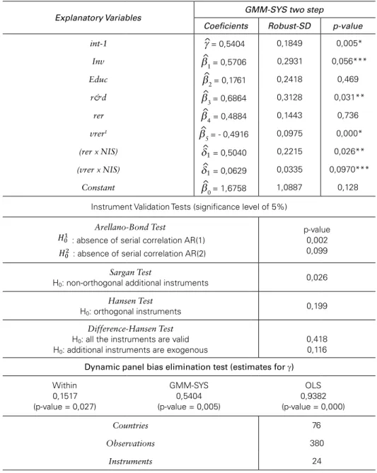
Tabela 2: Dynamic Model for Innovation with Dummies
Explanatory Variables
GMM-SYS two step
Coeficients Robust-SD p-value
int-1 ^g = 0,5404 0,1849 0,005*
Inv b^
1 = 0,5706 0,2931 0,056***
Educ b^2 = 0,1761 0,2418 0,469
r&d b^
3 = 0,6864 0,3128 0,031**
rer b^4 = 0,4884 0,1443 0,736
vrer1 b^
5 = - 0,4916 0,0975 0,000*
(rer x NIS) d^1 = 0,5040 0,2215 0,026**
(vrer x NIS) d^1 = 0,0629 0,0335 0,0970***
Constant b^0 = 1,6758 1,0887 0,128
Instrument Validation Tests (significance level of 5%)
Arellano-Bond Test !!!
: absence of serial correlation AR(1) !!! : absence of serial correlation AR(2)
p-value 0,002 0,099
Sargan Test
H0: non-orthogonal additional instruments
0,026
Hansen Test H0: orthogonal instruments
0,199
Difference-Hansen Test H0: all the instruments are valid H0: additional instruments are exogenous
0,418 0,116
Dynamic panel bias elimination test (estimates for g)
Within 0,1517 (p-value = 0,027)
GMM-SYS 0,5404 (p-value = 0,005)
OLS 0,9382 (p-value = 0,000)
Countries 76
Observations 380
Instruments 24
Source: Own elaboration based in the regressions.
Notes: 1. vrer = (vps5); * significant at 1%, ** significant at 5%, *** significant at 10%.
According to Table 2, yet again the parameter that captures the effect of the education variable is not significant and the coefficients of the variables int-1, r&D and investment were statistically significant to the levels of 1%, 5% and 10%, respectively, and have the expected signs.
devaluation (rEr) and exchange rate volatility (vrEr) over innovation differ between the two country groups (d^1 ≠ 0) and (
^
d2 ≠ 0). The effect of the devaluation
of the rEr over innovation has been shown to be significant only to the groups of countries with a mature NIs. The estimated coefficient for the rEr variable is not statistically significant (b^4 = 0), so that, for the countries with a well developed NIs, the coefficient that measures sensitivity to innovation relative to the devaluation of the real exchange rate (b^4 + d^1 ) is limited to
^
d1 = 0,5040, statistically significant to
5% and with the expected signal. This result indicates that for a 10% devaluation in the rEr over a period of three years, an increase of innovation of about 5% is to be expected over the same period.
with regard to the effect of volatility of rEr over innovation, the results show that this effect is lesser in countries with a mature NIs. For the countries with a mature NIs this effect is measured by (b^5 + d^2 ) and for the other countries by
^ b5 . It was expected that b^5 < 0 and d^2 > 0 indicating that an increase in the volatility of
the rEr would affect the countries with a mature NIs to a lesser degree, in a mag-nitude equal to the value of d^2. The results show that^b5 = -0,4916 (significant to
the level of 1%) and d^2 = 0,0629 (significant to the level of 10%). Thus, in the
countries with a mature NIs the effect of exchange rate volatility over innovation is lesser when compared to the other countries (-0,4916 + 0,0629 = – 0,4287).
In terms of elasticity, a 10% increase in exchange rate volatility reduces in-novation by 7,2% in countries with a developed NIs and by 8.2% in the other countries. Therefore, the hypothesis that in the presence of a developed (mature) NIs in a country the effects of exchange volatility are “smoothened” is confirmed.
cONclUsION
In this article we have presented an empirical contribution to explain the ex-change rate-innovation relationship. The hypotheses that both the devaluation and volatility of the real exchange rate affect technological innovation and that this effect differs between country groups with mature NIs (in which interactions and information flows among agents are greater and stronger) and those where the NIs does not exist or is underdeveloped (there are no interactions or they are very weak) were tested through a system GMM estimator using an empirical model based on the Evolutionary Theory.
significant only to the group of countries with mature NIs – where the information flow is greater. For the other countries, the devaluation does not seem to affect in-novation production.
In relation to the real exchange rate volatility, the results show it affects in-novation negatively in both country groups. however, for the countries with well developed NIs the effect is lesser when compared to the other countries (a 10% increase in volatility reduces innovation in around 7,2% for the NIs-developed group and in 8,2% in the other countries). This difference can be explained by the fact that in a mature innovation system the bonds between the “key-agents” to the innovation process are stronger and completely formed, besides there being a big-ger number of agents working in the interaction channels. Furthermore, the firms of the countries with mature NIs show greater robustness on financial aspects and market position. Thus, these factors can ease the harmful effects of exchange rate volatility over information flow, despite the exchange rate volatility affecting the uncertainty in the corporate environment and affecting the revenue of the firms.
rEFErENcEs
Aghion, Philippe; Bacchetta, Philippe; ranciere, romain; rogoff, Kenneth (2006).“Exchange rate
volatility and Productivity Growth: The role of Financial Development”. NBER Working Paper.
series, 12117. cambridge.
Albuquerque, Eduardo da Motta (1996). “sistema Nacional de Inovação no Brasil: uma análise
intro-dutória a partir de dados disponíveis sobre a ciência e a tecnologia”. Revista de Economia
Políti-ca, 16 (3): 56-72.
Albuquerque, Eduardo da Motta (2009). “catching up no século xxI: construção combinada de
sistemas de Inovação e de Bem-Estar social”. In: sicsú, João; Miranda, Pedro (Org). Crescimento
Econômico: Estratégias e Instituições. rio de Janeiro: IPEA. 55-84.
Araújo, Eliane (2009). “volatilidade cambial e crescimento Econômico em Economias em Desenvol-vimento e Emergentes”. In: II Encontro Internacional da Associação Brasileira Keynesiana. Porto Alegre.
Arellano, Manuel; Bond, stephen (1991). “some Tests of specification for Panel Data: Monte carlo Evidence and an Application to Employment Equations”. Oxford: Oxford University Press. Review of Economic Studies, 58(2): 277-297.
Arellano, Manuel; Bover, Olympia (1995). “Another look at the instrumental variable estimation of
error-components models”. Journal of Econometrics, Elsevier, 68(1): 29-51.
Atella, vincenzo; Atzeni, Gianfranco Enrico; Belvisi, Pier luigi (2003). “Investment and exchange rate
uncertainty”. Journal of Policy Modeling, (25): 811-824.
Bernardes, Américo Tristão; Albuquerque, Eduardo da Motta (2003). “cross-over, thresholds, and
in-teractions between science and technology: lessons for less-developed countries”. Research Policy,
32 (5): 865-885.
Bhaduri, A; Marglin, s (1990). “Unemployment and the real wage: the economic basis for contesting
political ideologies”. Cambridge Journal of Economics, 14 (4): 375-393.
Biesebroeck, J. v (2005). “Exporting raises productivity in sub-saharan African manufacturing firms”. Journal of International Economics, 67: 373-391.
Bittencourt, Mauricio vaz lobo; larson, Donald w.; Thompson, stanley r (2007). “Impactos da
vola-tilidade da Taxa de câmbio no comércio setorial do Mercosul”. Estudos Econômicos, 37 (4):
Blundell, richard; Bond, stephen (1998). “Initial conditions and moment restrictions in dynamic panel
data models”. Journal of Econometrics, Elsevier, 87 (1): 115-143.
Bond, stephen (2002). “Dynamic panel data models: A guide to micro data methods and practice”.
londres: cemmap, Institute for Fiscal studies. Working Paper cwP09/02. website:
http://cem-map.ifs.org.uk/wps/cwp0209.pdf. Acessado em: 20 setembro de 2013.
Bosworth, B.; collins, s.; chen, y (1996). “Accounting for Differences in Economic Growth, in struc-tural Adjustment and Economic reform: East Asia, latin America, and central and Eastern
Eu-rope”. Institute of Developing Economies, Tokyo.
Bresser-Pereira, luiz carlos; Nakano, yoshiaki (2003). “crescimento Econômico com Poupança
Exter-na?” Revista de Economia Política, 23 (2): 3-27.
Bresser-Pereira, luiz carlos (2015). “The Access to Demand”. Brazilian Keynesian Review, 1 (1): 35-43.
calderón, césar; Kubota, Megume (2009). “Does higher Openness cause More real Exchange rate
volatility?” The word Bank: Policy Research Working Paper 4896. Apr.
cameron, A. colin; Trivedi, Pravin. K (2005). “Microeconometrics: Methods and applications”. New
york: Cambridge University Press, caps. 21 e 22.
campos, Marlon Torres; resende, Marco Flávio da cunha (2009). “Taxa de câmbio real e
cresci-mento Econômico: Novos canais de transmissão”. In.: Encontro Nacional de Economia da
ANPEC, 37. Anais. Foz de Iguaçu.
carmo, Alex sander souza; Bittencourt, Maurício vaz lobo (2013). “O efeito da volatilidade da taxa real de câmbio sobre a diversificação da pauta de exportação do Brasil: uma investigação
empí-rica. In: Encontro Nacional de Economia da ANPEC, 41. Anais. Foz de Iguaçu.
clark, Peter et al. (2004). “Exchange rate volatility and Trade Flows: some New Evidence”. FMI,
washington.
curado, Marcelo; rocha Marcos; Damiani, Daniel (2011). “câmbio e crescimento Econômico: uma
comparação entre economias emergentes e desenvolvidas”. Revista de Economia Política, 31 (4):
528-550.
Dollar, David (1992). “Outward-oriented Developing Economies really do Grow More rapidly:
evi-dence from 95 lDcs, 1976-1985”. Economic Development and Cultural Change, chicago, 40
(3): 523-544.
Dosi, Giovanni; Freeman, christopher; Fabiani, silvia (1994). “The Process of Economic Development:
Introducing some stylized facts and theories on technologies, firms and institutions”. In.:
Indus-trial and Corporate Change, 3:1-45. Oxford University Press.
Eichengreen, Barry (2008). “The real exchange rate and economic growth”. commission on Growth
and Development. International Bank for Reconstruction and Development/World Bank. Work
Paper No 4. washington.
Freeman, christopher (1995). “The National system of Innovation in historical Perspective”.
Cam-bridge Journal of Economics, london, 19 (1): 5-24.
Freeman, christopher (2002). “continental, national and sub-national innovation systems -
comple-mentarity and economic growth”. Research Policy, 31 (2): 191–211.
Freeman, christopher; soete, luc (1982 [2008]). “A Economia da Inovação Industrial”. campinas: Editora Unicamp. caps. 10, 12, 13 e 15.
Gala, Paulo (2008). “real Exchange rate levels and Economic Development:theoretical analysis and
empirical evidence”. Cambridge Journal of Economics, cambridge, 32 (273-288).
Gala, P.; libanio, G. A (2008). “Exchange rate policies, patterns of specialization and economic
deve-lopment”. In: 10th International Post Keynesian Conference, Kansas city - EUA.
Greene, william h (2012). “Econometric Analysis”. 7th ed. New york: Prentice hall. caps. 08 e 11. herskovic, Bernard; ribeiro, costa leonardo; Albuquerque, Eduardo da Motta (2008). “Efeitos
recí-procos entre finanças e inovação”. Belo horizonte: UFMG/cEDEPlAr, Texto para discussão 332.
hooper, P.; Kohlhagen, s.w (1978). “The effect of exchange uncertainty on the prices and volume of
Kleinknecht, A.; van Monfort, K.; Brouwer, E. (2002). “The non-trivial choice between innovation
in-dicators”. Economics of innovation and new technology, 11 (2): 109-121.
lundvall, Bengt-Âke (1988). “Innovation as an Interactive Process: from user-producer interaction to
the national system of innovation”. In: DOsI, G. et al. Technical change and economic theory.
london: Pinter. cap 17.
lundvall, Bengt-Âke (1992). (Ed.) “National systems of Innovation: towards a theory of innovation and interactive learning”. london: Pinter. caps 01 e 03.
lundvall, Bengt-Âke et al. (2002) “National systems of Production, Innovation and competence
Buil-ding”. Research Policy, 31: 213–231.
Marques, David luís (2000). “Modelos Dinâmicos com Dados em Painel:revisão de literatura”.
Dis-sertação (Mestrado em Economia) - centro de Estudos Macroeconómicos e Previsão, Faculdade de Economia do Porto.
Missio, Fabricio José (2012). “câmbio e crescimento na Abordagem Estruturalista-Keynesiana”. Tese (Doutorado em Economia) - centro de Desenvolvimento e Planejamento regional, Universidade Federal de Minas Gerais, Belo horizonte.
Mukhtar, Tahir; Malik, saquib Jalil (2010). “Exchange rate volatility and Export Growth:Evidence
From selected south Asian countries”. Espoudai Journal of Economics and Business, 60 (3-4):
58-68.
Nelson, richard r.; winter, sidney G (1982 [2005]). “Uma Teoria Evolucionária da Mudança Econô-mica”. campinas: Editora da Unicamp. caps. 04, 05 e 11.
Nelson, richard r. (1996 [2006]). “As Fontes do crescimento Econômico”. campinas: Editora Uni-camp. caps. 02, 06, 07 e 09.
Perée, Eric; steinherr, Alfred (1989). “Exchange rate Uncertainty and Foreign Trade”. European
Eco-nomic Review. 33 (6): 1241-1264.
ribeiro, leonardo c.; ruiz, ricardo M.; Bernardes, Américo T.; Albuquerque, Eduardo M. (2006)
“science in the developing world: running twice as fast?” Computing in Science and Engineering,
8: 81-87.
rodrik, Dani (2007). “The real exchange rate and economic growth: comments and Discussion”.
Pro-ject MUsE – Today’s research, Tomorrow’s Inspiration. Brookings Papers on Economic Activity,
p. 365-412.
romero, João Prates (2011). “Desenvolvimento Econômico e Mudança Estrutural: Teoria e evidência a partir de um enfoque multisetorial”. Dissertação (Mestrado em Economia) - centro de Desen-volvimento e Planejamento regional, Universidade Federal de Minas Gerais, Belo horizonte.
roodman, David (2009). “how to do xtabond2:An introduction to difference and system GMM in
stata”. The Stata Journal, 09 (1): 86-136. college station, Texas.
schnabl, Gunther (2007). “Exchange rate volatility and Growth in small Open Economies at the Emu
Periphery”. Frankfurt: European central Bank. Working Paper series n. 773.
smith, Keith (2005). “Measuring Innovation”. In: Fagerberg, Jan; Mowery, David; Nelson, richard r.
The Oxford Handbook of Innovation. Oxford: Oxford University. cap. 06.
williamson, John (2003). “Exchange rate policy and development”. In: Initiative for Policy Dialogue
Task Force on Macroeconomics, columbia, New york.
woo, wing Thye (2004). “some fundamental inadequacies of the washington consensus:
Misunders-tanding the poor by the brightest”. Earth Institute, columbia University.
ANNEx 1: sPEcIFIcATION TEsTs FOr ThE DyNAMIc INNOvATION MODEl
CHOW: H0: Restricted model (Pooled) H1: Unrestricted model (fixed effects)
F (70, 163) = 3.48 Prob > F = 0.0000 Rejects H0: Panel data model is more appropriate.
BREUSCH-PAGAN (LM TEST): H0: Pooled Model
HA: Random Effect Model
Chibar2(01) = 3.77 Prob > chibar2 = 0.0261 Rejects H0: Panel data model is more appropriate.
HAUSMAN TEST:
H0: There is no correlation between ai and the regressors Xit’s – both models are consistent, but the fixed effects model is less efficient
HA: There is correlation – both are consistent, but fixed effects one is more efficient
Chi2(6) = 140.74 Prob > chi2 = 0.0000 Rejects H0: Dynamic model of EF for innovation is more efficient
Fonte: Own elaboration based in the regressions from stata 12.0.
ANNEx 2: rEsUlT OF ThE EsTIMATE OF ThE DyNAMIc FIxED EFFEcTs MODEl FOr INNOvATION wIThOUT DUMMIEs UsING vPs3, vDP5 AND vDP3
As A MEAsUrE FOr rEAl ExchANGE rATE vOlATIlITy
Explicative
GMM-SYS two step GMM-SYS two step GMM-SYS two step
(VPS3) (VDP5) (VDP3)
b Robust
SD p-value b
Robust
SD p-value b
SD
Robust p-value
int-1 0,4620 0,2223 0,041** 0,4409 0,2295 0,059*** 0,4978 0,2703 0,070***
inv 0,3097 0,3264 0,346 0,2514 0,2436 0,063*** 0,2654 0,2589 0,309
educ 0,5748 0,3498 0,105 0,4818 0,3583 0,183 0,3432 0,4255 0,423
p&d 0,8820 0,4335 0,046*** 0,9413 0,4092 0,024** 0,8738 0,4828 0,075***
dcr 0,3878 0,2099 0,069*** 0,4657 0,2293 0,046** 0,2977 0,1645 0,075***
vcr -0,6227 0,2802 0,029** -3,4855 1,5210 0,025** -0,3895 0,2116 0,070***
Instrument Validity Tests (Significance Level of 5%)
Arellano-Bond
!!! : Serial non-correlation
AR(1) !!!: Serial non-correlation
AR(2)
p-value p-value p-value
0,002
0,095
0,019
0,486
0,010
Sargan H0: non-orthogonal additional instruments
0,015 0,001 0,001
Hansen H0: Orthogonal
ins-truments
0,061 0,063 0,057
Difference-Hansen H0: All valid instruments H0: Additional
exogenous instruments
0,089
0,087
0,109
0,072
0,065
0,277
Countries Observations
Instruments
76 380
22
Fonte: Own elaboration based in the regressions.