Effects of overvaluation and exchange rate
volatility over industrial investment: empirical
evidence and economic policy proposals for Brazil
JOSÉ LUIS OREIRO FLAVIO A. C. BASILIO
GUSTAVO J. G. SOUZA*
The present article aims to analyze the recent behavior of real exchange rate in Brazil and its effects over investment per worker in Brazilian manufacturing and extractive industry. Preliminary estimates presented in the article shows an over-val-uation of 48% of real exchange rate in Brazil. The reaction between the level (and volatility) of real exchange rate and investment (per worker) in Brazil is analyzed by means of a panel data econometric model for 30 sectors of Brazilian manufactur-ing and extractive industry. The empirical results show that the level and volatility of real exchange rate has a strong effect over investment per worker in Brazilian industry. Finally, we conclude the article presenting a proposal for a new macroeco-nomic regime that aims to produce an acceleration of ecomacroeco-nomic growth of Brazilian economy and, by that, a catching-up process with developed countries.
Keywords: real exchange rate; economic development; structuralist development macroeconomics.
JEL Classiication: L5; O11; F41.
INTRODUCTION
The general issue formulated for the tenth edition of the Economic Forum of São Paulo concern the strategy required for Brazil double its per capita income in
*Respectively, Professor at Instituto de Economia da Universidade Federal do Rio de Janeiro, Level IB Researcher at CNPq and President of Brazilian Keynesian Association. E-mail: [email protected]; PhD in Economics at Universidade de Brasília (UnB). E-mail: [email protected]; PhD in Economics at Universidade de Brasília (UnB) and professor at Universidade Católica de Brasíla (UCB). E-mail: [email protected]. Submitted: 4/October/2013; Approved: 10/January/2014.
15 years. Based on the known “rule of 70”, for a country to double its per capita income in 15 years, the rate of growth required for its per capita income double in this period shall equal the 70/15, i.e., 4.66% p.a.. Considering that the Brazilian population is currently growing around 0.6% p.a. for Brazil to double its per capita income in 15 years, GDP would have to grow at rate of 5.26% p.a. during this period. Given that in the last 20 years (1992-2012) the average growth of the Brazilian economy was 2.96% p.a., according IPEADATA, to double Brazil’s per capita income, in such a short space of time, would be necessary to increase the rate of GDP growth by almost 100%.
Given that rate unemployment is slightly below 6%, a number considered by some economists to be close to a situation of full employment, an acceleration of this magnitude in real GDP growth rate will only be possible through a significant increase in labor productivity, which requires a significant increase in investment and capital accumulation.
Based on Harrod-Domar growth model, and assuming a capital-output ratio equal to 3 and a rate of depreciation of fixed capital equal to 3.5% p.a., the rate of investment required to double per capita income in 15 years is 26.28% of GDP. An investment rate as a proportion of GDP close to 18%, as observed in recent years, is clearly insufficient to produce an acceleration of this magnitude in real GDP growth rate.
What are the policies that can be adopted to induce a stronger pace of capital accumulation and, therefore, a faster growth of real GDP? In particular, what is the appropriate exchange rate policy for Brazil will be able to double its per capita income in 15 years?
This question is a complete non-sense for liberal economists. For them the rel-evant variable to explain the growth of per capita income is the Total Factor Pro-ductivity (cf. Veloso, Ferreira & Person, 2013). In this context, the Brazilian econ-omy is semi-stagnant due to factors like high taxes (cf. Ellery & Teixeira, 2013), low rate of government saving (see Bacha & Bonelli, 2013) or low investment in education (cf. Ferreira & Veloso, 2013). The restrictions on growth of the Brazilian economy came, therefore, from the supply side of the economy, so that changes in exchange rate policy will have little or no effect on growth perspectives of Brazil.
characterizes a growth regime of export-led type. In this context, the occurrence of catching-up requires that the ratio of these elasticities are greater than one; which requires, in turn, a diversified production structure and firms that are operating fairly close to the technological frontier.
Until recently, the literature of demand-led growth downplayed the existence of a relationship between the income elasticities of imports and exports and the level of real exchange rate. However, economists of the so-called Structuralist Development Macroeconomics has argued for the existence of a relationship between the level of the real exchange rate and the income elasticities of the Thirlwall model. More specifically, it is argued that deviations of real exchange rate with respect to industrial equilibrium level (Bresser-Pereira, Oreiro & Mar-coni, 2013) result in a reduction in the rate of capital accumulation which leads to perverse changes in the productive structure of a country and therefore in in-come elasticity of exports and imports, which give rise to a reduction in the growth rate compatible with the balance of payments equilibrium, and therefore can derail the catching-up process.
This article aims to analyze the recent behavior of the real exchange rate in Brazil, emphasizing its state of chronic overvaluation even after recent devaluations of nominal exchange rate. Preliminary estimates presented in this paper point to an overvaluation of about 48% of the real exchange rate in Brazil. The relationship between the level (and volatility) of the real exchange rate and investment (per worker) in Brazil is analyzed using an econometric model with panel data for 30 sectors of manufacturing and extractive industry. The empirical results support the hypothesis that the real exchange rate is a key variable in determining the capital accumulation and long-run growth path. Finally, we conclude this paper by present-ing a proposal for a macroeconomic policy framework to enable faster growth of the Brazilian economy and therefore the process of catching-up with respect to developed countries.
THE RECENT BEHAVIOR OF THE ExCHANGE RATE IN BRAzIL: TOWARDS THE INDUSTRIAL EqUILIBRIUM?
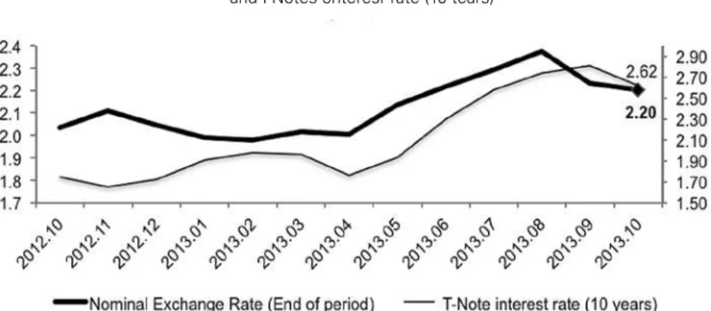
Source: IPEADATA. Prepared by the authors. The values measured on the left vertical axis refers to the nominal exchange rate, while the values measured on the right vertical axis refers to the interest rate of the 10 years T-Notes.
Although the nominal exchange rate has returned to appreciate, standing at around R$ 2.20-2.30; it is unlikely that it will return to the levels prevailing in early 2013. In this context, we should ask what are the likely effects of the devalu-ation of the nominal exchange rate on the Brazilian economy. In particular, does the current level of exchange rate will allow the recovery of the Brazilian economy’s competitiveness to be closer to the so-called industrial equilibrium, leveraging a greater dynamism of the industrial sector and, therefore, a more robust pace of economic growth1?
To analyze the impact of the depreciation of the nominal exchange rate on the competitiveness of Brazilian industry we need to look at the effect on the real ef-fective exchange rate for exports of manufactured products2. This time series can be viewed in Figure 2. As we can see in Figure 2, the real effective exchange rate clear shows a trend to appreciation in the period from January 2003 to June 2008. Due to the impact of the international financial crisis, detonated from the bank-ruptcy of Lehman Brothers in September 2008, the real effective exchange rate has suffered a rapid depreciation which, however, is reversed at the beginning of 2009. Ended the effects of the international financial crisis on the Brazilian economy observed a tendency towards stability of the real effective exchange rate until
Au-1 Regarding the relationship between the exchange rate overvaluation, loss of competitiveness and
semi-stagnation of the Brazilian economy, see Oreiro (2013).
2 This series is calculated by IPEA and is a measure of the competitiveness of Brazilian exports calculated
by the weighted-average index of the purchasing power parity of 16 major trading partners of Brazil. The purchasing power parity is defined as the quotient between the nominal exchange rate (R$/unit of foreign currency) and the relationship between the Wholesale Price Index (WPI) of the country concerned and the National Consumer Price Index (INPC/IBGE) from Brazil. The weights used are the contributions of each partner of Brazilian exports of manufactured goods in 2001.
gust 2011, when it begins a process of depreciation, reaching in August 2013 a plateau near the prevailing in mid-2005.
Source: IPEADATA. Prepared by the authors.
The return of the real effective exchange rate to the levels prevailing in mid-2005 means that the Brazilian manufacturing industry will retrieve its dynamism? At first glance the answer would be yes, since in the period in which the real effective ex-change rate was more depreciated, the manufacturing industry was more dynamic. In fact, between January 2003 and August 2008, according to data from IPEADATA reproduced in Figure 3, the physical production of manufacturing industry grew up 28.71%; whereas in the period between March 2010 and August 2013 the physical production of manufacturing industry was virtually stagnant, showing a slight drop of 2.75%.
Source: IPEADATA. Prepared by the authors.
A more careful analysis, however, leads us to be more pessimistic about the impact of the recent depreciation of the nominal exchange rate on the prospects of expansion of the production in manufacturing industry. As we can see in Figure 3,
Figure 2: Real Effective Exchange Rate – Manufactures Exports
the depreciation of the real effective exchange rate, which occurred from January 2012, had no noticeable effect on the trend of the physical production in manufac-turing industry, which continues to oscillate around a stationary level. This means that the depreciation of the real exchange rate that has occurred so far has not been large enough to recover the competitiveness of Brazilian industry.
This observation becomes clearer when we look at the behavior of the relation-ship between real effective exchange rate/wages3, shown in Figure 4, which is an indicator of the profitability of exports from the manufacturing industry.
Source: IPEADATA. Prepared by the authors.
As we can see in Figure 4, between January 2003 and December 2013 the real effective exchange rate deflated by nominal wage presented an appreciation of incredible 66.78%. This means, first of all, that the recent depreciation of the nominal exchange rate has had no noticeable effect on the relationship under con-sideration, thereby indicating that the competitiveness of the manufacturing indus-try remains unchanged. Secondly, but no less important, the loss of competitiveness of the manufacturing industry, not only the trend towards appreciation of the ex-change rate recorded since 2003, but also the wage growth at a pace above labor productivity growth that occurred in this period.
What should be the real effective rate exchange rate to reestablish the competi-tiveness of Brazilian manufacturing industry? To answer that question, let us as-sume that the ratio between real effective exchange rate/wage prevailing in mid-2005 is appropriate to restore the competitiveness of industry, since, between 2004 and 2007, the physical production of manufacturing industry expanded at rates more robust. In May 2005, the relationship real effective exchange rate/wage was equal to 101.99. In June 2013, the real effective exchange rate and the ratio real
3 Index calculated from the average wages nominal (FIESP), real exchange rate (R$) / US dollar (US$)
— monthly average — sale (Central Bank of Brazil), Exchange rates for 16 selected countries / US dollar (US$) — monthly average (IMF) and the weighting of 16 selected countries of Brazilian exports (Secex).
effective exchange rate/wage were, respectively, 97.26 and 52.91. Thus, for a simple proportional rule, the real effective exchange rate compatible with the value of the ratio real effective exchange rate/ wage prevailing in May 2005 should be of 187.47, an overvaluation of 48.12%!
This simple exercise points to the fact that the recent depreciation of the nomi-nal exchange rate is much lower than that required to restore the competitiveness of the manufacturing industry, a sine qua non condition for obtaining more robust growth rates for real GDP. It follows that while the government does not operate a profound change in macroeconomic matrix, which allows obtaining a more com-petitive exchange rate in the same time that keeping inflation in low and stable levels, the Brazilian economy will be doomed to get mediocre growth rates. We will return to this issue.
INTERNATIONAL EVIDENCE ON THE VOLATILITy OF THE ExCHANGE RATE AND ITS EFFECT ON INVESTMENT (1995-2013)
The hypothesis that not only the level of the real exchange rate, but also the volatil-ity of the nominal exchange rate affects investment decisions was empirically sup-ported by Darby et al. (1999). Thus, there would be two related channels acting on agent’s investment decisions. The first, the traditional, which relates the real exchange rate to external competitiveness and economic activity: “The exchange rate is one of most important macroeconomic variables in the emerging and transition countries. It affects inflation, exports, imports and economic activity” (Edwards, 2006, p. 28). The second effect, relates the nominal exchange rate volatility to investment. Is was argued that the flow of new information on the market, in an environment of uncertainty, asymmetric information and incomplete markets, can both reduce the volatility but also increase it. This means that the relationship between volatility and increased un-certainty is not linear. This statement also does not mean that the elimination of ex-change rate volatility automatically eliminates the uncertainty and therefore stimulates investment but yes, from certain level of volatility, uncertainty is so large that the agents simply choose to postpone their investment decisions. Thus, the effect of volatility on the economy, in particular on industry, should not be homogeneous, being more sig-nificant for those with less monopoly power and lower technological intensity, i.e., for those industries more susceptible to price fluctuations.
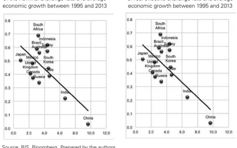
Considering the data of the nominal bilateral exchange rate with the US dollar of the countries of G204, in the period from 01.02.1995 to 09.10.2013, totalling 4,877 observations, and the monthly real effective exchange rate calculated by BIS
4 Argentina was excluded from the analysis due to lack of credibility of the exchange rate data. As we
(Bank for International Settlements), from December 1994 to July 2013, with 224 observations, we proceed with the analysis between the relationship of exchange rate variation with average economic growth.
The results are consistent with the empirical evidence cited by literature, so that exchange rate volatility is negatively correlated with economic growth, according to Figures 5 and 6.
Figure 5: Relationship between daily variation of the nominal exchange rate and average economic growth between 1995 and 2013
Figure 6: Relationship between montly variation of real effective exchange rate and average economic growth between 1995 and 2013
Source: BIS, Bloomberg. Prepared by the authors.
Table 1: Correlation between variations of exchange rates (nominal and real) and average growth of countries between 1995 and 2013
Country
Average Growth Rate
Mean Std. Deviation
non-parametri
c VaR (95%)
non-parametri
c VaR (99%)
Mean Std. Deviation
non-parametri
c VaR (95%)
non-parametri
c VaR (99%) South Africa 3,2 0,69 0,77 2,12 3,38 2,44 2,41 6,56 14,79 Australia 3,3 0,56 0,58 1,58 2,61 1,80 1,56 4,25 6,09 Brazil 3,0 0,59 0,80 2,02 3,76 2,54 3,14 7,63 21,81 Canada 2,5 0,37 0,37 1,10 1,81 1,15 1,04 2,66 5,44 Chile 4,6 0,39 0,42 1,16 1,90 1,50 1,34 4,04 6,23 China 9,7 0,03 0,06 0,15 0,27 1,18 0,91 2,87 4,22 South Korea 4,5 0,45 0,85 1,36 3,58 1,73 3,01 5,81 13,38 India 6,7 0,22 0,32 0,81 1,51 1,24 1,06 3,48 5,20 Indonesia 4,4 0,62 1,43 2,39 6,15 3,10 6,48 13,11 31,04 Japan 0,9 0,50 0,49 1,37 2,33 1,96 1,70 5,45 8,54 Mexico 2,5 0,48 0,68 1,40 3,06 2,07 3,20 5,42 14,42 United Kingdom 2,2 0,41 0,37 1,12 1,71 1,09 1,03 3,00 5,72 Turkey 4,4 0,57 0,95 1,73 3,66 2,39 2,61 9,36 12,62 Russia 3,3 0,34 1,11 1,09 2,65 2,01 4,06 5,47 15,32 -0,68 -0,30 -0,53 -0,34 -0,27 -0,15 -0,12 -0,19 Daily Nominal Exchange Rate Montly Real Exchange Rate
Correlation
For calculating the volatility, in addition to the usual statistics measures, we used the VaR (Value at Risk) approach, derived from the probability distribution of asset,
f (w). The choice of this measure stems from the international banking regulations established by Basel and followed by major central banks in the world. The risk associated of fluctuation of the exchange rate is part of the menu of concerns of regulatory requirements, so that the higher the risk exposure, the greater the capital requirements by banks and thus lower the capacity of lending and leverage.
In this context, given the level of confidence, c, it is estimated the worst possible realization, W*, such that the probability of exceeding this value of trust is given by:
c
f w dw
w
=
∗∞
∫
( )
Alternatively, the probability that a value smaller than w*occurs, with p P w W= ( ≤ ∗),is :
c
wf w dw
− =
∗−∞
∫
( )
1
==
P w W
(
≤
∗)
=
p
Assuming the data of daily variations (for nominal exchange rate) and monthly variations (for the real effective exchange rate) are independent and identically dis-tributed, the VaR indicates at the level of confidence 95% and 99%, the largest daily or monthly expected loss, as the case. Tables 1, 2 and 3 and Figure 7 (at the end of this article, on pp.369) summarize the results of calculation for both, para-metric and non-parapara-metric approach.
From the data presented in Tables 2 and 3 (see electronic edition), it is noted that the relative VaR exposure to foreign exchange rate in Brazil is quite high, which means high intensity in the exchange rate volatility and therefore high probability of maximum expected loss in portfolio of agents, particularly banks. However, the Brazilian data are in line with the values obtained by the major emerging countries of the G20, with the exception of Indonesia, whose daily VaR reached the amazing mark 26.99% (parametric) and 37.65% (non-parametric).
DETERMINANTS OF INVESTMENT IN BRAzILIAN INDUSTRy (1996-2007)
Taking as starting point the econometric model of Darby et al. (1999), we esti-mate the determinants of investment in Brazilian extraction and manufacturing industry taking into consideration not only the traditional purposes of capital cost and mark-up, but also on positive elements related to business opportunities, and negative related to uncertainties of investment decisions.
Given that investment per worker is the relevant variable in terms of output growth in the long run, we develop an econometric analysis based on six models with panel data for 30 industrial sectors of the Brazilian national accounts system (SCN-econometric analysis 42) in the period between 1996 and 2007. In this sense,
the estimation method chosen allows different analysis of those proposals in Darby et al. (1999) model, because our model takes into consideration the sectorial het-erogeneities, as suggested by the authors in the original model. Furthermore, the analysis developed not only checks the effects of real exchange rate on investment per worker, but also the effects of exchange rate volatility (uncertainty effect) causes in investment decisions. Additionally, we analyze the effects of investment oppor-tunities through the traditional channel of Tobin’s q5 and also about the mark-up effects on investment decisions. As a proxy of the latter variable, we use the relative price of industrial sector i on the economy general price level. As a robustness test, we have replaced the relative price for traditional variables such as the unit labor cost and labor productivity. Furthermore, we tested the effects of Harrodian ac-celerator on investment decisions. Finally, we replaced the volatility of the real exchange rate by the volatility of nominal exchange in order to verify the robust-ness of the empirical results.
1. Description of model variables and main results
Investment per worker: calculated at constant prices of 1995, from the system of national accounts of IBGE.
Real Effective Exchange rate REER: The real exchange rate (or effective rate) is the nominal rate deflated by a similarly weighted average of foreign price or cost. In particularly, the calculation of the real effective exchange rate is made from BIS data. To this end, we consider a basket of currencies consisting of 61 countries, so that the nominal exchange rate is weighted by the bilateral price on trading part-ners. In addition, the weighting system, itself, is based on Turner and Van ’t dack (1993) and takes into account the manufacturing transactions flows between coun-tries. Algebraically, the methodology is expressed by:
Weight of imports: w m m i m j i j =
Weight of exports: w w x y y x i x j i j i i h i h = + ∑ + + ≠
∑k i ∑
j k j i k k h k h x x x y x
Average weight: wi=
mjj j j i m j j j i x
x m w
x
x m w
+ + +
Where: j i
j
x m( ii
is the export of the economy for the e
) j cconomy
x m is the total export of the ecj j
i
( ) oonomy
y is the total domestic supply of mi j
a
anufatured goods in the economy x is th
i h
i
∑
hhe export of h(excluding j)foriHowever, the BIS methodology calculated the real exchange rate is in terms of the currency of the country of origin. This means that the interpretation of the exchange rate is how much foreign currency can be purchased with a unit of the domestic currency. In other words, “with a one real buy how many dollars is pos-sible to buy”.
To invert the logic, we proceed with the following algebraic calculus:
real exchange rate – notation Brazil = 1/(1+ exchange rate variation – BIS notation
Real Effective Exchange Rate Volatility: calculated on the basis of the monthly volatility of the real effective exchange rate.
Tobin Q: calculated from the ratio of the market value of companies listed on BMF Bovespa for its respective book value. The aggregate index is calculated from the weighting of individual values by asset of the company.
Cost of Capital: Brazilian average annual long-term interest rate (TJLP). Relative price: industrial mark-up proxy, calculated from the ratio of the sectoral price index by the General index of the economy, both calculated from the SCN (system of national accounts) of the IBGE.
Unit labor cost: using the labor productivity data and wages per worker at constant prices of 1995, it is estimated the unit cost of labor by each industrial sector.
Gross value added: obtained from the SNA, and supply and uses tables, calcu-lated at constant price of 1995.
Relative Labor Productivity: ratio between the average labor productivity of labor in industrial sector i by average labor productivity of the total economy.
Nominal Exchange Rate Volatility: calculated from daily data of nominal ex-change rate real/dollar aggregated on an annual basis.
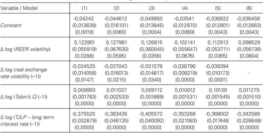
Table 4: Empirical results
Dependent variable: ∆ log (investiment per worker)
Variable / Model (1) (2) (3) (4) (5) (6)
Constant -0,04242 (0,013639) [0,0019] -0,044612 (0,016101) [0,0060] -0,049950 (0,013845) [0,0004] -0,03541 (0,012970) [0,0069] -0,036822 (0,012801) [0,0043] -0,036458 (0,012663) [0,0043]
∆ log (REER volatility)
0,122901 (0,055918) [0,0288] 0,127981 (0,067630) [0,0595] 0,126815 (0,060045) [0,0356] 0,102141 (0,055647) [0,0676] 0,112913 (0,053711) [0,0365] 0,098529 (0,056136) [0,0804]
∆ log (real exchange rate volatility (–1))
-0,034525 (0,014058) [0,0147] -0,037043 (0,016013) [0,0215] -0,031579 (0,014817) [0,0340] -0,036790 (0,008219) [0,0000] -0,039394 (0,010173) [0,0001]
-∆ log (Tobin’s Q (–1))
0,009993 (0,001783) [0,0000} 0,011037 (0,002533) [0,0000] 0,009112 (0,001669) [0,0000] 0,010012 (0,001531) [0,0000] 0,10139 (0,001545) [0,0000] 0,011270 (0,001510) [0,0000]
∆ log (TJLP – long term interest rate (–1))
∆ log (relative price (–1)) 0,171480 (0,072408) [0,0186] -0,167191 (0,074742) [0,0261] - -0,183334 (0,069713) [0,0090]
∆ log (unit labor cost (–1))
--0,246907 (0,119453) [0,0397]
- - -
-∆ log (gross value added ) -
-0,308105 (0,253269)
[0,2249]
- -
-∆ log (labor productivity (–1)) - -
-0,323720 (0,200390)
[0,1074]
-
∆ log (labor rel.
productivity (–1)) - - -
-0,306238 (0,205652)
[0,1376]
∆ log (NER volatitlity (–1)) - - - -
--0,039362 (0,008607)
[0,0000]
Observations: Cross-sections included: 30. Periods included: 10 years - 1998-2007. Total panel (balanced) observations: 300
Redundant fixed effects (likelihood ratio) 0,326785 gl. (29,265) 0,313718 gl. (29,265) 0,200379 gl. (29,264) 0,266450 gl. (29,265) 0,268253 gl. (29,265) 0,330388 gl. (29,265)
Normality test: Jarque-Bera 1,453363 [0,483511] 1,818856 [0,402755] 1,706006 [0,426133] 1,404904 [0,495369] 1,353664 0,508224 1,397585 0,497185
Method Panel EGLS (cross-section weights). Linear estimation after one-step weighting matrix. White cross-section standard errors & covariance (d.f. corrected).
Weighted Statistics
R2 0,163952 0,169393 0,158093 0,169274 0,168097 0,172352
Adjusted – R2 0,056686 0,062825 0,046477 0,062690 0,061363 0,066164
F — Statistic 1,528456
[0,035894] 1,589524 [0,024419] 1,416395 [0,067923] 1,588175 [0,024631] 1,574909 [0,026811] 1,623075 [0,019648] Unweighted Statistics
R2 0,101540 0,106688 0,113629 0,083488 0,084023 0,100710
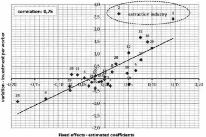
Figure 8: Relationship between investment per worker and fixed effects coefficient of econometric6 model (baseline model)
Figure 9: Relationship between investment per worker and fixed effects coefficient of econometric model (average of models) 7
6 In the graph above, we compare the percentage change in the period of 1996-2007 of the real value of
the investment, calculated from the System of National Accounts IBGE, with the estimated coefficients for each cross-section unit of the econometric model (M1) — benchmark. In this sense, considering that the higher the coefficient (constant) model, higher is the investment per worker, it is suggested that the estimates calculated for each sector are consistent with empirical evidence. Particularly, the greatest divergence occurs with the extractive industry. When we compare the estimated value with the actual real value reported, we found greater investment per worker than the result expected by the model. However, when considering that the extractive industry sector are companies such as Vale do Rio Doce and Petrobras, is justified by higher variation in investment per worker than predicted by the econometric model. 7 For the analysis, the averages were calculated from estimated coefficients in econometric models M2
2. Empirical analysis
From the econometric models (1) to (6) shown in Table 4, it is evident that the level of the exchange rate affects investment per worker, so that the exchange rate depreciation has positive effects on industrial investment decisions. In this sense, the result obtained corroborates the thesis of structuralist development macroeco-nomics that more depreciated exchange rate levels stimulate investment decisions by industrial sector.
The exchange rate volatility, by involving important elements related to uncer-tainty about the future behavior of the exchange rate, was highly significant in all estimated models. In addition, the exchange rate volatility appears to affect invest-ment decisions in a higher intensity than related to the level of the exchange rate. Apparently, the stability of the exchange rate by reducing the levels of volatility and
uncertainty has beneficial effects on investment decisions, which provides support to a regime of exchange rate administration.
The cost of capital, measured by TJLP, was highly significant, corroborating the need for industrial policies for the long-term investment and pointing to the need to reduce the value of the real interest rate in Brazil as a way to stimulate invest decisions and long-run economic growth.
Investment opportunities, estimated from Tobin’s q, were highly significant in all analyzes. This result brings an important component of the Keynesian theory of investment and signals the importance of using, in the future, this indicator for predicting the behavior of investment, since it is a leading indicator, prior lagged to investment decision itself.
The industrial mark-up was an important industrial component of investment decisions and highly significant in all tests developed.
To test the robustness of the model through the replacement of the mark-up by the unit cost of labor and later by relative productivity, high stability of the esti-mated coefficients for the other explanatory variables, corroborating the impor-tance of the result found in relation to the Exchange and its volatility.
technological intensity, is more sensitive to exchange rate effects than low techno-logical intensity, such as sector 29 (Other food products and beverages) or even the sector 12 (Sawmills and manufacture of woods products and furniture).
However, notably the industrial sectors linked to the extraction of commodities (Cme) showed strong dynamism related to investment, since in this sector include two of the largest Brazilian companies, namely: Petrobras and Vale do Rio Doce.
THE MANAGEMENT OF REAL ExCHANGE RATE
Neo-liberal economists argue that management of real exchange rate is impos-sible because the only thing that the monetary authority can do is determine the nominal exchange rate, not the real rate. This is because the variations of the nominal exchange rate generate exactly proportional variations in domestic price level in the long-term, thus leaving the real exchange rate outside the scope of action of the monetary authority. Moreover, it is also argued that the administration of the nominal exchange rate would only be possible in a context of financial openness to the outside, if the Central Bank failed to conduct monetary policy in order to meet domestic objectives (e.g., control inflation and/or stabilization of the level of output and employment). As democratic societies seem to demand the adoption of counter-cyclical policies by their respective Governments, in order to mitigate the effects of business cycles on the level of employment and welfare; it follows that the fixed exchange rate regime or managed regime is politically impracticable, and it should be, therefore, adopt floating exchange regime.
It is not true that the Central Bank can’t manage the real exchange rate with the instruments it has at its disposal, so it also is not true that the adoption of a system of fixed or managed exchange rates requires abandoning autonomous monetary policy, i.e., a policy geared to meet domestic objectives. In an economy in which the goods produced domestically are imperfect substitutes of goods produced abroad and where domestic assets are equally imperfect substitutes of assets denominated in foreign currency; not only the real exchange rate is a vari-able that, under certain conditions, can be administered by the Monetary Author-ity, as even this administration is done without loss of autonomy in the conduct of monetary policy.
To demonstrate the validity of this assertion let us consider a small open econ-omy that operates with a fixed exchange rate regime or with a managed regime8. Let S to be the nominal exchange rate, settled by the monetary authority, Ap(.) Is the absorption of domestic private sector, Y is domestic income,
ø
(.) the fraction of domestic absorption that is intended for the purchase of domestic goods G is the expense of government in real terms, X(.) is the quantity of domestic goods demanded by non-residents, r is the real rate of interest, T is a proxy of taxtions by the Government, Y* is the international income and P * is the interna-tional price level. The condition of equilibrium in the market goods is given by:
Y SP
P A Y T r G X
SP
P Y
p =
[
−]
+ + φ * , *; * (1)
We will assume that: (i) the economy operates at full-capacity, i.e., with a level of output equal to potential output, Yp; (ii) behavioral functions presented in (1) are homogeneous of degree one with respect to the capital stock, so that variations in the stock of aggregate capital does not alter the values of the endog-enous variables.
That said, the equilibrium condition in the goods market is given by:
Y SP
P A Y T r G X
SP
P Y
p= p p
− + +
φ * , *; * (2)
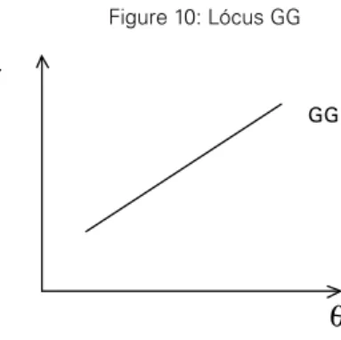
In equation (2) the endogenous variables are: G, T, S, y* e P*. By setting the real exchange rate as θθ =SP
P
*, equation (2) will define the locus of combinations
between real interest rate and real exchange rate for which the goods market is in equilibrium. Making the usual assumptions about the values of the partial derivatives with respect to behavioral functions r and q, we obtain the curve GG presented in Figure 10:
Figure 10: Lócus GG
r
GG
θ
Domestic residents may allocate their financial wealth, Wp, between money (M), domestic government securities (B), and foreign government bonds (B*). We sup-pose that domestic and foreign bonds are imperfect substitutes9 for each other so that, in equilibrium, their rates of return may be different. No-residents can also buy domestic bonds, such that the economy has a financially open account. The monetary authority may or may not impose restrictions on the purchase of
tic securities by foreigners or the purchase of foreign securities by domestic resi-dents. If these controls are imposed, the demand for domestic bonds by non-resi-dents will be a fraction l demand with absence of such restrictions10.
Let R to be the nominal domestic interest rate, R* the nominal international interest rate, b(.) the fraction of non-monetary wealth that domestic residents al-locate for the purchase of domestic bonds, b*(.) the fraction of wealth measured in foreign currency that non-residents allocate for buying international bonds, L(.) the actual demand for domestic money balances, L*(.) the real money demand for non-residents e WF the financial wealth of non-residents measured in the currency of their own country. We have then that the demand for residents and non-residents for domestic bonds is given by:
Bd R R W PL R Y W P
p p F
=b
(
− *)
−(
,)
+λSb* R – R*(
)
− *LL*(
R Y, *)
(3)
Assuming that the stock of domestic bonds is given by B and the central bank retains Bc of these securities in portfolio, the equilibrium in the domestic bond market is given by:
B B− c=b
(
R R− *)
Wp−PL R Y(
, p)
+λSb* R – R*(
)
WF−P LP* *(
R Y, *)
(4)
The aggregate financial wealth of the country is given by the sum between the wealth of the private sector, Wp, the wealth of the government, WG , and the wealth of the Central Bank, WC. In this way, we have that:
Wp+WG+Wc=
(
M+Bp+SFp*)
−B+(
SFc*+Bc−M)
=S F((
c*+Fp*)
−BF(5)
Where: Bp represents the domestic bonds owned by the private sector, c =S Fc +
* *
((
repre-)
sents the value in foreign currency of international bonds owned by the Central Bank (international reserves), =
(
*+Fp* is the foreign currency value of international se-)
curities owned by private domestic sector, M is the monetary base and BF represents value in terms of domestic currency owned by non-residents.From equation (5) we can see that the aggregate wealth is equal to financial claims against the rest of the world, except the financial rights of the rest of the world against domestic economy. We will call this resulting as net foreign assets, IIP. This value refers to the net investment position of the domestic economy measured in terms of their own currency. The net foreign assets measured in foreign currency is: IIP IIP
S *= .
Assuming thatWc = 0 and taking into account thatWG = – B, we have that S IIP* = Wp – B, i.e.:
Wp = SIIP* + B (6)
A similar relation applies to the rest of the world, so that:
WF* IIP F
* *
= − *++F* (7)
Suppose that p is the expected inflation rate and S^ is the expected rate of depre-ciation of the nominal exchange rate. Consider, also, that the expected rate of infla-tion in the rest of the world, p* is equal to zero. Then, in equilibrium, the domestic bond market can be presented by:
B B− c=b r
(
+ − −π S rˆ *)
−λb*(
r+ − −π S rˆ *)
SIIP*+b(
rr+ − −π S rˆ *)
B π;r B PL r Yp S b r S r
(
π *)
−(
+π;)
+ λ *(
+ − −π ˆ *))
(F*−P L* *)(8)
Assuming that S^ = p, i.e., that the public expects that Central Bank devalues the nominal exchange rate by the same rate of (expected) of inflation in order to main-tain the real exchange rate stable over time, and without loss of generality, suppose
P* = 1, we have, after dividing the expression (8) for S, that:
B B
S b r r b r r IIP b r r
B S
L c
− = ( − )− ( − )
* λ * * *+ ( − *) −
(
rr+ Yp)
b r r F P L
+ ( − )( − ) π
θ λ
;
* * * * * (9)
The equation (9) shows the locus of combinations between real interest rate and real exchange rate for which the bond market is in equilibrium. This locus, as shown in Figure 11, have a negative slope. That’s because a depreciation of the real exchange rate, kept constant the nominal exchange rate, can only be obtained by a fall of the domestic price level. However, in this case, money demand is reduced, thereby increasing non-monetary wealth available to be allocated between domes-tic and foreign bonds. For a given level of real interest rate, there will be an in-creased demand for bonds, thus producing an excess of demand in bond market. The only way to restore the balance is through a reduction in the real rate of inter-est, so as to induce a substitution of domestic securities by foreign securities and currencies in the portfolio of domestic residents.
Figure 11
FF r
The determination of the real interest rate and the domestic real exchange rate will be at the intersection between the locus GG and FF as seen in Figure 12. We will assume that due to the existence of Dutch disease and also because the pur-chases of domestic bonds by non-residents, the real exchange rate is appreciated with respect to the level of industrial equilibrium.
Figure 12
FF r
GG
θ θ0 θ
*
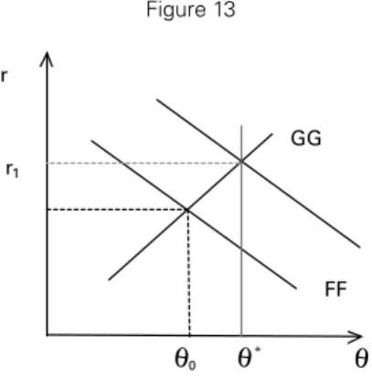
What are the options that the Monetary Authority and the Treasury have at their disposal to produce a depreciation of the real exchange rate in order to achieve the industrial equilibrium? A first option is to increase the level of capital controls, which implies a reduction of the value of
l
in equation (9). In this case, there will be a re-duction in demand of non-residents by domestic bonds11. Given the amount of bonds issued by the Treasury and the amount of the same type of bonds in the Central Bank’s portfolio, this will result in an oversupply in bond market. To restore equilibrium in the bond market is necessary an increase in domestic interest rates, which will shift the FF curve up and to the right as seen in Figure 13. Everything else constant, there will be an increase in the real rate of interest and a depreciation of the domestic real exchange rate. If the reduction in the demand of domestic bonds by non-residents due to the increase of capital controls is strong enough, then the actual rate of ex-change may adjust to the level compatible with the industrial equilibrium.Figure 13
FF r
GG
r1
θ θ0 θ
*
This policy, however, has the side effect of an increase in real domestic interest rate, which discourages investment in fixed capital. Therefore, it is necessary to combine the introduction and/or increase of capital controls with a policy of fiscal contraction, which will allow a reduction in the real rate of interest without preju-dice to the attainment of the goal of real exchange rate.
As seen in Figure 14 the combination between capital controls and fiscal contrac-tion allows that the real exchange rate to be devalued until reaching the level given by industrial equilibrium without any negative impact on the real rate of interest.
Figura 14
FF0 r
GG0
FF1 GG1
GG2
θ θ0 θ
*
An important observation regarding Figure 14 is that it shows us that the com-bination between capital controls and fiscal adjustment may be politically more palatable to society in order to control the real exchange rate than only the fiscal adjustment. In fact, if the only instrument available to the policy makers is the fis-cal policy, the fisfis-cal adjustment required to produce a devaluation of the real ex-change rate to the level industrial equilibrium will be much greater than the re-quired in the case that the fiscal adjustment is combined with an increase of capital controls intensity. Indeed, keeping unaltered the level of capital controls, the GG curve needs to move up to GG2 to which the real exchange rate reaches the indus-trial equilibrium, while combining the fiscal contraction with an increase of capital controls intensity the GG curve only needs to move up to GG1.
In the exercise performed above the nominal exchange rate was assumed con-stant during the entire experiment. This means that real exchange rate depreciation was achieved through a reduction in the domestic price level or, in the case of a model in which prices grow at a sustained rate over time, through a disinflation.
CONCLUSION: A PROPOSAL FOR A MACROECONOMIC FRAMEWORK FOR BRAzILIAN CATCHING-UP
The empirical evidence presented in the previous sections have pointed to the fact that both the level and volatility of the real exchange rate in Brazil adversely affects the industrial investment decisions, which prevents, therefore, a more robust expansion of productive capacity and labor productivity without which it is impos-sible to accelerate sustained growth of the Brazilian economy. In addition, pre-liminary calculations on the level of the real exchange rate that would recover the level of competitiveness of Brazilian industry show that the real effective exchange rate is overvalued, probably around 48%. This is a significant overvaluation.
As we have seen in the previous section, the correction of an overvalued ex-change rate can be performed through the combination of an increase in the level of capital controls with a fiscal adjustment. As the international scenario in the next years must be characterized by a gradual adjustment in monetary liquidity condi-tions in developed countries, thus imposing an increase in international interest rates, which has similar effects to an increase in the level of capital controls, it fol-lows that tightening controls on the entry of foreign capitals can be discarded. Thus, the implementation of a fiscal contraction will be essential for obtaining a more competitive exchange rate.
This fiscal adjustment should be performed in the context of a reform of the fiscal regime in Brazil. Currently the fiscal regime is characterized by achieving a primary surplus target, which has been sufficient to stabilize the public debt/GDP ratio, but has not allowed a substantial increase in public savings, thus contributing to maintain low governments investments. In this way, we suggest the implementa-tion of a tax regime based on the goal of government current account surplus (see Oreiro, 2014). The implementation of this regime, necessarily requires the control of pace of growth of government expenses in consumption, thus enabling the fiscal adjustment required to obtain a more competitive exchange rate without deleteri-ous effects on the level of the real interest rate.
REFERENCES
ASTERIOUS, D; HALL, S. (2011). Applied Econometrics. 2a Ed. Palgrave.
ATESOGLU, H.S. (1997). “Balance of payments-constrained growth model and its implications for the U.S”. Journal of Post Keynesian Economics, Vol. 19, N.3.
BEAN, C. (1981). “An econometric model of manufacturing investment in the UK”. Economic Journal, vol. 91, pp. 106-21.
BONELI, R; BACHA, E. (2013). “Crescimento econômico revisitado” In: Veloso et al (orgs). desenvol-vimento econômico numa perspectiva brasileira. Campus: Rio de Janeiro.
BRESSER-PEREIRA, L.C; OREIRO, J.L; MARCONI, N. (2013). “a theoretical framework for structu-ralist development macroeconomics”. Anais do 41° Encontro Nacional de Economia, Foz do Iguaçu.
DARBy, J., HALLETT, A. H., IRELAND, J., PISCITELLI, L. (1999). “The impact of exchange rate uncertainty on the level of investment”. The Economic Journal, 109: 55–67. doi: 10.1111/1468-0297.00416
DIxIT, A. (1989). “Entry and exit decisions under uncertainty”. Journal of Political Economy, vol. 97, pp. 620-38.
EDWARDS, S. (2006). “The relationship between exchange rates and inlation targeting revisited”.
National Bureau of Economic Research Working Paper, nº 12163.
ELLERy, R; TEIxEIRA, A. (2013). “O milagre, a estagnação e a retomada do crescimento: as lições da economia brasileira nas últimas décadas” In: Veloso et al (orgs). Desenvolvimento Econômico numa Perspectiva Brasileira. Campus: Rio de Janeiro.
FERREIRA, P.C; VELOSO, F. (2013). “O desenvolvimento econômico brasileiro no pós-guerra” In: Veloso et al (orgs). Desenvolvimento Econômico numa Perspectiva Brasileira. Campus: Rio de Janeiro.
LEDESMA, M.L; THIRLWALL, A. (2002). “The endogeinity of the natural rate of growth”. Cam-bridge Journal of Economics, Vol. 26, N.4.
LIBANIO, G. (2009) “Aggregate demand and the endogeneity of the natural rate of growth: evidence from Latin American Countries”. Cambridge Journal of Economics, 33.
MONTIEL, P. (2011). Macroeconomics in Emerging Markets. Cambridge University Press: Cambridge. OREIRO, J.L; NAKABASHI, L; SILVA, G.J; SOUzA, G.J.G. (2012). “The Economics of Demand-Led
Growth: theory and evidence for Brazil”. CEPAL Review, N.106, Abril.
OREIRO, J.L. (2014). “Muito além do tripé”. Valor Econômico, 10 de janeiro de 2014.
_______ (2013). “A macroeconomia da estagnação com pleno-emprego no Brasil”. Revista de Conjuntu-ra, Corecon/DF, Ano xII, N.50.
_______ (2012). “Novo-Desenvolvimentismo, crescimento econômico e regimes de política macroeconô-mica”. Estudos Avançados, Vol. 26, N.75.
PARK, M.S. (2000). “Autonomous demand and the warranted rate of growth”. Metroeconomica. ROSSI, P. (2013). “Biruta no vento: descaminhos da lutuação cambial”. Valor Econômico, 30 de
se-tembro.
SOUSA, A; BASILIO, F; OREIRO, J.L. (2013). “Wage-led ou proit-led? Análise das estratégias de cres-cimento das economias sob o regime de metas de inlação, câmbio lexível, mobilidade de capitais e endividamento externo”. 41º Encontro de Economia – Anpec. Foz do Iguaçu.
TURNER, P e J VAN’ T dack (1993). “Measuring international price and cost competitiveness”. BIS Economic Papers, no 39, Basel, November.
Figure 7: Daily Volatility of the nominal exchange rate
Table 2: Analisys of Volatility of the Nominal Exchange Rate (daily)