OCTOBER 9,2003
DEBT COMPOSITION AND EXCHANGE RATE BALANCE SHEET EFFECTS IN BRAZIL: AFIRM LEVEL ANALYSISO
MARCO BONOMO* BETINA MARTINS** RODRIGO PINTO***
ABSTRACT
In this paper we study the interaction between macroeconomic environment and firms’ balance sheet effects in Brazil during the 1990’s. We start by assessing the influence of macroeconomic conditions on firms’ debt composition in Brazil. We found that larger firms tend to change debt currency composition more in response to a change in the exchange rate risk than small firms. We then proceed to investigate if and how exchange rate balance sheet effects affected the firms’ investment decisions. We test directly the exchange rate balance sheet effect on investment. Contrary to earlier findings (Bleakley and Cowan, 2002), we found that firms more indebted in foreign currency tend to invest less when there is an exchange rate devaluation. We tried different controls for the competitiveness effect. First, we control directly for the effect of the exchange rate on exports and imported inputs. We then pursue an alternative investigation strategy, inspired by the credit channel literature. According to this perspective, Tobin’s q can provide an adequate control for the competitiveness effect on investment. Our results provide supporting evidence for imperfect capital markets, and for a negative exchange rate balance sheet effect in Brazil. The results concerning the exchange rate balance sheet effect on investment are statistically significant and robust across the different specifications. We tested the results across different periods, classified according to the macroeconomic environment. Our findings suggest that the negative exchange rate balance sheet effect we found in the whole sample is due to the floating exchange rate period. We also found that exchange rate devaluations have important negative impact on both cash flows and sales of indebted firms. Furthermore, the impact of exchange rate variations is asymmetric, and the significant effect detected when no asymmetry is imposed is engendered by exchange rate devaluations.
JELCODE:E22,F31
KEYWORDS:BRAZIL,INVESTMENT, EXCHANGE RATE, BALANCE SHEET EFFECTS, CREDIT CONSTRAINTS.
o
A revision in the data set allowed us to obtain results that were different from those in Bonomo, Martins, and Pinto (2003). We thank Arturo Galindo, Campbell Harvey, Ugo Panizza, Fabio Schiantarelli for useful suggestions. We also received valuable comments from Heitor Almeida, Steve Bond, Kevin Cowan, Linda Goldberg, and Silvia Valadares. We also thank audiences of IDB seminars in Madrid and Boston, where preliminary versions of this paper was presented. We are grateful to Renata Werneck for excellent research assistance. Part of this paper was written when the first author was visiting CIRANO, CRDE (Université de Montréal) and the Bendheim Center for Finance (Princeton University).
*
Graduate School of Economics, Fundação Getulio Vargas. Address for correspondence: Praia de Botafogo 190/1110, Rio de Janeiro, RJ 22253-900, Brazil. E-mail: [email protected]
**
Fundação Telos.
***
1. Introduction
The macroeconomic environment interacts with the firms’ balance sheet structure in a two-way relationship. On one hand, macroeconomic environment is central in shaping the capital markets, determining what kind of contracts is feasible and enforceable. Moreover, it also affects the incentives faced by firms when selecting their financial contracts. Conversely, the firms’ balance sheet structure affects crucially the result of macroeconomic policies, influencing policymakers’ choices of regimes and policy rules. In this paper we study the balance sheet effects of exchange rates and interest rates in Brazil since 1990, using a panel data set with firm level variables. For this endeavor, we also consider how the macroeconomic environment affected the debt composition and interacted with firms’ level balance sheet effects.
Balance sheet effects on investment and production rely on capital market imperfections. According to the credit channel literature (see Bernanke and Gertler, 1995), imperfect information creates a wedge between internal and external finance. An adverse shock to the net worth of a financially constrained firm increases its cost of external financing and decreases the ability or incentive to invest, and to implement production plans. It should impact firms differently, being stronger for firms that face higher premium of external finance costs relative to internal finance (see Hubbard, 1998).
There is substantial empirical evidence that proxies for firms’ net worth affect investment more for low net worth than for high net worth firms (Hubbard 1998). Therefore, to the extent that exchange rate and interest rate variations affect firms’ net worth, their balance sheet effect should matter for determining investment. Firms will see their financial condition deteriorate whenever they have substantial debt at floating interest rates, and the relevant real interest rate increases. This can happen if they have foreign denominated debt and the real exchange rate depreciates, entailing an exchange rate balance sheet effect. An interest rate effect takes place when firms have substantial short-term domestic debt or long-term debt contracted at floating rates, since their loans will be rolled over at higher rates.
In the case of interest rates, it engenders a financial accelerator, which magnifies the traditional interest rate channel (Bernanke, Gertler, and Gilchrist, 1999). In the case of exchange rate, it should counteract the expansionary effect of the competitive channel
(Aghion, Bacchetta and Banerjee, 2001).1 Thus, while the question in the interest rate
literature is about the magnitude of the recessive impact of interest rate rises the debate in the recent exchange rate literature is about whether exchange rate devaluations are expansionary or contractionary.
Harvey and Roper (1999) argued, in an investigation which used firm level indicators, that the exchange rate balance sheet effect greatly exacerbated the Asian Crisis. Bleakley and Cowan (2002) and Forbes (2002) tested the empirical relevance of exchange rate balance sheet effects using multinational panel regressions with firm level data. The
1
former work used a panel data for over 500 non-financial firms in five Latin American countries, dominated by Brazilian firms (52.5% of the observations). They found that holding foreign-currency denominated debt was associated with more investment during exchange rate devaluations, contrary to the predicted sign. On the other hand, Forbes (2002) found that more indebted firms had lower net income growth after a large depreciation. Although she used a larger sample of countries, she only examined large depreciations.
One advantage of focusing in one specific country is that we can take into consideration the relevant specifics of the macroeconomic environment. The macroeconomic conditions changed drastically in the last 12 years in Brazil. First there was an important trade liberalization, which occurred in the early 1990’s. Simultaneously, the control of international financial flows was softened, increasing the access of Brazilian firms to foreign liabilities. The Real plan in 1994 ended the high inflation period in Brazil, unveiling the new incentives, and at the same time creating additional ones. The sudden reduction of inflation rate and its volatility contributed for the strengthening of credit relations and for the lengthening of debt maturities. This happened at first in an environment characterized by low volatility of the real exchange rate. In the beginning of 1999 the exchange rate was allowed to float. This change of exchange rate regime was complemented by the adoption of an inflation targeting monetary regime. As a result, exchange rate became very volatile while interest rate policy became focused on bringing inflation to target.
Our investigation evolves around two issues. The first topic we study is the determinants of debt composition, focusing on currency denomination and maturity. Then, we investigate the balance sheet effects of exchange rate devaluations and interest rates. The issues are interrelated since the balance sheet effects of exchange rate and interest rates depend on currency denomination and maturity of debt.
At firm level, investment is the candidate variable potentially more influenced by balance sheet effects. Balance sheet effects might additionally affect production. Since this variable was not available, we used sales as its proxy. Since firms cash flow could be an important channel through which balance sheet deterioration affect investment, we also investigate how cash flows affect investment (also a usual measure of capital market imperfection), and how they are influenced by our balance sheet effects.
inputs are added. There is also some weaker evidence that firms in industries with higher proportion of imported inputs invest less when the real exchange rate is more depreciated. We also test interest rate balance sheet effects, but we found no evidence of such an effect in our sample. We then investigate how the macroeconomic environment influenced our results. More concretely we allow exchange rate balance sheet effects to vary over the three periods we divided our sample. Our findings suggest that the negative exchange rate balance sheet effect we found in the whole sample is due to the floating exchange rate period.
We also explore the link between balance sheet effects and investment through a common test of capital market imperfection. In principle Tobin’s q could provide a better control for the competitiveness effect on investment since it should capture all investment opportunities. Our results provide evidence for imperfect capital markets, and for a negative balance sheet effect of exchange rate depreciations. Exchange rate depreciations could reduce cash flows and still have further effects on balance sheets. In order to get a more detailed account of those different channels we look into an additional effect of exchange rate variation on more indebted firms, even after controlling for cash flows. We found that the effect is smaller, but still statistically significant. On the other hand, we test if firms more indebted in foreign currency have lower cash flows during exchange rate depreciations. The effect is strong and highly statistically significant. Since it could be attributed both an increase in financial expenses and to a decrease in production, we also test for an exchange rate balance sheet effect on sales. Again we found a strong highly significant negative effect.
We also follow the capital market imperfections tradition by testing if the balance sheet effects are stronger for firms with characteristics that make them more likely to be financial constrained. The characteristics we test are size (market capitalization), foreign ownership, belonging to tradable sector, and having issued an ADR. None of those characteristics have a differential impact on the balance sheet effect.
Finally, we test if the effect of exchange rate variation on investment, cash flows and sales was asymmetric. We found that only depreciations have a significant differential impact on firms more indebted in foreign currency. The coefficients found for the interaction between exchange rate depreciation and debt in foreign currency was of the same order of magnitude of those found without discriminating between depreciations and appreciations.
2. Macroeconomic and Institutional Environment
The reforms in Brazil changed substantially the macroeconomic environment. This should affect the restrictions and incentives firms face when deciding how to finance their activities, and specially investment. The equity market in Brazil remained in the whole period as a marginal source of funds. Therefore, the sources of funds for investment were either retained profits or debt. Given the high level of interest rates, and the scarcity of long-term loans caused by the macroeconomic instability, the internal source was presumably very important.
Our period of analysis starts in the early nineties, when tariffs were substantially reduced. The average nominal tariff plunged from 39.6% in 1988 to 11.2% in 1994. Trade liberalization should make firm performance more sensitive to exchange rate, since it should play a more relevant role in determining the competitiveness of domestic tradable products. There was also an important financial liberalization that gave firms more access to foreign assets and liabilities. Among the important advancements in this direction we could cite the successful launch of an important privatization program, the reached agreement to restructure arrears on its external debt, and the approved new rules allowing foreign investment in domestic market and the financing of Brazilian firms in foreign markets (see Table 1). However, macroeconomic instability was still responsible for a reduced supply of foreign and domestic long-term credit.
In 1994, the Real plan succeeded in finishing the chronic inflationary process. Brazil has had one of the world’s longest high inflation processes (see Figure 1B). Long-term debt and financial assets had practically disappeared, and even shorter-term financial instruments had become indexed to the inflation rate or to the daily interest rate. Low inflation coupled with new financial regulation which outlawed indexation provided a completely new environment for financial decisions, resulting in increased debt maturity and reduced indexation.
From July 1994, and 1998, with exception of the initial eight months where it was let to appreciate (see Figure 1C), the exchange rate was controlled and stable, as the Central
Bank was committed to prevent any abrupt devaluation2. The successful stabilization
contributed to a substantial increase in the flow of foreign investments. However, the recurrent emerging markets crises would make the flow cyclical. As a response, the government changed cyclically the legislation, reducing the incentives to capital inflows in the good times, and undoing it in the bad times. Few months after the stabilization, the Mexican crisis hit capital inflows to Brazil severely. The situation was reversed in the second semester of 1995. From then on, external debt became a relatively important source of financing for large firms, subject to cyclical interruptions in the new flows caused by the succession of emerging markets crisis.
2
When uncertainty about the sustainability of the crawling-peg exchange rate regime increased, firms started to hedge against the exchange rate devaluation risk. In January 1999, exchange rate was allowed to float. As a complement to the floating exchange rate regime, the Central Bank adopted an inflation-targeting framework for monetary policy in June. As a result exchange rate became much more volatile, although interest rate became less volatile. Under the free-floating regime, the risk of adoption of capital controls was reduced, which stimulated further the supply of foreign credit.
In this environment firms had more incentive to bear interest rate risk and to hedge exchange rate risk. There are several instruments for hedging exchange rate risks in the Brazilian economy, such as exchange rate futures contracts, dollar indexed government bonds, swaps, dollar currency, foreign assets, etc. In the recent period, a frequent hedging mechanism used by firms is the acquisition of swaps from banks involving the exchange of interest in domestic currency for dollar-indexed payments. This mechanism is preferred because banks make tailor-made contracts according to the firm’s necessity. On the other hand, banks are not exposed to exchange rate risk because they have dollar indexed government bonds in their portfolios. Thus, in net terms, hedge is provided by government, with banks’ intermediation.
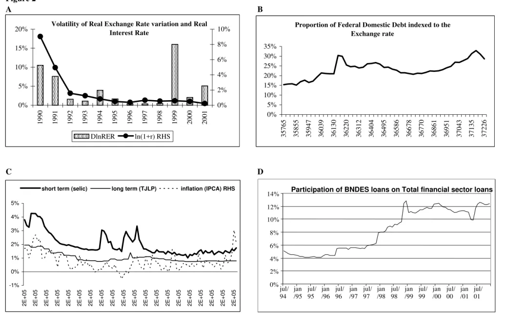
In Figure 2B, we can see that the proportion of the domestic federal debt securities indexed to the exchange rate more than doubled in 4 years, increasing from about 15% in December 1997 to about 33% in December 2001. This figure underestimates the increase in hedge since the Central Bank also offered exchange rate swaps attached to domestic currency.
Another important aspect is that, because of the macroeconomic instability, there is no private supply of run loans for investment in Brazil. The main provider of long-term loans is the Brazilian National Development Bank (BNDES). These loans were indexed to inflation before stabilization. After the Real plan, inflation indexation with fixed interest rate was substituted by floating interest rate (named TJLP). This interest rate is decided by the National Monetary Council with base on the inflation target and Brazil’s risk premium, and is lower and more stable than the market rates (see Figure 2C.). Figure 2D shows the proportion of BNDES loans in total loans to the private sector. It amounted to more than 12% of the total loans of the financial system at the end of 2001, which should correspond to a very large part of the long-term domestic loans.
investment rate, as a capital stock ratio, remained stable around 5% (Figure 1D): a mediocre rate engendered by the unstable macroeconomic environment.
3. Database Description
This section describes the sample and variables under study. Our main data consists of firm-level accounting information for Brazilian non-financial corporations and country-level data, organized as a panel data set. The time period under investigation
ranges from 1990 to 2002, with yearly observations.3
We started by using balance sheet data of a large sample of firms provided by Austin Asis of listed and unlisted companies. The use of the whole data set for investigating the above issues was not fruitful, possibly because unlisted firms balance sheets are not required to be audited in Brazil. Then, we decided to restrict our investigation to open firms, using both the Austin Asis and Economatica data sets to construct our variables of
interest and enlarge the number of observations in each regression.4
Additionally, we have data describing the firm’s ownership structure and reported ADR issues collected from CVM, as well as measures of export orientation (exports/production) and imported inputs at industry level obtained at the FUNCEX.
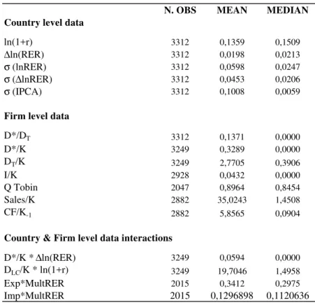
In Table 2 we report the number of observations in the sample per year, which remains stable with an average of 263.3 firms per year. In Table 3 we report the mean and median for the variables (and its interactions) under estimation.
Our main dependent variable is Investment, measured as the change in net property
and equipment added depreciation.5 During the estimation procedure, all firm variables
were calculated as ratios to capital stock measured as the net property and equipment at the beginning of the year. In the appendix we describe all the variables used in detail.
4. Analysis of the debt composition
The first topic we study is the determinants of debt composition, focusing on currency denominated and maturity.
3
Quarterly accounting numbers and monthly market variables are available and used in the construction of some variables.
4
We used capital and debt variables from Austin and the remaining ones from Economatica. The number of observations in each regression was much smaller in earlier versions, where the balance sheet data were based only on Economatica.
5
4.1Methodology
In order to investigate the factors determining the changes in debt composition, we
estimate equations for the ratio of dollar-debt D* over total debt D, and of long-term debt
DLT over total debt D. We estimated the following equation:
it t it it
t
it c m f f y
r = +α⋅ ⋅ +β⋅ + +ε
where rit is a debt ratio, mt’s are variables capturing the macroeconomic environment
and fit’s are firms’ individual features.
As rit is necessarily between zero and 1, the distribution of the right hand side variable is
truncated, and tends to have atoms in the limits. We chose to estimate a Tobit model, which is an appealing specification when the range bounds have a relatively large proportion of observations. We checked that this is the case in our sample.
This equation is a reduced form and should reflect factors influencing both the demand and the supply for loans.
With imperfect capital markets, supply of funds becomes a relatively more important determinant of the debt composition. In particular, the availability of external funds depends on the liquidity of the international capital markets and on the international assessment of the country risk. Thus, the foreign supply of external debt is a key determinant of the dollar debt.
Finally, given the high level of interest rates, and the scarcity of long-term loans caused by the macroeconomic instability, the firms’ internal savings were presumably a very important source of funds for investment, especially before the stabilization.
For the foreign debt ratio equation we chose m as volatility of real exchange rate, and interacted it with size (proxied by log K). When r is the log-term debt ratio we chose m as volatility of inflation, and also interacted it with as size (log K). We also tested the direct effect of having an ADR, being a foreign-owned firm, and belonging to the tradable sector. One would expect that volatility of RER would affect the risk of foreign debt, and that volatility of inflation would affect the risk of long-term debt. It is also expected that large firms have a better access to financial markets, and therefore could change their portfolios in response to a change in risk. Therefore one would expect that an increase in the volatility of real exchange rate would reduce more the demand of foreign debt by large firms. Similarly an increase in the volatility of inflation would reduce more the demand for long-term loans by large firms. In terms of the equation above, if demand is
the prevailing effect on the debt rations, the coefficient α in both equations should be
negative. We also expect a positive coefficient for the direct effect of our size proxy (log K), and for the ADR dummy, since a larger firm and a firm that issued an ADR should be better access to the restricted foreign and long-term loan markets. One would also expect a positive coefficient for the foreign ownership and tradable sector dummies in the equation for the foreign currency debt ratio, since firms with those features have a better matching in terms of risk with foreign currency liabilities.
4.2Results
Table 4 reports the results of our Tobit regressions for the ratio of debt in foreign currency to total debt. In the first column we have only size and the interaction between the volatility of the real exchange rate and size as explanatory variables. The coefficient of the interaction between the volatility of the real exchange rate and size has the negative expected sign and is highly statistically significant. This can be interpreted as meaning that larger firms are more able to reduce foreign debt when its risk increased. The size variable has also a statistically significant positive coefficient, which is expected sign. Those results are maintained in the other regressions, when we add other firm level controls. In the second column we add a dummy for firms with ADR’s. The ADR dummy has the positive expected coefficient, statistically significant at 1%, a result which is maintained in other regressions. In the third column we add a dummy for foreign owned firms and in the fourth we also include a dummy for firms in the tradable sector. The coefficients of the foreign ownership and tradable dummies are not significantly different from zero.
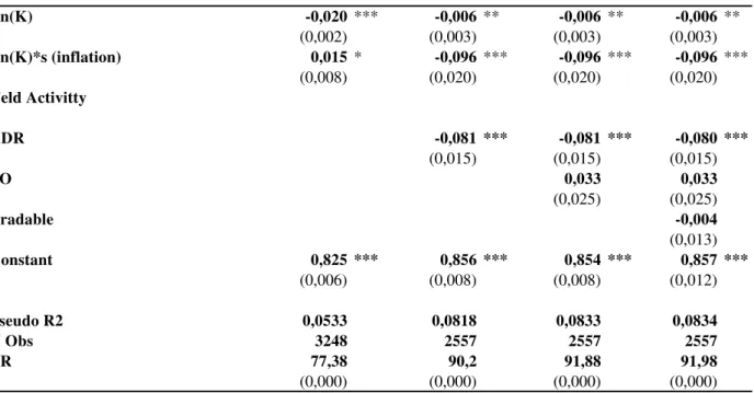
controls, this coefficient becomes negative and statistically significant at 1%. This is the expected sign, meaning that a larger firm is less likely to have long-term debt when inflation is higher. Both the coefficients of the size variable and of the ADR dummy are always negative and statistically significant, while the foreign ownership and tradable dummy coefficients are never significantly different from zero. The interpretation of some of those results is more troublesome. This is because in Brazil the National Development Bank is the main provider of long-term loans, and those loans tend to be subsidized. Then, the results could reflect more government policy than firms’ choices. The negative sign of the size and of the ADR value could mean that the government favors smaller firms, without access to international financial markets.
5. Investment and Balance Sheet Effects
Bleakley and Cowan (2002) investigated the balance sheet effect of exchange rate using a sample where more than a half of observations were due to Brazilian firms. They found that the effect of an exchange rate devaluation was positive and statistically significant, which implies that balance sheet effects are not important. We intend to investigate this result by running different specifications of the investment equation.
We start by testing directly the balance sheet effects in some basic dynamic panel regressions. Then, we look at the role of capital market imperfections, firm heterogeneity, and macroeconomic environment.
In estimating the dynamic panel regressions below, we could not use an OLS estimator, since it will be seriously biased due to correlation of the lagged dependent variable with the individual specific effects. A usual technique for dealing with variables that are correlated with the error term is to instrument them.
5.1. Direct tests
5.1.1 Basic regressions
Our strategy is to test first directly for the balance sheet effect of the exchange rate by running the following regression,
t i i t t i t i t i t i t t i t i t i t i t i t i K D K D RER K D K I K I , 1 , 1 , 1 , 1 , * 1 , 1 , * 2 , 1 , 1 , , )
ln( δ ϕ η µ ε
γ
α + ∆ + + + + +
= − − − − − − − − − (1)
where Iitis the firm’s investment, RERtis the real exchange rate, ηt are year dummies
and µi firms fixed effects. Our main focus is on the coefficient of the interaction between
the real exchange rate depreciation and the debt in foreign currency. The total debt and debt in foreign currency are firm level controls. The year dummies intend to capture the variation of the macroeconomic environment through time.
If this equation captures an exchange rate balance sheet effect, one would expect a negative coefficient for the interaction between the foreign currency debt and exchange rate devaluation. The interpretation is that exchange rate devaluations affect more adversely a firm with higher foreign debt. A necessary condition for this effect is the existence of capital market imperfections. When a positive sign is found, the usual interpretation (Bleakley and Cowan, 2002) is that an exchange rate devaluation also entails a positive substitution effect, due to higher exports profitability, and that a firm with higher external debt is also more likely to experience a larger impact from this effect. When a negative coefficient is found, one could also attribute it to a negative substitution effect, which appeared because of the importance of imported inputs for the firms in the sample, if higher external debt and importance of imported inputs are related. In order to control for those effects, one could add exchange rate interactions with exports and imports in our explanatory variables. Since we did not have the proportion of exports and of imported inputs at firm level, we used industry level data for those variables.
5.1.1 Results of direct tests
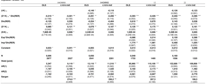
negative and statistically significant at 1% and at 5%, for the GMM estimations and for the others, ranging from -0.33 to -0.39. This suggests the existence of exchange rate balance sheet effects. The external debt is also positive and statistically significant at 5% for all estimations and at 1% for the GMM. This indicates that investment is positively related with a higher level of external debt in Brazil, which could be a reflex of the underdevelopment of the domestic long-term capital markets. The time-dummies are jointly statistically significant at 1% in all four equations.
The next four columns report the results of equivalent estimations for the dynamic specification. The coefficients of the interaction variable continue to be negative, and are significant at 5% in the OLS and within-group estimations, at 1% at the GMM difference estimation, and not significant in the GMM system estimation. The coefficient of external debt is also positive and statistically significant in three of the four equations. The coefficient of lagged investment is negative in all four regressions, what is consistent
with the results obtained in Terra (2003), and Ferrua and Menezes (2002)6. The
coefficient is statistically significant in the OLS and within-groups estimations, but not in the GMM estimations. Time-to-build aspects tend to generate positive correlation in investment. However, investment is also characterized as lumpy and intermittent, due to kinky adjustment costs (see Caballero and Engel,1999, Dorns and Dunne, 1993). This
latter aspect may lead to negative correlation7. Notice that the GMM specifications do not
pass the Sargan test.
The negative results obtained for the coefficient of the interaction between the dollar debt and exchange rate devaluation could also reflect a negative competitiveness effect of a higher proportion of imported input in the firms with higher external debt. Because of this, we add the interactions of multilateral exchange rate with sector exports and with input sector imports in the basic specification (equation 1), in order to capture the competitiveness effect, hoping that the coefficient of the interaction of exchange rate devaluation with foreign currency debt would now reflect mostly the balance sheet effect. The results are reported in the first column of table 7. The export interaction coefficient is positive, but not statistically significant. The import interaction coefficient is negative and statistically significant at 10% level, indicating that firms that import more inputs tend to reduce their investment more when there is an exchange rate devaluation. The coefficient of the interaction between exchange rate devaluation and debt in foreign currency is still negative, and now it is significant at 1% level. The specifications now pass the Sargan test. Notice that the magnitude of the gamma coefficient decreased slightly, what could suggest the interpretation that the coefficients in the estimation before were inflated by the negative competitiveness effect of imported inputs participation.
6
One could think that the negative coefficient is obtained because the all the three mentioned papers calculate investment from capital stock data. However, in earlier stages of our work we obtained the same negative coefficient when we used capital expenditures data as investment. Capital expenditure is available from Economatica but not from Austin. Its use limited severely our sample size.
7
The interaction coefficient estimate in the GMM dynamic regressions with control for exports and imports effects is -0.26. We could interpret this coefficient as representing the exchange rate balance sheet effect. Thus, if we assume that the coefficient is -0.25 for example, it would indicate that a devaluation of 10% reduces investment in 2.5% of the magnitude of the dollar debt, which can be a very sizeable effect.
In the second column we have cash flows and sales as additional controls, but not the export and import interaction terms. Both sales and cash flow coefficients are not
statistically significant. The coefficient of the interaction between exchange rate
devaluation and debt in foreign currency is still negative and significant at 5%. However, the specification does not pass the Sargan test. In the last column we add the export and import interaction terms to this specification. The sales and cash flow coefficients are still not statistically significant, and neither are coefficients of export and import interactions. However, the coefficient that represents the exchange rate balance sheet effect has its significancy increased, and the specification now passes the Sargan test.
Finally one could also argue that those controls do not capture an important part of the substitution effect, because this should also be important for firms producing for the domestic market. For example, a devaluation should increase protection for domestic producers of tradable goods, and allow them to have a higher profit margin. As a consequence, they would be more stimulated to invest. We will return to this issue in the next subsection.
Bleakley and Cowan (2002) found a positive and statistically significant coefficient for gamma in a sample dominated by Brazilian firms, which is in contrast with the result we found. They ran a slightly different regression. For comparison purposes we also ran some of the same regressions they ran, which include the direct effect of an exchange rate devaluation in the right-hand side. In the appendix we present the results for their static specification, and of a dynamic version, where we use the GMM difference estimation method to control for endogeneity of the explanatory variable. We also added the interaction terms involving sector imports and exports as explanatory variables but interacting with devaluation of the real bilateral exchange rate, as they did. We ran the regressions using the whole sample and using the 1991-1999 subsample, which corresponds to the years of their sample. In all regressions with the whole sample we found a negative and significant coefficient, ranging from about -0.40 to -0.30. In the restricted sample the results are positive and not significantly different from zero for the regressions without export and import controls. When we add the import and export interaction terms as explanatory variables, our main coefficient of interest become negative for the GMM estimations, and significant at 10% level for the static specification.
Another minor factor is the estimation method. When we estimate their equation using their restricted sample by GMM we found a negative coefficient, although not as statistically significant as the results we found for the whole sample.
5.2 Interest rate effects
Interest rates in Brazil were particularly volatile during the period exchange rates were controlled. A domestic interest rate increase could cause deterioration in the balance sheet of locally indebted firms, leading to a decrease in investment. In parallel to our tests of the exchange rate balance sheet effect, we ran a similar equation but with local currency debt in the place of dollar debt and real interest rate in the place of real exchange rate devaluation:
: t i it
t i t i t i t i LB t t i t i LC t i t i t i t i K D K D r K D K I K I , 1 , 1 , 1 , 1 , 1 , 1 , 2 , 1 , 1 , , )
ln( δ ϕ η µ ε
γ
α + + + + + +
= − − − − − − − − −
where LC
D is the debt in local currency and r is the domestic real interest rate.
The results, for a GMM difference estimation, are reported in the first column of table 8. The interaction term is not significantly different from zero. The domestic debt and the total debt coefficients are statistically significant at 1% with symmetric coefficients. The coefficient of total debt is about 0.12 and that of the local debt about -0.12. We can interpret these findings as reflecting the importance of the omitted debt foreign debt variable for investment. This assessment is reinforced by the fact that 0.12 is also the order of magnitude of the coefficient of external debt in tables 6, and 7, whereas the total debt coefficient is not significantly different from zero.
In the second column we add sector imports and exports interactions with multilateral exchange rate. The results do not change. In additional the input imports coefficient is negative and statistically significant at 5%. In the third column we have both exchange rate and interest rate interaction terms and foreign currency debt and local currency debt as additional controls. The exchange rate interaction term is negative and statistically significant at 1% level, but the interest rate interaction term is not significantly different from zero. The external debt coefficient is about 0.12 and is statistically significant at 5%, whereas the internal debt term is close to zero and insignificant. This reinforces the interpretation of the paragraph above, that the only type of debt that is correlated with investment is the debt in foreign currency.
5.3 Macroeconomic environment and balance sheet effects
that we take the period of 1995 to 1998 as our basis period and add slope dummies for the balance sheet effects in the high inflation (1990-1994) and floating exchange rate (1999-2001) periods.
In the first column of table 9 we report the results for the interaction between exchange rate devaluation and debt in foreign currency. The result for the base period is not significantly different from zero. The additional effect for the floating exchange rate period is negative and statistically significant at 1%, indicating that the effect we found in the regressions for the whole period is due to this subperiod. Furthermore, the coefficient for floating period (which is the sum of the coefficient for the base period plus the slope dummy coefficient for this period) is of the same order of magnitude of the coefficient found before for the whole period. When we add controls for the competitiveness effect (exports and imports interactions) the results are not qualitatively affected, as seen in the second column. Then we let both exchange rate and interest rate interactions to be different in subperiods. The results for the exchange rate interaction are maintained, and all coefficients related to the interest rate effect are insignificant.
The exercise just proposed is based on particular priors of when the effects changed. Alternatively we allow for a different effect of dollar debt for each year. In this case, if we divide the obtained coefficient by the exchange rate variation, we could obtain the coefficient of the interaction between exchange rate devaluation and dollar debt for each year. If these coefficients are constant, the points in the plot of debt coefficient for a year versus exchange rate depreciation in the same year should be along a straight line.
The results are shown in the fourth column. We see that there are only two coefficients significantly different from zero. Those are positive coefficients, and correspond to the years of 1996 and 1998. In those years, there were only moderate changes in the exchange rate, and in opposite directions. However, we have identified two effects linking investment to external debt: a positive effect, related to investment financing, and a negative balance sheet effect. Those two effects cannot be disentangled in this experiment. The significant positive coefficients of 1996 and 1998 probably reflect the former effect.
5.4 Capital market imperfections 5.4.1 Main insights
With perfect capital markets investment is determined without reference to financial factors. A standard formulation is due to Hayashi (1982), where investment demand is
related to Tobin’s q8 – the ratio between investment market value and its replacement
cost. Balance-sheet effects should be relevant for firms’ investment when market imperfections create a wedge between the cost of internal and external finance. Then, if a
8
firm’s net worth is reduced the external finance premium increases, affecting negatively investment (see Bernake and Gertler, 1995). As a consequence, a proxy for net worth should affect investment, given the same financial opportunities, which are captured by q.
For our purposes, controlling for q could be more fruitful, because under certain conditions all variables that could affect the profitability of investment can be subsumed in q. If an exchange rate devaluation improves investment opportunities, for example, q should be increased. Then q should increase with a devaluation for an export firm, and also for a firm which produces tradable goods for the domestic market. Conversely a devaluation should cause a decrease in q for a non-tradable firm largely dependent on imported inputs. Therefore, this control should be able to capture the competitiveness effect more widely than the ones based on exports and imported inputs. Another advantage is that q, being a forward-looking variable dependent on expectations, could also reflect the extent to which a devaluation is believed to be temporary or permanent.
As we argued before, investment could be reduced when there is an exchange rate devaluation if a firm suffers financial distress because it is largely indebted in dollars, and this is the main effect we want to assess. However, this outcome depends on the existence of capital market imperfections. If capital markets were perfect the balance sheet effect would not occur even if the firm were heavily indebted in dollars. Therefore, tests for capital market imperfections are intrinsically related to tests for balance sheet effects. In the financial literature q has a crucial role in the tests for capital market imperfections, because it is considered a good control for investment opportunities.
On the other hand, the so called competitiveness effect on investment should be entirely captured by q. Then, controlling for q should allow us to separate the competitiveness and balance sheet effects. Therefore, in this context there is no further need of other terms related to export and import orientation or tradability in order to capture the competitiveness effect.
A usual proxy for net worth in the investment literature is cash flow.9 Despite the
importance of cash flow for investment, it does not capture in principle all the net worth effect of an exchange rate change variation. Although exchange rate devaluations tend to increase financial expenses of firms indebted in dollars, therefore affecting cash flow directly, it also increases debt. Thus, as shown by Bleakley and Cowan (2002), the increase in current expenses is only a part of the negative effect on net worth.
We start with a test of capital market imperfections - which is a necessary condition for a balance sheet effect - by evaluating the effect of cash flows on investment, after controlling for q. We run the following regression:
9
t i i t t i it it t i t i t i t i K CF q K I K I , 1 , 2 , 1 , 1 ,
, = α + λ + θ + η + µ + ε
− − − − (2)
where qit and CFit are firm’s i Tobin’s q and cash flows at time t, respectively, and the
other variables are as in the equation before. A positive and significant coefficient λ may
be interpreted as evidence of capital market imperfections.
Then, we test for exchange rate balance sheet effects on investment using q to control for competitive effects. We run the regression:
t i i t t i t i it t i t i t i t i RER K D q K I K I , 1 , 1 , * 2 , 1 , 1 , , )
ln(
µ
ε
γ
λ
α
+ + ∆ + += − − − − − (3)
We also add external debt and leverage as controls.
We then proceed with a more detailed investigation on the specific channels for the exchange rate balance sheet effect. First, we test if there is an effect of exchange devaluation for firms highly indebted in dollars, even after controlling for cash flows. We then add leverage and external debts for a more complete set of financial related controls.
It is natural to think that if exchange rate balance sheet effects are important, exchange rate depreciation will affect more negatively the cash flow of indebted firms. This could be the channel through which an exchange rate devaluation has a negative balance sheet effect on investment. In order to test this hypothesis we run the following regression: t i i t it t it t t i t i t i t i t t i t i t i t i t i t i M MRER X MRER K D K D RER K D K CF K CF , 2 , 1 , 2 , 1 , * 2 , 1 , * 2 , 1 , 1 , , ) ln( ε µ η κ η δ ϕ γ α + + + ⋅ ⋅ + ⋅ ⋅ + + + ∆ + = − − − − − − − −
− (4)
where MRER denotes the multilateral real exchange rate, X the sector exports, and M the sector imports. As before, we added import and export terms to control for the competitiveness effect. However, cash flow is not only a financial variable. A firm in the tradable sector could benefit from the devaluation and produce more, despite having dollar debt and also being negatively affected by the devaluation. The effect on cash flow could be ambiguous in this case. On the other hand, we one may also be interested in investigate if there is a negative exchange rate balance sheet effect in production. Since there is no production, we ran an equivalent (to equation 4) regression for sales.
5.4.2 Main results
q variable is not statistically significant, but the coefficient of cash flow is positive and statistically significant at 1% level. This could be interpreted and evidence in favor of imperfect capital markets, corroborating the findings of Terra (2003) for Brazil.
The existence of imperfect capital markets is a necessary condition for the exchange rate balance sheet effect. Thus, the next question is that if using q as a control for investment opportunities, which includes the competitiveness effect, we can capture the balance sheet effect. Thus, in the second column we run regression (3). The
coefficient of the dollar debt-exchange rate interaction is positive, but is not statistically different from zero. We then add external debt and leverage as additional controls. Then, the coefficient becomes negative and statistically significant at 1%. In order to investigate how much of the balance sheet effect is related to cash flow, we finally add cash flow as an additional control. Then the magnitude of the dollar debt-exchange rate interaction is halved and its degree of significance reduced to 10%. This suggests that an important part of the negative balance sheet effect happens through cash flow reductions.
In order to test this hypothesis we estimate equation (4), which has cash flow as the dependent variable. The results are shown in the first column of table 11. The coefficient gamma is negative and statistically significant at 1% level. Furthermore, its magnitude is about ten times the gamma coefficients found in investment equations. Since profits depend also on production, one may wonder if all this effect on cash flows come from higher finance expense or if production is reduced. He tried to answer this question by estimating equation (4) with sales in the place of cash flows. Our main effect is still negative and significant at 1% level, and its magnitude is now even higher.
5.4.3 Testing for heterogeneity
It is in the tradition of the literature of capital market imperfections to test for differential effects between group of firms. The idea is to select groups that have characteristics related to access to capital markets. Then a hypothesis to be tested, for example, is that if the investment of the group with presumably less access to capital markets is more sensitive to cash flows. A natural extension to our setting would be then to test if the balance sheet effect is stronger for those groups of firms. We estimate the equation: t i i t t i t i t i t i i t t i t i t t i t i it t i t i t i t i K D K D SD RER K D RER K D q K I K I , 2 , 1 , 2 , 1 , * 1 , 1 , * 1 , 1 , * 2 , 1 , 1 , , ) ln( ) ln( ε µ η δ ϕ ψ γ λ α + + + + + ⋅ ∆ + ∆ + + = − − − − − − − − − − −
where SD is a dummy that is equal to one if a firm is small. We then test if ψ is
where SD equal to one when the firm is of the tradable sector, has ADR, or it is owned by foreigners.
The results are reported in table 12. In the first columns we test for heterogeneity between small and large capitalization firms. The slope dummy coefficient has a positive sign, but smaller in magnitude than the gamma coefficient. This indicates that small firms still bear a negative balance sheet effect, but its intensity is smaller than the one faced by large firms, which is not the expected result. However, none of the coefficients are statistically significant, indicating a large dispersion within each group.
When the firms are divided according to the other criteria, the main effect continues to be negative and statistically significant at 1%. However, the it is not possible to reject the null that the two groups face the same effect.
5.5 Asymmetric effects of exchange rate variation
Our aim in this section is to test if there are asymmetric exchange rate balance sheet effects on investment, cash flows and sales. With this objective, we modify the basic regression (1) by decomposing the interaction between exchange rate variations and dollar debt into two effects: one for depreciations and another for appreciations. We repeat the experiment for cash flows and sales. The results are reported in table 13.
The depreciation interaction coefficients are negative, statistically significant, and have magnitude similar to the gamma coefficients we found when we did not
discriminate between depreciations and appreciations. The appreciation coefficients are not significantly different from zero. Those features emerge in all three estimations, which clearly indicate that the negative balance sheet effects we found were due to depreciations. This asymmetry reinforces the interpretation that the negative effect of the interaction between debt in foreign currency and exchange rate variation is due to balance sheet effects, since those appear more likely to be asymmetric than the ones related to competitiveness.
6. Macroeconomic Implications and Final Remarks
In our investigation we found a robust negative balance sheet effect of exchange rate depreciations on investment. The effect is due mostly to the period of floating exchange rate regime in Brazil. It also strongly impacts cash flows and sales, and is asymmetric, since only depreciations matter.
A question of natural interest is how important are the aggregate effects. Our sample is composed only by listed firms, which are relatively large in Brazil. The extrapolation of those results faces some difficulties. First, we do not have any measure of the indebtedness in foreign currency of the unlisted firms. We could speculate that the majority of those firms are smaller and do not have access to loans in foreign currency. We would be led conclude that the aggregate effect will be less important than the average effect in our sample. However, since the government is the net provider of hedge for the private sector, devaluations entail an additional negative effect, which is the deterioration of government’s financial health. In an emerging market economy, the composition of those two effects could make it prone to macroeconomic instability.
An interesting policy question is how to compare a crawling peg regime, such as the one between 1995 and 1998, to the free floating regime, from 1999 on. In the former, the instability and public accounts deterioration were generated by the high and variable level of interest rates necessary to control the exchange rate. In the floating regime, the risk should in principle be incurred by the private debtor, engendering exchange rate balance sheet effects that were not present in the crawling peg period. Those balance sheet effects ought to be attenuated when firms are partially hedged by the government, as it was the case in Brazil. However, as argued above, this government’s decision generates an additional channel of instability.
One could argue that the problem could be avoided in the free floating regime, if the government abstained from providing hedge to the private sector. Would we find then stronger exchange rate balance sheet effects? Without government intervention, hedge provided by the private sector would be substantially more expensive, and a firm before borrowing in foreign currency should take into account either the risk involved or the expensive cost of hedge.
References
Aghion, P., Bacchetta, P. and Banerjee, A. 2001. “Currency Crises and Monetary Policy
in an Economy with Credit Constraints”. European Economic Review. 45 (7): 1121-1150.
Arellano, M. and Bond, S. 1991. “Some tests of specification for panel data: Monte Carlo
evidence and an application to employment equations”, Review of Economic Studies 58:
277-97.
Bernanke, B. and Gertler, M. “Inside the Black Box: The Credit Channel of Monetary
Policy Transmission.” Journal of Economic Perspectives 9: 27-48.
Bernanke, B., Gertler, M. and Gilchrist, S. 1999. “The Financial Accelerator in a
Quantitative Business Cycle Framework”. In Handbook of Macroeconomics, vol. 1c,
Bleakley, H. and Cowan, K. 2002. “Corporate dollar debt and devaluations: Much ado about nothing?”. Mimeo. MIT.
Bonomo, M., Martins, B. and Pinto, R. 2003. “Debt Composition and Exchange Rate
Balance Sheet Effects in Brazil: A Firm Level Analysis.” Emerging Market Review
Bonomo, M. and Terra, C. 2001. “The Dilemma of Inflation vs Balance of Payments:
Crawling Pegs in Brazil, 1964-98.” In J. Frieden(Ed.) & E. Stein(Ed.), The Currency
Game - Exchange Rate Politics in Latin America. Washington: Inter-American
Development Bank, pp.119-155.
Caballero, R., and Engel, E. 1999. “Explaining Investment Dynamics in U.S.
Manufacturing: A Generalized Ss Approach.” Econometrica 67: 783-826.
Doms, M. and Dunne, T. 1993. “An Investigation into Capital and Labor Adjustment at Plant Level.” Mimeo. Center for Economic Studies, Census Bureau.
Ferrua Neto, L. and Menezes Filho, N. 2002. “Irreversibilidade de Custos e Decisões de
Investimento das Firmas Brasileiras.” In: Anais do Encontro Brasileiro de Econometria
Forbes, K. 2002. “How do large depreciations affect firm performance?”. NBER Working Paper 9095.
Hansen, L. P. (1982), “Large Sample Properties of Generalized Method of Moments
Estimators”, Econometrica, vol. 49, 1377-1398.
Hayashi, F. 1982. “Tobin’s Marginal q and Average q: A Neoclassical Interpretation.”
Econometrica 50: 213-224.
Harvey, C. and Hoper, A. 1999. “The Asian Bet,” in Alison Harwood, Robert E. Litan
and Michael Pomerleano, Eds., The Crisis in Emerging Financial Markets, Brookings
Institution Press, pp. 29-115.
Hubbard, G. 1998. “Capital-Market Imperfections and Investment.” Journal of Economic
Literature 36: 193-225.
Nucci, F and Pozzolo, A. 2001. “Investment and the exchange rate: An analysis with
firm-level panel data”. European Economic Review. 45: 259-283.
O Globo. 06/23/2002. “A ameaça do dólar nos balanços”. 33.
Reif, T. 2001. “The real side of currency crises”. mimeo. Columbia University.
Terra, C. 2003, “Credit Constraints in Brazilian Firms: Evidence from Panel Data,”
Figure 1
A
B
C D
Real GDP Growth (%)
-6% -4% -2% 0% 2% 4% 6% 8%
1990
1991
1992
1993
1994
1995
1996
1997
1998
1999
2000
2001
2002
Inflation - IPCA (%)
0%
500% 1000% 1500% 2000% 2500% 3000%
1990
1991
1992
1993
1994
1995
1996
1997
1998
1999
2000
2001
0% 5% 10% 15% 20% 25%
1995 1996 1997 1998 1999 2000 2001 2002
Multilateral Real Exchange Rate
Mult RER (R$/US$)
- 0,20 0,40 0,60 0,80 1,00 1,20
1990
1991
1992
1993
1994
1995
1996
1997
1998
1999
2000
2001
Investment/Capital
0% 1% 2% 3% 4% 5% 6%
1990
1991
1992
1993
1994
1995
1996
1997
1998
1999
2000
2001
Date Description
1990.03 - Collor Plan froze liquid financial assets creating a big liquidity squeeze (from 30% to 8% of GDP). Payments on government debt would be suspended for 18 months.
- Creation of a commercial market for foreign exchange rates transactions involving goods, complementing the floating market for restricted financial transaction.
1991.01 - 2nd Collor Plan: heterodox stabilization plan based on price freezing.
1991.05 - New and more orthodox economic team. Creation of the so-called Annex IV , which provided a channel for foreign investment in domestic security markets.
1991.07 - Rules for borrowing external resources though the ADR/IDR mechanism were adopted. 1991.09 - Devaluation of 14%
1991.11 - Privatization plan successfully started.
1992.09 - Impeachment of President Collor, replaced by Vice-President Itamar Franco
1993.05 - Fernando Henrique Cardoso was chosen Finance Minister. He and his team would formulate the Real Plan
1993.10 - First ADR was issued.
1994.05 - A new unit account URV was created to hyper-index the economy, as a preparation for the Real Plan
1994.07 - The new currency was created based on the URV, and inflation fell abruptly. De-indexation of contracts. Exchange rate was set an upper limit of 1, but no lower limit and was let to appreciate.
1994.10 - Fernando Henrique Cardoso elected president 1994.11 - Mexican crisis would affect capital inflows to Brazil.
1995.03 - Exchange rate band system was formerly adopted, with a band of 5%. Exchange rate was devalued in 5.2%.
1995.07 - Periodic exchange rate spread auction was started, establishing very narrow limits for exchange rate fluctuations.
1995.11 - As a response to the banking crisis caused by the dissipation of inflation tax, the government instituted a program known as PROER to facilitate the restructuring of the private banking sector.
1996.02 - US$8.2 billion bailout of Banco do Brasil
1996.10 - Financial transactions tax of 0.2% approved by the Congress. 1997.10 - Asian crisis affected capital flows to Brazil.
1998.10 - President Fernando Henrique Cardoso was reelected. 1998.07 - Russian crisis affected capital flows to Brazil.
1999.01 - The Central Bank announced 15% exchange rate devaluation on 01/14 and the creation of new band system. Currency was left to float three days later.
2000.06 - The Congress passed the Fiscal Reponsability Law restricting State and Municipalities ability to generate budget deficits.
2001.03 - Government reacted to energy crisis (low level of water stocks) imposing energy rationing. Contagion from Argentina crisis.
2002 - From May on deterioration of the international perception of Brazilian risk due to the prospect of a leftist government: sharp devaluation of currency and depreciation of Brazilian bonds.
Figure 2
A B
C D
0% 5% 10% 15% 20%
1990 1991 1992 1993 1994 1995 1996 1997 1998 1999 2000 2001
0% 2% 4% 6% 8% 10%
DlnRER ln(1+r) RHS
Volatility of Real Exchange Rate variation and Real Interest Rate
Proportion of Federal Domestic Debt indexed to the Exchange rate
0% 5% 10% 15% 20% 25% 30% 35%
35765 35855 35947 36039 36130 36220 36312 36404 36495 36586 36678 36770 36861 36951 37043 37135 37226
0% 2% 4% 6% 8% 10% 12% 14%
jul/ 94
jan /95
jul/ 95
jan /96
jul/ 96
jan /97
jul/ 97
jan /98
jul/ 98
jan /99
jul/ 99
jan /00
jul/ 00
jan /01
jul/ 01
Participation of BNDES loans on Total financial sector loans
-1% 0% 1% 2% 3% 4% 5%
1990 220
1991 207
1992 225
1993 262
1994 278
1995 279
1996 263
1997 277
1998 290
1999 271
2000 273
2001 251
2002 216
Total 3312
N. OBS MEAN MEDIAN
Country level data
ln(1+r) 3312 0,1359 0,1509
∆ln(RER) 3312 0,0198 0,0213
σ (lnRER) 3312 0,0598 0,0247
σ (∆lnRER) 3312 0,0453 0,0206
σ (IPCA) 3312 0,1008 0,0059
Firm level data
D*/DT 3312 0,1371 0,0000
D*/K 3249 0,3289 0,0000
DT/K 3249 2,7705 0,3906
I/K 2928 0,0432 0,0000
Q Tobin 2047 0,8964 0,8454
Sales/K 2882 35,0243 1,4508
CF/K-1 2882 5,8565 0,0904
Country & Firm level data interactions
D*/K * ∆ln(RER) 3249 0,0594 0,0000
DLC/K * ln(1+r) 3249 19,7046 1,4958
Exp*MultRER 2015 0,3412 0,2975
Imp*MultRER 2015 0,1296898 0,1120636
Table 3 - Descriptive Statistics
Table 4 - Estimation of Debt Currency Composition
Dependent Variable: Debt in Foreign Currency / Total Debt (D*/DT)
Ln(K) 0,135*** 0,094 *** 0,094*** 0,096 ***
(0,013) (0,013) (0,013) (0,014)
Ln(K)*σσσσ(∆∆∆∆lnRER) -0,906*** -0,677 *** -0,679*** -0,682 ***
(0,145) (0,159) (0,159) (0,159)
ADR 0,194 *** 0,193 *** 0,192 ***
(0,057) (0,057) (0,057)
FO -0,146 -0,150
(0,103) (0,104)
Tradable 0,030
(0,051)
Constant -0,441 *** -0,531 *** -0,522 *** -0,541 ***
(0,032) (0,041) (0,041) (0,052)
Pseudo R2 0,033 0,0251 0,0258 0,0259
N Obs 3248 2557 2557 2557
LR 136,3 81,36 83,39 83,75
(0,000) (0,000) (0,000) (0,000)
Table 5 - Estimation of Debt Maturity Composition
Dependent Variable: Long Term Debt / Total Debt (DLT/DT)
Ln(K) -0,020*** -0,006 ** -0,006** -0,006 **
(0,002) (0,003) (0,003) (0,003)
Ln(K)*s (inflation) 0,015* -0,096 *** -0,096*** -0,096 ***
(0,008) (0,020) (0,020) (0,020)
Yeld Activitty
ADR -0,081 *** -0,081 *** -0,080 ***
(0,015) (0,015) (0,015)
FO 0,033 0,033
(0,025) (0,025)
Tradable -0,004
(0,013)
Constant 0,825 *** 0,856 *** 0,854 *** 0,857 ***
(0,006) (0,008) (0,008) (0,012)
Pseudo R2 0,0533 0,0818 0,0833 0,0834
N Obs 3248 2557 2557 2557
LR 77,38 90,2 91,88 91,98
(0,000) (0,000) (0,000) (0,000) Standard deviation are in parentesis for parameters estimation.
P-values are reported in parentesis for test statistics. Tobit Model Estimation, the lower limit level is set to be 0. ∆Ln(K) means the difference of the log mean firm`s capital
Table 6
Dependent Variable: I/K
OLS WG GMM-Diff GMM-Sys OLS WG GMM-Diff GMM-Sys
(I/K) -1 -0,149 * -0,214 *** -0,110 -0,047
(0,08) (0,08) (0,14) (0,14)
(DFC/K) -1 * ∆∆∆∆ln(RER) -0,330 ** -0,391 ** -0,386 *** -0,379 *** -0,316 ** -0,356 ** -0,292 *** -0,241
(0,15) (0,17) (0,10) (0,13) (0,14) (0,14) (0,09) (0,20)
(DFC/K) -1 0,086 ** 0,109 ** 0,165 *** 0,114 *** 0,082 ** 0,101 ** 0,137 *** 0,062
(0,04) (0,05) (0,03) (0,04) (0,04) (0,04) (0,03) (0,07)
(DT/K) -1 2,11E-04 0,004 0,002 0,001 8,00E-05 0,001 0,002 0,000
(2,92E-04) (2,46E-03) (2,80E-03) (1,17E-03) (3,13E-04) (1,44E-03) (5,31E-03) (1,59E-03)
Constant 0,772 *** -1,018 *** 0,771 *** -0,010 0,031 -0,257
(0,229) (0,371) (0,229) (0,094) (0,139) (0,203)
R2 0,030 0,034 0,056 0,104
N 2877 2864 2527 2864 2541 2519 2201 2519
Wald (time) 41,450*** 36,660*** 35,510*** 45,230*** 28,330 *** 23,080 ** 25,270 *** 25,820***
(0,000) (0,000) (0,000) (0,000) (0,002) (0,010) (0,005) (0,004)
AR(1) -1,201 -1,556 -2,176** -2,211** 0,857 0,346 -1,479 -1,647*
(0,230) (0,120) (0,030) (0,027) (0,391) (0,729) (0,139) (0,100)
AR(2) -1,158 -2,145 ** -0,074 0,057 -0,653 -2,384 * -0,507 0,175
(0,247) (0,032) (0,941) (0,954) (0,514) (0,017) (0,612) (0,861)
Sargan 83,240 108,700 221,000 *** 267,900***
(0,986) (0,985) (0,000) (0,000)
Standard errors are in parentesis for parametrs estimation. P-values are reported in parentesis for test statistics.
The dynamic panel estimation uses GMM difference estimators, which are based on Arellano and Bond (1991). GMM results are one step estimates with heteroskedasticity-consistent standard errors and test statistics. GMM difference and system regressions use instruments lagged 2 to 6 periods in general.
AR(1) and AR(2) are tests for first-order and second-order serial correlation, asymptotically N(0,1). Time dummies are included in all equations.
Table 7
Dependent Variable: I/K
GMM Diff GMM Diff GMM Diff
(I/K) -1 -0,384 *** -0,105 -0,130
(0,047) (0,141) (0,091)
(DFC/K) -1 * ∆∆∆∆ln(RER) -0,262 *** -0,340** -0,308***
(0,075) (0,134) (0,093)
(DFC/K) -1 0,134 *** 0,107** 0,126***
(0,012) (0,045) (0,030)
(DT/K) -1 0,005 0,005 0,003
(0,004) (0,005) (0,004)
Sales/K 0,004 0,001
(0,003) (0,001)
CF/K -0,017 0,019
(0,012) (0,015)
Exp*MultRER 0,018 0,091
(0,24) (0,237)
Imp*MultRER -1,106 * -0,701
(0,589) (0,497)
Constant -0,252 ** 0,147 -0,049
(0,112) (0,282) (0,089)
N 1372 2200 1371
Wald (time) 14,630 22,300** 9,463
(0,146) (0,014) (0,489)
AR(1) -1,685 * -1,824* -1,851*
(0,092) (0,068) (0,064)
AR(2) -2,527 ** -0,358 -0,643
(0,012) (0,720) (0,521)
Sargan 186,800 268,800 205,200
(0,979) (0,132) (1,000)
Standard errors are in parentesis for parametrs estimation. P-values are reported in parentesis for test statistics.
The dynamic panel estimation uses GMM difference estimators, which are based on Arellano and Bond (1991). GMM results are one step estimates with heteroskedasticity-consistent standard errors and test statistics. GMM difference and system regressions use instruments lagged 2 to 6 periods in general.
AR(1) and AR(2) are tests for first-order and second-order serial correlation, asymptotically N(0,1). Time dummies are included in all equations.
Table 8
Dependent Variable: I/K
GMM-Diff GMM-Diff GMM-Diff
(I/K) -1 -0,148 -0,142 -0,114
(0,107) (0,094) (0,140)
(D*/K) -1 * ∆∆∆∆ln(RER) -0,334***
(0,129)
(D*/K) -1 0,117**
(0,048)
(DLC/K) -1 * ln(1+r) 0,001 -0,001 3,95E-04
(0,001) (0,001) (4,38E-04)
(DLC/K) -1 -0,115*** -0,125*** 0,003
(0,034) (0,023) (0,003)
(D/K) -1 0,121*** 0,135***
(0,035) (0,025)
Exp*MultRER -0,060
(0,228)
Imp*MultRER -1,275**
(0,527)
Constant -0,034 -0,036 0,005
(0,168) (0,052) (0,135)
N 2201 1372 2201
Wald (time) 25,830*** 16,020 * 24,900***
(0,004) (0,099) (0,006)
AR(1) -1,482 -1,601 -1,510
(0,138) (0,109) (0,131)
AR(2) -0,699*** -0,079 -0,484
(0,485) (0,937) (0,628)
Sargan 255,9*** 209,4 261,0**
(0,000) (0,988) (0,017)
Standard errors are in parentesis for parametrs estimation. P-values are reported in parentesis for test statistics.
The dynamic panel estimation uses GMM difference estimators, which are based on Arellano and Bond (1991). GMM results are one step estimates with heteroskedasticity-consistent standard errors and test statistics. GMM difference and system regressions use instruments lagged 2 to 6 periods in general.
AR(1) and AR(2) are tests for first-order and second-order serial correlation, asymptotically N(0,1). Time dummies are included in all equations.