remote sensing
ArticleMERIS Phytoplankton Time Series Products from the
SW Iberian Peninsula (Sagres) Using Seasonal-Trend
Decomposition Based on Loess
Sónia Cristina1,2,*, Clara Cordeiro3,4, Samantha Lavender5, Priscila Costa Goela1,2, John Icely1,6and Alice Newton1,7
1 Centre for Marine and Environmental Research (CIMA), FCT, University of Algarve, Campus de Gambelas, 8005-139 Faro, Portugal; priscila.goela@gmail.com (P.C.G.); john.icely@gmail.com (J.I.); an@nilu.no (A.N.) 2 Faculty of Marine and Environmental Sciences, University of Cadiz, Campus of Puerto Real,
Polígono San Pedro s/n, Puerto Real, 11510 Cadiz, Spain
3 Faculty of Sciences and Technology (FCT), University of Algarve, Campus de Gambelas, 8005-139 Faro, Portugal; ccordei@ualg.pt
4 Center of Statistics and Applications (CEAUL), Faculty of Sciences of the University of Lisbon, Bloco C6—Piso 4, Campo Grande, 1749-016 Lisbon, Portugal
5 Pixalytics Ltd., 1 Davy Road, Plymouth Science Park, Plymouth, Devon PL6 8BX, UK; slavender@pixalytics.com
6 Sagremarisco Lda., Apartado 21, 8650-999 Vila do Bispo, Portugal
7 Norwegian Institute for Air Research (NILU)-IMPEC, Box 100, 2027 Kjeller, Norway * Correspondence: cristina.scv@gmail.com; Tel.: +351-965-329-317
Academic Editors: Xiaofeng Li and Prasad S. Thenkabail
Received: 21 January 2016; Accepted: 19 May 2016; Published: 26 May 2016
Abstract: The European Space Agency has acquired 10 years of data on the temporal and spatial distribution of phytoplankton biomass from the MEdium Resolution Imaging Spectrometer (MERIS) sensor for ocean color. The phytoplankton biomass was estimated with the MERIS product Algal Pigment Index 1 (API 1). Seasonal-Trend decomposition of time series based on Loess (STL) identified the temporal variability of the dynamical features in the MERIS products for water leaving reflectance (ρw(λ)) and API 1. The advantages of STL is that it can identify seasonal components changing over time, it is responsive to nonlinear trends, and it is robust in the presence of outliers. One of the novelties in this study is the development and the implementation of an automatic procedure, stl.fit(), that searches the best data modeling by varying the values of the smoothing parameters, and by selecting the model with the lowest error measure. This procedure was applied to 10 years of monthly time series from Sagres in the Southwestern Iberian Peninsula at three Stations, 2, 10 and 18 km from the shore. Decomposing the MERIS products into seasonal, trend and irregular components with stl.fit(), the ρw(λ) indicated dominance of the seasonal and irregular components while API 1 was mainly dominated by the seasonal component, with an increasing effect from inshore to offshore. A comparison of the seasonal components between the ρw(λ) and the API 1 product, showed that the variations decrease along this time period due to the changes in phytoplankton functional types. Furthermore, inter-annual seasonal variation for API 1 showed the influence of upwelling events and in which month of the year these occur at each of the three Sagres stations. The stl.fit() is a good tool for any remote sensing study of time series, particularly those addressing inter-annual variations. This procedure will be made available in R software.
Keywords:MERIS; time series; Seasonal-Trend Decomposition; stl.fit(); Algal Pigment Index 1; water leaving reflectance; inter-annual seasonal variability; Iberian Peninsula; Sagres
Remote Sens. 2016, 8, 449 2 of 16
1. Introduction
Satellite ocean color remote sensing provides a valuable source of information on the status of marine ecosystems. From 2002 to 2012, the MEdium Resolution Imaging Spectrometer (MERIS) ocean color sensor onboard the ENVISAT satellite of the European Space Agency (ESA) measured the water leaving reflectance (ρw(λ)) from the sea surface to quantify the optically significant constituents [1]: Algal Pigment Index 1 (API 1), Algal Pigment Index 2 (API 2), Total Suspended Matter (TSM) and Yellow Substances Bleached Particulate Absorption at 443 nm (YSBPA). These MERIS products have produced an extensive source of data at large temporal and spatial scales that can be used to study global changes in the oceans over these 10 years. However, to obtain maximum benefit from this extensive data set, the time series should be analyzed to detect regularities, derive “laws” from them, and exploit information to better understand and predict future developments [2]. Indeed, time series data of satellite products have been studied globally to provide information on the major seasonal and inter-annual patterns affecting optical complexity of water bodies [3–7].
The analysis of time series is an important and valuable approach adopted in several studies. One of the most challenging tasks in time series analysis is the selection of the statistical models. There are several models that may be “useful” and “adequate” to describe a time series, but there is often nothing definitive [8]. Most of the time series studies for remote sensing data [3–5,9] use classical decomposition methods for decomposing the variation in the time series into components representing seasonal (St), trend (Tt) and irregular (It) fluctuations. However, these classical methodologies do not allow for a flexible specification of the seasonal component, whilst the trend component is represented by a deterministic function of time that is easily affected by atypical outlying observations. Vantrepotte and Mélin (2010) [3], Vantrepotte and Mélin (2011) [4] and Volpe et al. (2012) [10] have avoided these limitations to their studies of time series for remote sensing data by removing atypical observations. The ideal method should allow for variations in the seasonal pattern and should be robust in the presence of outlying observations. This current study has selected the Seasonal-Trend decomposition of time series based on Loess (STL, local polynomial regression fitting) [11]. The advantages of the STL decomposition include the capability of identifying a seasonal component that changes over time, a responsiveness to nonlinear trends, a robustness in the presence of outliers [12]. The STL decomposition is available within the R software through the stl() function [13]. Most researchers do not make full use of this function, as the smoothing parameters are set as default instead of specifying them [14–16]. Additionally, we have modified stl() to stl.fit(), which is based on developing a model that performs best according to numerical criteria and uses measurement of error as an alternative approach to conveying information about the model adjustment. The stl.fit() includes the advantages of the STL but also allows an automatic selection of the smoothing parameters based on minimizing the error measure. This approach provides benefits for the studies of time series that need to evaluate the inter-annual variability.
The MERIS product selected to demonstrate the implementation of stl.fit() in this study is API 1, which corresponds to the total concentration of chlorophyll a (TChla) comprising the sum of monovinyl chlorophyll a, divinyl chlorophyll a, chlorophyllide a, phaeophytin a and phaeophorbide a. Time series of TChla retrieved by the MERIS sensor is a good example of how these statistical methods can improve the knowledge about the patterns of the phytoplankton biomass and how this changes over time, providing a means to detect and quantitatively evaluate the response of the marine ecosystem to environmental change [17]. The knowledge acquired from the analysis of satellite products is important for managing the aquatic ecosystem and, in the specific case of Europe, has been used to support policy Directives for managing their waters (e.g., Novoa et al. (2012) [18] and Cristina et al. (2015) [19] for the Iberian Peninsula; Kratzer et al. (2014) [20] and Harvey et al. (2015) [21] for the Baltic Sea). For example, assessment of “good ecological status” for the European Union (EU) Water Framework Directive (WFD), 2000/60/EC, and the “good environmental status” for the EU Marine Strategy Framework Directive (MSFD), 2008/56/EC.
Remote Sens. 2016, 8, 449 3 of 16
The overall aim of the present study is to use the time series for the MERIS products ρw(λ) and API 1 at Sagres to evaluate whether the performance of stl.fit() is an improvement on the standard approach for the evaluation of time series for remote sensing data. In order to meet this objective, this article is structured according to the following research questions:
‚ Will stl.fit() better capture the dynamics of the time series of the study area? ‚ How can stl.fit() be used to describe and explain the variability of the study area? 2. Data and Methods
2.1. Study Area
The study site is located in the southwestern corner of the Iberian Peninsula off Sagres (Figure1). Three sampling Stations (A, B and C) are located along a north to south transect, perpendicular to the south coast of Sagres at distances of 2, 10, and 18 km offshore, with water depths of 40, 100, and 160 m [19,22], respectively. These Stations are well characterized as they have been used for MERIS validation activities [22–26]. Additionally, this area is an intercalibration site for the North-East Atlantic Ocean section of the WFD [27] that is part of the North-East Atlantic Ocean marine region and of the Bay of Biscay and Iberian Coast sub-region for the MSFD; and is partly located in the Southwest Alentejo and Vicente Coast Natural Park [19,28].
Remote Sens. 2016, 8, 449 3 of 16
The overall aim of the present study is to use the time series for the MERIS products ρw(λ) and
API 1 at Sagres to evaluate whether the performance of stl.fit() is an improvement on the standard approach for the evaluation of time series for remote sensing data. In order to meet this objective, this article is structured according to the following research questions:
• Will stl.fit () better capture the dynamics of the time series of the study area? • How can stl.fit() be used to describe and explain the variability of the study area? 2. Data and Methods
2.1. Study Area
The study site is located in the southwestern corner of the Iberian Peninsula off Sagres (Figure 1). Three sampling Stations (A, B and C) are located along a north to south transect, perpendicular to the south coast of Sagres at distances of 2, 10, and 18 km offshore, with water depths of 40, 100, and 160 m [19,22], respectively. These Stations are well characterized as they have been used for MERIS validation activities [22–26]. Additionally, this area is an intercalibration site for the North-East Atlantic Ocean section of the WFD [27] that is part of the North-East Atlantic Ocean marine region and of the Bay of Biscay and Iberian Coast sub-region for the MSFD; and is partly located in the Southwest Alentejo and Vicente Coast Natural Park [19,28].
Figure 1. Geographical location of sampling Stations (A, B and C) off Sagres in the Southwestern part of the Iberian Peninsula.
The Sagres coast has a narrow continental shelf that descends rapidly to depths of over 1000 m at the continental slope. There are no permanent rivers [29], but the area is affected by coastal upwelling events because of its proximity to Cape Saint Vincent (CSV), at the intersection of the west and south coast of the Iberian Peninsula [30]. Generally, the upwelling filaments reach the area when the northerly winds promote upwelling along the west coast, with cold and nutrient upwelled waters flowing counter clockwise around the CSV, and eastwards along the southern coastal shelf [30–32]. These events occur mostly during early spring to late summer, and are known to enhance and stimulate biological productivity of these waters [25,26,29,31].
The most optically active compounds in these waters are phytoplankton, with some contribution from yellow substances [22,24,25]. The phytoplankton community changes from diatoms in early spring to summer, during the upwelling season, to smaller sized nano- and pico- flagellates, during the relaxation of upwelling, in autumn and winter [26].
Figure 1.Geographical location of sampling Stations (A, B and C) off Sagres in the Southwestern part of the Iberian Peninsula.
The Sagres coast has a narrow continental shelf that descends rapidly to depths of over 1000 m at the continental slope. There are no permanent rivers [29], but the area is affected by coastal upwelling events because of its proximity to Cape Saint Vincent (CSV), at the intersection of the west and south coast of the Iberian Peninsula [30]. Generally, the upwelling filaments reach the area when the northerly winds promote upwelling along the west coast, with cold and nutrient upwelled waters flowing counter clockwise around the CSV, and eastwards along the southern coastal shelf [30–32]. These events occur mostly during early spring to late summer, and are known to enhance and stimulate biological productivity of these waters [25,26,29,31].
The most optically active compounds in these waters are phytoplankton, with some contribution from yellow substances [22,24,25]. The phytoplankton community changes from diatoms in early
Remote Sens. 2016, 8, 449 4 of 16
spring to summer, during the upwelling season, to smaller sized nano- and pico- flagellates, during the relaxation of upwelling, in autumn and winter [26].
2.2. Earth Observation
The MERIS satellite images were analyzed with the Basic ERS & ENVISAT (A) ATSR and MERIS Toolbox (BEAM version 4.11; see [33]).
MERIS Level 2 Reduced Resolution (RR) data, with a spatial resolution of 1.2 km ˆ 1.04 km, were downloaded and then extracted using the Optical Data processor of the ESA website [34]. The MERIS Ground Segment development platform (MEGS) version 8.1 was used, which corresponds to the third MERIS reprocessing data [35]. This dataset includes the ρw(λ) between 412 and 680 nm as well as the derived product API 1. Although the analysis of the ρwwas made for all the wavelengths, this paper focuses on 443, 490, 510 and 560 nm, since these are the wavebands used to retrieve TChla and thereby provide the data for the MERIS API 1 algorithm [36,37].
Pixel extractions, 3 ˆ 3 pixel matrices, were based on the coordinates of the stations from each field campaign at Sagres. The selection of MERIS Level 2 RR satellite images was restricted to images without contamination, as indicated by not having specific Product Confidence (PCD) flags. The most common flags were PCD1_13, PCD 15 and PCD 19, where: PCD1_13 flag is a composite confidence flag for all the reflectance wavebands, and indicates a failure in the atmospheric correction for at least one of these wavebands [38]; PCD 15 is linked to uncertainties in the API 1 output; and PCD 19 is a flag for uncertain aerosol type and optical thickness [39], i.e., also linked to the atmospheric correction.
High levels of sun glint affected some of the days, and the corresponding flag was shown when the data were contaminated by a bright pattern of specular reflectance from the sun [40]. An ice haze flag was also shown for some of the MERIS images when there was high radiance in the blue region of the spectrum caused by ice in the atmosphere or by a very high optical thickness [41].
The daily MERIS satellite products were aggregated into monthly means, and the missing observations were estimated by linear interpolation (na.interp() [42]). The percentage of missing observations in the time series was less than 3% for Stations B and C, and less than 19% for Station A; this difference is explained by the proximity of Station A to the coast, where it is more susceptible to failures in the atmospheric correction probably caused by the effects of land adjacency [22] (i.e., the light reflected from the nearby land can be scattered forward into the sensor by the atmosphere), and indicated by the higher percentage of flags raised.
2.3. Time Series Decomposition
A time series Ytis a sequence of observations indexed by time t = 1, . . . , N. In general, it consists of the following: Tt, a trend component, which represents an upward or downward movement over the time horizon; St, a seasonal component, which is repetitive pattern over time; and It, an irregular component, remaining after the other components have been removed. There are methods based on decomposing a time series into these components. Considering an additive model, a time series can be decomposed into:
Yt“Tt`St`It (1)
Several studies have used the classical decomposition [3–5,9], but a more flexible method is needed for the Sagres site.
2.3.1. STL Decomposition
The STL [11] is an iterative non-parametric procedure that repeatedly uses a loess smoother to refine and improve estimates of the Stand Ttcomponents.
In common with all non-parametric regression methods, STL required the subjective selection of smoothing parameters. The two main parameters were the seasonal (s.window) and trend (t.window) window widths that, considering Cleveland et al. (1990) [11], are defined as: (i) the seasonal smoothing
Remote Sens. 2016, 8, 449 5 of 16
parameter, that should be an odd integer greater or equal to 7; and (ii) the trend smoothing parameter, that should be set according to:
t.window ě « 1.5 f requency 1 ´s.window1.5 ff odd (2)
This decomposition method can be applied to any time series of a specific periodicity. As the time series data considered in this study are monthly, the frequency in Equation (2) was set to 12.
The stl() [13] performs a seasonal decomposition of a given Yt by determining the Tt, using loess regression, and then computes the St(and the It) from the difference Yt´Tt. This function was commonly used as the periodic default setting for the s.window parameter, meaning that the Stassumes the same cycle for each year of the series [14–16]. Internally, the function sets t.window to the minimum value of Equation (2). The function stl(time series, s.window = ”periodic”) will be herein referred as the “standard approach”. Further information about the STL method can be found in the original paper
Cleveland et al. [11]. 2.3.2. The stl.fit() Procedure
In a STL decomposition, the loess smoothing parameters have to be defined in advance and, in previous studies, were set according to the user’s knowledge about the data [43,44], or as the default values [14–16]. In this study, the authors have developed stl.fit(), in order to allow a selective choice of STL smoothing parameters. The approach selects the best STL model for each combination of s.window and t.window as defined in (i) and (ii) of Section2.3.1.
An assumption has been made that the best data fitting will lead to a model that best describes the stochastic behavior of a time series; that is, the one that best captures the dynamics of the time series. Thus, the stl.fit() accomplished the STL decomposition by selecting the best smoothing modeling, based on the evaluation of the in-sample errors defined as:
ˆIt“Yt´ p ˆSt` ˆTtq “Yt´ ˆYt (3)
where ˆIt, ˆStand ˆTtare, respectively, the estimates for the irregular, seasonal and trend components , and ˆYtare the fitted values, over the time horizon t.
Although there are a number of measures of error that can be used with stl.fit(), such as Mean Error (ME) and Mean Absolute Percentage error (MAPE), the Root Mean Square Error (RMSE) was chosen for the present study. RMSE is useful for comparing different methods, as it has the same scale as the data and is also one of most widely used accuracy measures for comparisons [42]. The RMSE is define as: RMSE “ g f f e1 N N ÿ i“1 pYt´ ˆYtq2 (4)
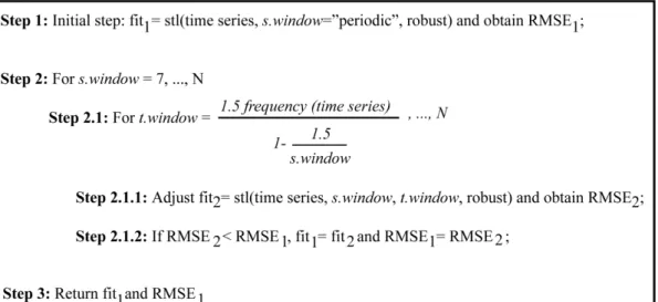
The procedure starts by setting a benchmark model, which in this case was the standard STL (Section2.3.1). Then, the error measures are determined by varying the length of the seasonal and trend window for the loess regression; finally, the best fitting model is retained. Figure2shows the steps performed for a given time series.
Remote Sens. 2016, 8, 449 6 of 16
Remote Sens. 2016, 8, 449 6 of 16
Figure 2. Schematic view of stl.fit().
The procedure was developed and implemented by the authors in the R software version 3.2.1, using the functions stl() [13] and accuracy() [42]. The inputs were the time series, the error measure (k), and whether a robust fitting was considered (robust = TRUE/FALSE). For the robust fitting, it was expected that an analysis of the data for outliers had previously been undertaken. To evaluate the best fit using RMSE, the argument k = 2 was provided; alternatively, accuracy measures, such as ME (k = 1), MAPE (k = 3) and others, were also available within the function accuracy() [42]. Therefore, the instruction is stl.fit(time series, k, robust) and, in common with the R function stl(), the output included the components (
S
t,T
t andI
t) and the smoothing parameters, but there was also an additional output for the minimum value of the chosen measure for accuracy.A seasonal plot was used to observe the inter-annual variation of the seasonal component (R function season() in forecast package [42]). The year-to-year variation of the seasonal component can be seen more clearly over time, and thus any marked changes in the seasonal pattern can be easily identified [12].
3. Results
3.1. Comparison of stl.fit() to the Standard Approach
The time series used for this comparison are a set of observations from the MERIS sensor collated as monthly means between July 2002 and March 2012 (n = 117). To examine the underlying behavior of these time series, the initial task was to search for the best model based on a measure of in-sample error, where a comparison was established between the standard stl() and the stl.fit(). Results are presented in Table 1.
The seasonal and trend loess smoothing parameters (s.window and t.window) for which the lowest RMSE was achieved are also provided (Table 1). Most of the lowest RMSE values are obtained with the lowest admissible value for the seasonal window, where s.window = 7. The choice of STL parameters determines which parts of the variation in a time series becomes either the seasonal or the trend component [11]. Therefore, smaller values for the seasonal window smoothing parameter represent a considerable variation from year to year, while larger values represent very little variation between the years [12].
Figure 2.Schematic view of stl.fit().
The procedure was developed and implemented by the authors in the R software version 3.2.1, using the functions stl() [13] and accuracy() [42]. The inputs were the time series, the error measure (k), and whether a robust fitting was considered (robust = TRUE/FALSE). For the robust fitting, it was expected that an analysis of the data for outliers had previously been undertaken. To evaluate the best fit using RMSE, the argument k = 2 was provided; alternatively, accuracy measures, such as ME (k = 1), MAPE (k = 3) and others, were also available within the function accuracy() [42]. Therefore, the instruction is stl.fit(time series, k, robust) and, in common with the R function stl(), the output included the components (St, Ttand It) and the smoothing parameters, but there was also an additional output for the minimum value of the chosen measure for accuracy.
A seasonal plot was used to observe the inter-annual variation of the seasonal component (R function season() in forecast package [42]). The year-to-year variation of the seasonal component can be seen more clearly over time, and thus any marked changes in the seasonal pattern can be easily identified [12].
3. Results
3.1. Comparison of stl.fit() to the Standard Approach
The time series used for this comparison are a set of observations from the MERIS sensor collated as monthly means between July 2002 and March 2012 (n = 117). To examine the underlying behavior of these time series, the initial task was to search for the best model based on a measure of in-sample error, where a comparison was established between the standard stl() and the stl.fit(). Results are presented in Table1.
The seasonal and trend loess smoothing parameters (s.window and t.window) for which the lowest RMSE was achieved are also provided (Table1). Most of the lowest RMSE values are obtained with the lowest admissible value for the seasonal window, where s.window = 7. The choice of STL parameters determines which parts of the variation in a time series becomes either the seasonal or the trend component [11]. Therefore, smaller values for the seasonal window smoothing parameter represent a considerable variation from year to year, while larger values represent very little variation between the years [12].
Remote Sens. 2016, 8, 449 7 of 16
Table 1. Root Mean Square Error (RMSE) comparison between stl() and stl.fit() for water leaving reflectance (ρw) between 443 and 560 nm and Algal Pigment Index 1 (API 1) (mg¨ L´1) at Stations A, B and C. The numbers in brackets (stl.fit()), are the seasonal and trend loess smoothing parameters (s.window and t.window).
A B C
stl() stl.fit() stl() stl.fit() stl() stl.fit()
ρw(443) 0.0024 0.0023 (12, 21) 0.0021 0.0019 (7, 32) 0.0019 0.0016 (7, 23)
ρw(490) 0.0023 0.0023 (116,116) 0.0018 0.0017 (7, 23) 0.0014 0.0013 (8, 26)
ρw(510) 0.0022 0.0021 (7, 23) 0.0016 0.0016 (7, 23) 0.0009 0.0009 (22, 21)
ρw(560) 0.0023 0.0022 (7, 36) 0.0017 0.0016 (7, 24) 0.0009 0.0008 (14, 36) API 1 1.3259 0.9813 (7, 26) 0.7722 0.6529 (7, 23) 0.4325 0.3900 (7, 41)
Figure3shows an example of the fitted models stl() and stl.fit() for API 1 at Station C (see also Table1), with RMSE values of 0.4325 and 0.39, respectively. Overall, the empirical results show that the fitted models provides a reasonable approximation of the original time series, particularly when using ˆYtfrom the stl.fit().
Remote Sens. 2016, 8, 449 7 of 16
Table 1. Root Mean Square Error (RMSE) comparison between stl() and stl.fit() for water leaving
reflectance (ρw)between 443 and 560 nm and Algal Pigment Index 1 (API 1) (mg·L−1) at Stations A, B
and C. The numbers in brackets (stl.fit()), are the seasonal and trend loess smoothing parameters (s.window and t.window).
A B C
stl() stl.fit() stl() stl.fit() stl() stl.fit()
ρw(443) 0.0024 0.0023 (12, 21) 0.0021 0.0019 (7, 32) 0.0019 0.0016 (7, 23)
ρw(490) 0.0023 0.0023 (116,116) 0.0018 0.0017 (7, 23) 0.0014 0.0013 (8, 26)
ρw(510) 0.0022 0.0021 (7, 23) 0.0016 0.0016 (7,23) 0.0009 0.0009 (22, 21)
ρw(560) 0.0023 0.0022 (7, 36) 0.0017 0.0016 (7, 24) 0.0009 0.0008 (14, 36)
API 1 1.3259 0.9813 (7, 26) 0.7722 0.6529 (7, 23) 0.4325 0.3900 (7, 41)
Figure 3 shows an example of the fitted models stl() and stl.fit() for API 1 at Station C (see also Table 1), with RMSE values of 0.4325 and 0.39, respectively. Overall, the empirical results show that the fitted models provides a reasonable approximation of the original time series, particularly when using Yˆt from the stl.fit().
Figure 3. Time series plot of the Algal Pigment Index 1 (API 1) and the fitted models, at Station C. 3.2. Analysis of the Decomposition of a MERIS Time Series
Decomposition plots have been used to help visualize the decomposition procedures, stl() and stl.fit(). Figure 4 displays the decomposition plot for the API 1 time series at Station C, with the original time series, in the top panel, and the seasonal, the trend and the irregular components in the lower panels.
Figure 4. Decomposition plot of API 1 for Station C using: (a) stl() (grey); and (b) stl.fit() (blue).
Figure 3.Time series plot of the Algal Pigment Index 1 (API 1) and the fitted models, at Station C. 3.2. Analysis of the Decomposition of a MERIS Time Series
Decomposition plots have been used to help visualize the decomposition procedures, stl() and stl.fit(). Figure4displays the decomposition plot for the API 1 time series at Station C, with the original time series, in the top panel, and the seasonal, the trend and the irregular components in the lower panels.
Remote Sens. 2016, 8, 449 7 of 16
Table 1. Root Mean Square Error (RMSE) comparison between stl() and stl.fit() for water leaving
reflectance (ρw)between 443 and 560 nm and Algal Pigment Index 1 (API 1) (mg·L−1) at Stations A, B
and C. The numbers in brackets (stl.fit()), are the seasonal and trend loess smoothing parameters (s.window and t.window).
A B C
stl() stl.fit() stl() stl.fit() stl() stl.fit()
ρw(443) 0.0024 0.0023 (12, 21) 0.0021 0.0019 (7, 32) 0.0019 0.0016 (7, 23)
ρw(490) 0.0023 0.0023 (116,116) 0.0018 0.0017 (7, 23) 0.0014 0.0013 (8, 26)
ρw(510) 0.0022 0.0021 (7, 23) 0.0016 0.0016 (7,23) 0.0009 0.0009 (22, 21)
ρw(560) 0.0023 0.0022 (7, 36) 0.0017 0.0016 (7, 24) 0.0009 0.0008 (14, 36)
API 1 1.3259 0.9813 (7, 26) 0.7722 0.6529 (7, 23) 0.4325 0.3900 (7, 41)
Figure 3 shows an example of the fitted models stl() and stl.fit() for API 1 at Station C (see also Table 1), with RMSE values of 0.4325 and 0.39, respectively. Overall, the empirical results show that the fitted models provides a reasonable approximation of the original time series, particularly when using Yˆt from the stl.fit().
Figure 3. Time series plot of the Algal Pigment Index 1 (API 1) and the fitted models, at Station C. 3.2. Analysis of the Decomposition of a MERIS Time Series
Decomposition plots have been used to help visualize the decomposition procedures, stl() and stl.fit(). Figure 4 displays the decomposition plot for the API 1 time series at Station C, with the original time series, in the top panel, and the seasonal, the trend and the irregular components in the lower panels.
Figure 4. Decomposition plot of API 1 for Station C using: (a) stl() (grey); and (b) stl.fit() (blue).
Remote Sens. 2016, 8, 449 8 of 16
With the standard approach (Figure4a), the seasonal amplitude and variations are constant over time, showing a fixed annual cycle. In general, the trend component is monotone decreasing along the time horizon. With stl.fit() (Figure4b), the seasonal amplitude progressively decreases until 2009, and then shows a tendency to increase for the remaining period. The trend decreases abruptly until 2006, and then is relatively constant for the remaining time period. As expected from the previous results, the irregular component has less variability (due to better fit) when compared with Figure4a.
Bars to the right side of each plot in Figure4can be used for comparisons as they represent the relative scales of the components. The bars have the same length, but have relatively different sizes as they are plotted on different scales. The long bars in the trend plots indicate that this time series exhibits a small trend, whilst the shorter bar in the seasonal plot of Figure4b compared to that in Figure4a suggests that stl.fit() is giving much more prominence to the seasonality signal than stl().
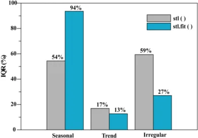
Another way of analyzing the time series decomposition is to use the interquartile range (IQR). After isolating the components, the decomposition summary identifies which component is contributing the most to the observed changes over the time series. This is deduced from the percentage of data represented within the IQR for each component, which is computed from the IQR for each component relative to the IQR of the original time series. The IQR for the data from Figure4 is presented in Figure5. Regarding the decomposition with stl(), the irregular component represent 59% of the variation, meaning that a significant percentage of the data is not captured by the model. On the other hand, the model obtained by stl.fit() shows a substantial decrease to 27% in the irregular component, as well as an increase to 94%, from 54% for stl() in the seasonal component; these difference suggest that the changes in the API 1 time series are well captured by the stl.fit() model.
Remote Sens. 2016, 8, 449 8 of 16
With the standard approach (Figure 4a), the seasonal amplitude and variations are constant over time, showing a fixed annual cycle. In general, the trend component is monotone decreasing along the time horizon. With stl.fit() (Figure 4b), the seasonal amplitude progressively decreases until 2009, and then shows a tendency to increase for the remaining period. The trend decreases abruptly until 2006, and then is relatively constant for the remaining time period. As expected from the previous results, the irregular component has less variability (due to better fit) when compared with Figure 4a.
Bars to the right side of each plot in Figure 4 can be used for comparisons as they represent the relative scales of the components. The bars have the same length, but have relatively different sizes as they are plotted on different scales. The long bars in the trend plots indicate that this time series exhibits a small trend, whilst the shorter bar in the seasonal plot of Figure 4b compared to that in Figure 4a suggests that stl.fit() is giving much more prominence to the seasonality signal than stl().
Another way of analyzing the time series decomposition is to use the interquartile range (IQR). After isolating the components, the decomposition summary identifies which component is contributing the most to the observed changes over the time series. This is deduced from the percentage of data represented within the IQR for each component, which is computed from the IQR for each component relative to the IQR of the original time series. The IQR for the data from Figure 4 is presented in Figure 5. Regarding the decomposition with stl(), the irregular component represent 59% of the variation, meaning that a significant percentage of the data is not captured by the model. On the other hand, the model obtained by stl.fit() shows a substantial decrease to 27% in the irregular component, as well as an increase to 94%, from 54% for stl() in the seasonal component; these difference suggest that the changes in the API 1 time series are well captured by the stl.fit() model.
Figure 5. Comparison of the interquartile range (IQR) for the time series in Figure 4a,b.
3.3. Modelling with stl.fit()
Figures 6 and 7 show the decomposition plots of the stl.fit() procedure for the monthly time series MERIS ρw(λ) and the MERIS water constituent API 1 at Stations A, B and C. In general, the
decomposition of the time series for all the MERIS products do not show marked differences between the three Stations, although Station A, which is closest to the coast, does have higher variability in comparison with the two Stations further offshore. The seasonal and the irregular components have the greatest influence on the time series. For all three stations, the amplitude of the seasonal term of the API 1 (Figure 7) decreases over the time period but then increases slightly towards the end. The trend component is relatively consistent for ρw(λ) (Figure 6), but for API 1
(Figure 7) a decrease is observed between July 2002 and March 2004 at the three stations, with the greater variability occurring for Station A.
Figure 5.Comparison of the interquartile range (IQR) for the time series in Figure4a,b. 3.3. Modelling with stl.fit()
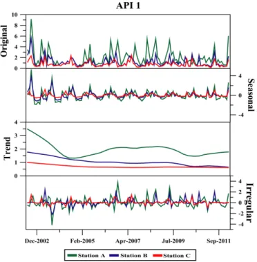
Figures6and7show the decomposition plots of the stl.fit() procedure for the monthly time series MERIS ρw(λ) and the MERIS water constituent API 1 at Stations A, B and C. In general, the decomposition of the time series for all the MERIS products do not show marked differences between the three Stations, although Station A, which is closest to the coast, does have higher variability in comparison with the two Stations further offshore. The seasonal and the irregular components have the greatest influence on the time series. For all three stations, the amplitude of the seasonal term of the API 1 (Figure7) decreases over the time period but then increases slightly towards the end. The trend component is relatively consistent for ρw(λ) (Figure6), but for API 1 (Figure7) a decrease is observed between July 2002 and March 2004 at the three stations, with the greater variability occurring for Station A.
Remote Sens. 2016, 8, 449 9 of 16
Remote Sens. 2016, 8, x 9 of 16
Figure 6. Decomposition plots of MERIS water leaving reflectance (ρw) at: (a) 443; (b) 490; (c) 510; and
(d) 560 nm, at the three Stations by stl.fit().
In terms of IQR, Table 2 shows the relative contribution of the components for the MERIS time series, in Figures 6 and 7. In general, the seasonal component dominates or is a large component of the data for all three stations. In other cases, the variation attributed to the trend is smaller than the (irregular) stochastic component, suggesting that these data do not exhibit a trend. Station A shows a high seasonality at all wavelengths with the lowest value at 510 nm (59%), and the highest value at 490 nm (75%), whilst the irregular component dominates API 1. Station B shows a high seasonality for ρw at 560 nm and a high irregular component for ρw between 443 and 510 nm, whilst the seasonal
component (75%) dominates API 1. The furthest offshore station, Station C, has ρw dominated by
seasonality at 443 and 560 nm and by the irregular component at 490 and 510 nm, where the 510 nm waveband has the highest IQR (91%). As in Station B, API 1 is dominated by the seasonal component, and this is also the station where this component has higher IQR (94%).
Figure 6.Decomposition plots of MERIS water leaving reflectance (ρw) at: (a) 443; (b) 490; (c) 510; and (d) 560 nm, at the three Stations by stl.fit().
In terms of IQR, Table2shows the relative contribution of the components for the MERIS time series, in Figures6and7. In general, the seasonal component dominates or is a large component of the data for all three stations. In other cases, the variation attributed to the trend is smaller than the (irregular) stochastic component, suggesting that these data do not exhibit a trend. Station A shows a high seasonality at all wavelengths with the lowest value at 510 nm (59%), and the highest value at 490 nm (75%), whilst the irregular component dominates API 1. Station B shows a high seasonality for ρwat 560 nm and a high irregular component for ρwbetween 443 and 510 nm, whilst the seasonal component (75%) dominates API 1. The furthest offshore station, Station C, has ρw dominated by seasonality at 443 and 560 nm and by the irregular component at 490 and 510 nm, where the 510 nm waveband has the highest IQR (91%). As in Station B, API 1 is dominated by the seasonal component, and this is also the station where this component has higher IQR (94%).
Remote Sens. 2016, 8, 449 10 of 16
Remote Sens. 2016, 8, 449 10 of 16
Figure 7. Decomposition plots of MERIS water constituent API 1 at the three Stations by stl.fit(). Table 2. Percentage of data represented within the interquartile range (IQR) for the time series components for the MERIS products water leaving reflectance (ρw) at 443, 490, 510 and 560 nm and
for the Algal Pigment Index 1 (API 1) at Stations A, B and C (dominant components are highlighted in bold).
A B C
Seasonal Trend Irregular Seasonal Trend Irregular Seasonal Trend Irregular
ρw (443) 62.9 26.9 52.4 47.1 39.9 58.1 67.9 35.9 51.2
ρw (490) 75.2 10.3 59.6 62.1 39.8 77.1 56.8 20.5 73.8
ρw (510) 59.0 27.1 45.7 55.3 35.6 73.0 65.6 27.9 90.6
ρw (560) 68.1 30.2 60.4 63.8 20.7 59.2 59.1 28.2 40.0
API 1 75.1 33.9 76.1 75.3 27.0 19.6 93.6 12.7 27.1
3.4. Inter-Annual Variability of the Seasonal Component of MERIS API 1
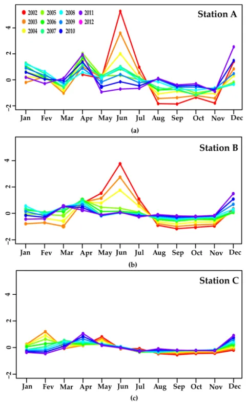
Figure 8 shows the inter-annual variability of the MERIS API 1 where the seasonal component is compared for different years of the time series. The inter-annual variability between years decreases from Station A to Station C. The higher variability at Station A (Figure 8a) occurs in the months of June followed by December and then between the spring months of March and April. Station B (Figure 8b) also has a similar pattern to Station A, but less pronounced. The most offshore Station C (Figure 8c) shows only small changes over the year, with an inter-annual variability that is less than the other Stations. In common with Stations A and B, Station C show some variability in December and April months, but in contrast to the other stations, Station C also show variability in February and in May, particularly, during the first three years of the time series.
Figure 7.Decomposition plots of MERIS water constituent API 1 at the three Stations by stl.fit(). Table 2. Percentage of data represented within the interquartile range (IQR) for the time series components for the MERIS products water leaving reflectance (ρw) at 443, 490, 510 and 560 nm and for the Algal Pigment Index 1 (API 1) at Stations A, B and C (dominant components are highlighted in bold).
A B C
Seasonal Trend Irregular Seasonal Trend Irregular Seasonal Trend Irregular
ρw(443) 62.9 26.9 52.4 47.1 39.9 58.1 67.9 35.9 51.2
ρw(490) 75.2 10.3 59.6 62.1 39.8 77.1 56.8 20.5 73.8
ρw(510) 59.0 27.1 45.7 55.3 35.6 73.0 65.6 27.9 90.6
ρw(560) 68.1 30.2 60.4 63.8 20.7 59.2 59.1 28.2 40.0
API 1 75.1 33.9 76.1 75.3 27.0 19.6 93.6 12.7 27.1
3.4. Inter-Annual Variability of the Seasonal Component of MERIS API 1
Figure8shows the inter-annual variability of the MERIS API 1 where the seasonal component is compared for different years of the time series. The inter-annual variability between years decreases from Station A to Station C. The higher variability at Station A (Figure8a) occurs in the months of June followed by December and then between the spring months of March and April. Station B (Figure8b) also has a similar pattern to Station A, but less pronounced. The most offshore Station C (Figure8c) shows only small changes over the year, with an inter-annual variability that is less than the other Stations. In common with Stations A and B, Station C show some variability in December and April months, but in contrast to the other stations, Station C also show variability in February and in May, particularly, during the first three years of the time series.
Remote Sens. 2016, 8, 449 11 of 16
Remote Sens. 2016, 8, 449 11 of 16
Figure 8. Inter-annual variability of the seasonal component of the MERIS water constituent Algal Pigment Index 1 (API 1) at: (a) Station A; (b) Station B; and (c) Station C. Each line represents a year from 2002 to 2012.
4. Discussion
Ocean color remote sensing data can provide a temporal and spatial view of the phytoplankton biomass distribution for long data series. However, there is also a need to develop quantitative methods for identifying and interpreting the fluctuations in the biomass distribution over the duration of the time series [45]. The present study at Sagres has developed the stl.fit() as a tool to provide an analysis of ocean color time series data from this region, to identify the historical changes over time and to provide a richer diagnosis and clearer interpretation of the temporal variability and its potential causes. The study has focused on the inter-annual variation of the changes of the phytoplankton to better understand the dynamics of the coastal waters off Sagres.
Figure 8.Inter-annual variability of the seasonal component of the MERIS water constituent Algal Pigment Index 1 (API 1) at: (a) Station A; (b) Station B; and (c) Station C. Each line represents a year from 2002 to 2012.
4. Discussion
Ocean color remote sensing data can provide a temporal and spatial view of the phytoplankton biomass distribution for long data series. However, there is also a need to develop quantitative methods for identifying and interpreting the fluctuations in the biomass distribution over the duration of the time series [45]. The present study at Sagres has developed the stl.fit() as a tool to provide an analysis of ocean color time series data from this region, to identify the historical changes over time and to provide a richer diagnosis and clearer interpretation of the temporal variability and its potential
Remote Sens. 2016, 8, 449 12 of 16
causes. The study has focused on the inter-annual variation of the changes of the phytoplankton to better understand the dynamics of the coastal waters off Sagres.
4.1. The stl.fit() Approach
The characterization the changes that occur in the Sagres region is based on the STL decomposition method proposed by Cleveland et al. [11], but instead of considering the standard stl(), where the seasonal smoothing parameter is assumed to be periodic, stl.fit() has been developed to obtain “automatically” the seasonal and trend smoothing parameters by minimizing an error measure that enables optimal modeling of the data. This approach is an iterative computational estimate of the seasonal and trend components, where the trend component is obtained using the non-parametric loess regression and the seasonality from the trend adjusted series.
Another feature that is considered by STL is its robustness to extreme and other aberrant observations. There are studies (e.g., Vantrepotte and Mélin [3], Vantrepotte and Mélin [4], Vantrepotte and Mélin (2009) [46], and Volpe et al. (2012) [10]) that remove these observations from the data, whereas STL solve this situation without reducing the dataset. Moreover, an analysis has been performed that detects the dominant components in the time series, using a statistical dispersion measure that is not influenced by outliers. Thus, the empirical results based on an error measure indicates that the best model is achieved using the stl.fit(), instead of the standard approach. This is important because the initial objective of the study was to obtain a statistical model that can better describe the stochastic behavior of a time series, enabling a statistical analysis that will improve the diagnosis and interpretation of the changes in the ocean color products retrieved by the satellite data. In summary, stl.fit() is capable of capturing the variations in the seasonal dynamics and takes advantage of the useful features of the STL time series decomposition method. Nevertheless, stl.fit() also inherits the disadvantages of STL, i.e., that it does not handle calendar variations and only considers an additive decomposition [12].
4.2. MERIS Time Series
Using around 10 years of MERIS ρw(λ) and API 1 products, this study has evaluated the performance of stl.fit() for the decomposition of time series for ocean color satellite data. The decomposition (Figures6and7) shows that the data can be split into seasonal, trend and irregular components. The decomposition has detected the strength of the time series components, which were deduced from the percentage of data represented within the IQR. Station A shows a seasonal dominance for all the reflectance wavebands, which is a similar finding to that observed by Vantrepotte and Mélin [3] for the normalized water leaving radiances from SeaWiFS for the Iberian area. For the other two stations, the model is not capable of modeling the trend and the seasonality, probably due to the high variability in the data.
When the seasonal components of the ρw(at 443, 490, 510 and 560 nm) and the API 1 product are compared, a relationship is observed between them, as might be expected as the visible wavelengths of ρw(λ) are part of the API 1 algorithm. However, in Figure6d, the seasonal effect is less variable (for 510 and 560 nm) and seems to decrease over time (for 560 nm) compared to 443 and 490 nm. The lower variability in the green bands is probably because the reflectance is not strongly influenced by the absorption of phytoplankton, which is the dominant optical constituent within this region [24,25]. However, the higher seasonal variability at the start of the time series is also seen in the MERIS API 1 product, which could indicate a change in the dominant phytoplankton functional types, i.e., higher values in the green bands indicate higher scattering that could be coming from the phytoplankton. The decline in the concentration of phytoplankton (TChla, retrieved by API 1), together with the simultaneous decrease in seasonal amplitude, is consistent with the findings of Vantrepotte and Mélin [4] for the Northeast Atlantic area.
The MERIS API 1 product is dominated mainly by the seasonal component, with an increase in dominance as the distance increases offshore from Station A to Station C. As in Vantrepotte and
Remote Sens. 2016, 8, 449 13 of 16
Mélin [4], this site shows an inter-annual variability that is dominated by the phytoplankton seasonal variability that is linked to the physical oceanography influencing the study area. The main source of nutrients for the phytoplankton depends on the seasonal pattern of upwelling events [25,47,48]; other sources of nutrients are limited as there are no permanent rivers [29,47].
Although the difference between the seasonal and the irregular components is not significant, the dominance of the irregular component is slightly higher for the coastal Station (A). This can probably be explained by an increased failure of the atmospheric correction due to the adjacency effects from land, which are discussed in more detail in Cristina et al. [22]. Therefore, these results suggest that future studies should try processing the time series with the Improved Contrast between Ocean and Land (ICOL) processor; to reduce errors in the processing chain for sites close to land by correcting for the adjacency effects.
An example of how stl.fit() can contribute to the analysis of the MERIS time series at the Sagres site is provided be comparing plots of the inter-annual variability for the seasonal component of the MERIS API 1 at the Sagres Stations (Figure8). Essentially, these seasonal plots show the months with the highest variability at each Station. These data provide important information about periods when management action might be needed, for example, for aquaculture activities, or when in situ sampling should be implemented for monitoring purposes, e.g., to conform to EU Directives. In the case of Sagres the data shows that each Station should be sampled at least once per season, to show changes in the ecosystem. In particular Station A and B should be sampled in spring (from March and April), in summer (during June), in autumn (from September and November) and in the winter (during December). Alternatively, Station C should be sampled in spring (from March to May), in summer (from June to August), in autumn (from September to November) and in the winter (from December to February).
With regard to the two research questions presented in the Introduction Section: (1) Will stl.fit() capture the dynamics of the time series of the study area better?
Without repeating the details that have been presented already, the improvements provided by stl.fit() are clearly demonstrated in Table1and Figures3–7.
(2) How can stl.fit() be used to describe and explain the variability of the study area?
The final section of both the Results and the Discussion provide an example showing the inter-annual variability of the seasonal component of MERIS API 1 (see Figure 8). Many other examples could be provided.
5. Conclusions
‚ This study has analyzed the MERIS time series for the products, water leaving reflectance ρw(λ) and the Algal Pigment Index 1 (API 1) at Sagres on the SW coast of Iberia. The optical characteristics of this area are well characterized from in situ validation of MERIS between 2008 and 2012.
‚ The variation in the MERIS time series has been decomposed into components representing seasonal (St), trend (Tt) and irregular (It) fluctuations using the Seasonal-Trend decomposition (STL) based on Loess. The advantages of STL is that it can identify a seasonal component that changes over time, it is responsive to nonlinear trends, and it is robust in the presence of outliers. It is also available within the R software through the stl() function.
‚ One of the novelties in this study is the development of stl.fit() which has the advantages of the STL but also allows an automatic selection of the best model, by varying the values of the smoothing parameters, based on minimizing the error measure.
‚ After decomposing the MERIS products time series into seasonal, trend and irregular components, the interquartile range is taken into account. The ρw(λ) product is dominated by both the
Remote Sens. 2016, 8, 449 14 of 16
seasonal and irregular components, whilst the API 1 product is dominated mainly by the seasonal component, with an increasing effect from inshore to offshore.
‚ The comparison of the seasonal components between the ρw(λ) and the API 1 product at Sagres site, shows that the variations during the 10 years of monthly observations decrease along this period . ‚ A more detailed study of the inter-annual seasonal variation for API 1 shows the influence of
upwelling events, and in which month(s) of the year these occur at each of the three stations at Sagres. Most of the inter-annual seasonal variability of MERIS products can be explained by the optically significant constituents of these waters. Nevertheless, future studies should also take into account the physical and climatic variables that are related to and influence the ρw(λ) and API 1 off Sagres.
‚ This study, demonstrates how stl.fit() procedure is a good option for any remote sensing study of time series, particularly those addressing inter-annual seasonal variations. This procedure will be made available in R software, so that it is accessible to a wider community, including other fields of research.
Acknowledgments: Sónia Cristina and Priscila Costa Goela are funded by PhD grants from the Portuguese FCT(SFRH/BD/78354/2011 and SFRH/BD/78356/2011, respectively); Alice Newton is funded by EU FP7 project DEVOTES (grant no. 308392); John Icely is funded by EU FP7 AQUA-USER (grant no. 607325), and Horizon 2020 AquaSpace (grant no. 633476); and Clara Cordeiro is funded by FCT-Fundação para a Ciência e Tecnologia, Portugal, through the project UID/MAT/00006/2013. We also thank ESA and ACRI-ST for access to ODESA MEGS®(http://earth.eo.esa.int/odesa). The Authors thank the four external Reviewers for their sound advice on improvements to the article.
Author Contributions: Sónia Cristina was responsible for the research design, satellite image processing, data preparation and analysis and writing the manuscript. Clara Cordeiro was responsible for the stl.fit() design and implementation in the R software, writing the manuscript and statistical interpretation guidance. Samantha Lavender contributed to the research design and manuscript editing. Priscila Goela contributed to the manuscript editing, and with scientific consultancy. John Icely and Alice Newton provided the research facilities, and contributed to editing and reviewing the manuscript.
Conflicts of Interest:The authors declare no conflict of interest. References
1. Zibordi, G.; Berthon, J.-F.; Mélin, F.; D’Alimonte, D. Cross-site consistent in situ measurements for satellite ocean color applications: The BiOMaP radiometric dataset. Remote Sens. Environ. 2011, 115, 2104–2115.
[CrossRef]
2. Kirchgässner, G.; Wolters, J.; Hassler, U. Introduction to Modern Time Series Analysis; Springer-Verlag: Berlin, Germany; Heidelberg, Germany, 2008.
3. Vantrepotte, V.; Mélin, F. Temporal variability in SeaWiFS derived apparent optical properties in European seas. Cont. Shelf Res. 2010, 30, 319–334. [CrossRef]
4. Vantrepotte, V.; Mélin, F. Inter-annual variations in the SeaWiFS global chlorophyll a concentration (1997–2007). Deep Sea Res. Part I 2011, 58, 429–441. [CrossRef]
5. Mélin, F.; Vantrepotte, V.; Clerici, M.; D’Alimonte, D.; Zibordi, G.; Berthon, J.F.; Canuti, E. Multi-sensor satellite time series of optical properties and chlorophyll-a concentration in the Adriatic Sea. Prog. Oceanogr. 2011, 91, 229–244. [CrossRef]
6. Zibordi, G.; Mélin, F.; Berthon, J.-F. Intra-annual variations of biases in remote sensing primary ocean color products at a coastal site. Remote Sens. Environ. 2012, 124, 627–636. [CrossRef]
7. Alikas, K.; Kangro, K.; Randoja, R.; Philipson, P.; Asukull, E.; Pisek, J.; Reinart, A. Satellite-based products for monitoring optically complex inland waters in support of EU Water Framework Directive. Int. J. Remote Sens. 2015, 36, 4446–4468. [CrossRef]
8. Bisgaard, S.; Kulahci, M. Time series model selection. In Book Time Series Analysis and Forecasting by Example, 1st ed.; Shewhart, W.A., Wilks, S.S., Eds.; John Wiley & Sons, Inc. Publication: Hoboken, NJ, USA, 2011; pp. 155–175.
Remote Sens. 2016, 8, 449 15 of 16
9. Loisel, H.; Mangin, A.; Vantrepotte, V.; Dessailly, D.; Dinh, D.N.; Garnesson, P.; Ouillon, S.; Lefebvre, J.-P.; Mériaux, X.; Phan, T.M. Variability of suspended particulate matter concentration in coastal waters under the Mekong’s influence from ocean color (MERIS) remote sensing over the last decade. Remote Sens. Environ. 2014, 150, 218–230.
10. Volpe, G.; Colella, S.; Forneris, V.; Tronconi, C.; Santoleri, R. The mediterranean ocean colour observing system—System development and product validation. Ocean Sci. 2012, 8, 869–883. [CrossRef]
11. Cleveland, R.B.; Cleveland, W.S.; McRae, J.E.; Terpenning, I. STL: A seasonal-trend decomposition procedure based on loess. J. Off. Stat. 1990, 6, 3–73.
12. Hyndman, R.; Athanasopoulos, G. Forecasting: Principles and Practice. Available online: http://otexts.org/ fpp/ (accessed on 8 September 2015).
13. R Core Team. R: A Language and Environment for Statistical Computing; R Foundation for Statistical Computing: Vienna, Austria, 2015.
14. Ndungu, J.; Monger, B.C.; Augustijn, D.C.; Hulscher, S.J.; Kitaka, N.; Mathooko, J.M. Evaluation of spatio-temporal variations in chlorophyll-a in Lake Naivasha, Kenya: Remote-sensing approach. Int. J. Remote Sens. 2013, 34, 8142–8155. [CrossRef]
15. Lu, H.; Li, Y.; Clilverd, M.A.; Jarvis, M.J. Trend and abrupt changes in long-term geomagnetic indices. J. Geophy. Res. Space 2012, 117, 1–14. [CrossRef]
16. Petropavlovskikh, I.; Evans, R.; McConville, G.; Manney, G.L.; Rieder, H.E. The influence of the North Atlantic Oscillation and El Niño-Southern Oscillation on mean and extreme values of column ozone over the United States. Atmos. Chem. Phys. 2015, 15, 1585–1598. [CrossRef]
17. Brown, C.W.; Uz, S.S.; Corliss, B.H. Seasonality of oceanic primary production and its interannual variability from 1998 to 2007. Deep Sea Res. Part I 2014, 90, 166–175. [CrossRef]
18. Novoa, S.; Chust, G.; Sagarminaga, Y.; Revilla, M.; Borja, A.; Franco, J. Water quality assessment using satellite-derived chlorophyll-a within the European directives, in the southeastern Bay of Biscay. Mar. Pollut. Bull. 2012, 64, 739–750. [CrossRef] [PubMed]
19. Cristina, S.; Icely, J.; Goela, P.C.; DelValls, T.A.; Newton, A. Using remote sensing as a support to the implementation of the European Marine Strategy Framework Directive in SW Portugal. Cont. Shelf Res. 2015, 108, 169–177. [CrossRef]
20. Kratzer, S.; Harvey, E.T.; Philipson, P. The use of ocean color remote sensing in integrated coastal zone management—A case study from Himmerfjärden, Sweden. Mar. Policy 2014, 43, 29–39. [CrossRef] 21. Harvey, E.T.; Kratzer, S.; Philipson, P. Satellite-based water quality monitoring for improved spatial and
temporal retrieval of chlorophyll-a in coastal waters. Remote Sens. Environ. 2015, 158, 417–430. [CrossRef] 22. Cristina, S.C.V.; Moore, G.F.; Goela, P.R.F.C.; Icely, J.D.; Newton, A. In situ validation of MERIS marine
reflectance off the southwest Iberian Peninsula: Assessment of vicarious adjustment and corrections for near-land adjacency. Int. J. Remote Sens. 2014, 35, 2347–2377.
23. Cristina, S.V.; Goela, P.; Icely, J.D.; Newton, A.; Fragoso, B. Assessment of water-leaving reflectances of oceanic and coastal waters using MERIS satellite products off the southwest coast of Portugal. J. Coast. Res. 2009, 56, 1479–1483.
24. Goela, P.C.; Icely, J.; Cristina, S.; Newton, A.; Moore, G.; Cordeiro, C. Specific absorption coefficient of phytoplankton off the southwest coast of the Iberian Peninsula: A contribution to algorithm development for ocean colour remote sensing. Cont. Shelf Res. 2013, 52, 119–132. [CrossRef]
25. Goela, P.C.; Icely, J.; Cristina, S.; Danchenko, S.; DelValls, T.; Newton, A. Using bio-optical parameters as a tool for detecting changes in the phytoplankton community (SW Portugal). Estuar. Coast. Shelf Sci. 2015, 167, 125–137. [CrossRef]
26. Goela, P.; Danchenko, S.; Icely, J.; Lubián, L.; Cristina, S.; Newton, A. Using CHEMTAX to evaluate seasonal and interannual dynamics of the phytoplankton community off the South-west Coast of Portugal. Estuar. Coast. Shelf Sci. 2014, 151, 112–123. [CrossRef]
27. Goela, P.; Newton, A.; Cristina, S.; Fragoso, B. Water framework directive implementation: Intercalibration exercise for biological quality elements—A case study for the south coast of Portugal. J. Coast. Res. 2009, 56, 1214–1218.
28. Loureiro, S.; Icely, J.; Newton, A. Enrichment experiments and primary production at Sagres (SW Portugal). J. Exp. Mar. Biol. Ecol. 2008, 359, 118–125. [CrossRef]
Remote Sens. 2016, 8, 449 16 of 16
29. Loureiro, S.; Reñé, A.; Garcés, E.; Camp, J.; Vaqué, D. Harmful algal blooms (HABs), dissolved organic matter (DOM), and planktonic microbial community dynamics at a near-shore and a harbour station influenced by upwelling (SW Iberian Peninsula). J. Sea Res. 2011, 65, 401–413. [CrossRef]
30. Relvas, P.; Barton, E.D. Mesoscale patterns in the Cape São Vicente (Iberian Peninsula) upwelling region. J. Geophys. Res. Oceans 2002, 107, 28:1–28:23. [CrossRef]
31. Loureiro, S.; Newton, A.; Icely, J.D. Microplankton composition, production and upwelling dynamics in Sagres (SW Portugal) during the summer of 2001. Sci. Mar. 2005, 69, 323–341.
32. Ramos, A.M.; Pires, A.C.; Sousa, P.M.; Trigo, R.M. The use of circulation weather types to predict upwelling activity along the western Iberian Peninsula coast. Cont. Shelf Res. 2013, 69, 38–51. [CrossRef]
33. Basic ERS & ENVISAT (A) ATSR and MERIS Toolbox (BEAM Version 4.11). Available online: http://www. brockmann-consult.de/cms/web/beam/ (accessed on 1 September 2015).
34. Optical Data Processor of the European Space Agency (ODESA). Available online: http://www.odesa-info. eu/process_basic/basic.php (accessed on 1 September 2015).
35. MERIS Quality Working Group (QWG). MERIS 3rd Data Reprocessing—Software and ADF Updated, Technical Document Ref. A879.NT.008.ACRI-ST. 27 June 2011. Available online: https://earth.esa.int/web/ guest/-/meris-3rd-data-reprocessing-software-and-adf-updates-7929 (accessed on 30 September 2015). 36. Morel, A.; Antoine, D. Pigment Index Retrieval in Case 1 Waters, Algorithm Theoretical Basis Document
PO-TN-MEL-GS-0005. 2007. Available online: https://earth.esa.int/documents/700255/2042855/MERIS_ ATBD_2.9_v4.3+-+2011.pdf (accessed on 30 September 2015).
37. Morel, A.; Huot, Y.; Gentili, B.; Werdell, P.J.; Hooker, S.B.; Franz, B.A. Examining the consistency of products derived from various ocean color sensors in open ocean (Case 1) waters in the perspective of a multi-sensor approach. Remote Sens. Environ. 2007, 111, 69–88. [CrossRef]
38. Brockmann, C. Limitations of the application of the MERIS atmospheric correction. In Proceedings of the Second Working Meeting on MERIS and AATSR Calibration and Geophysical Validation, Frascati, Italy, 20–24 March 2006.
39. ESA. MERIS Product Handbook Issue 3.0. Available online: https://earth.esa.int/handbooks/meris/CNTR. html (accessed on 7 September 2015).
40. Steinmetz, F.; Deschamps, P.Y.; Ramon, D. Atmospheric correction in presence of sun glint: Application to MERIS. Opt. Express 2011, 19, 9783–9800. [CrossRef] [PubMed]
41. Smith, M.E.; Bernard, S.; O’Donoghue, S. The assessment of optimal MERIS ocean colour products in the shelf waters of the KwaZulu-Natal Bight, South Africa. Remote Sens. Environ. 2013, 137, 124–138. [CrossRef] 42. Hyndman, R.J. Forecast: Forecasting Functions for Time Series and Linear Models, R Package Version 6.2.
Available online: http://github.com/robjhyndman/forecast (accessed on 30 October 2015).
43. Qian, S.S.; Borsuk, M.E.; Stow, C.A. Seasonal and long-term nutrient trend decomposition along a spatial gradient in the Neuse River watershed. Environ. Sci. Technol. 2000, 34, 4474–4482. [CrossRef]
44. Jiang, B.; Liang, S.; Wang, J.; Xiao, Z. Modeling MODIS LAI time series using three statistical methods. Remote Sens. Environ. 2010, 114, 1432–1444. [CrossRef]
45. Pezzulli, S.; Stephenson, D.B.; Hannachi, A. The variability of seasonality. J. Clim. 2005, 18, 71–88. [CrossRef] 46. Vantrepotte, V.; Mélin, F. Temporal variability of 10-year global SeaWiFS time-series of phytoplankton
chlorophyll-a concentration. ICES J. Mar. Sci. 2009, 66, 1547–1556. [CrossRef]
47. Cardeira, S.; Rita, F.; Relvas, P.; Cravo, A. Chlorophyll a and chemical signatures during an upwelling event off the South Portuguese coast (SW Iberia). Cont. Shelf Res. 2013, 52, 149. [CrossRef]
48. Goela, P.C.; Cordeiro, C.; Danchenko, S.; Icely Cristina, S.; Newton, A. Time series analysis of data for Sea Surface Temperature and Upwelling components from the Southwest Coast of Portugal. J. Mar. Syst. 2016, under review.
© 2016 by the authors; licensee MDPI, Basel, Switzerland. This article is an open access article distributed under the terms and conditions of the Creative Commons Attribution (CC-BY) license (http://creativecommons.org/licenses/by/4.0/).