PRODUCTIVE EFFICIENCY OF PORTUGUESE VINEYARD REGIONS
Ana MARTA-COSTA
Corresponding author. Assistant Professor. University of Trás-os-Montes e Alto Douro (UTAD) and Centre for Transdisciplinary Development Studies (CETRAD), Portugal, www.utad.pt
amarta@utad.pt Vítor MARTINHO
Coordinator Professor. Agricultura School, Polytechnic Institute of Viseu, Portugal vdmartinho@esav.ipv.pt.
Micael SANTOS
Research fellow. University of Trás-os-Montes e Alto Douro (UTAD) and Centre for Transdisciplinary Development Studies (CETRAD)
micaels@utad.pt Abstract
The overall globalization in wine industry and the search for sustainability of the sector has increased competition which highlights the importance of productivity gains. The purpose of this paper is to analyse the productive efficiency of the viticulture sector for the Portuguese regions, over the period 1989 to 2007, with data from the EUFADN, using both a deterministic and stochastic approach. The results show an increase of Technical Efficiency (TE) when used the stochastic frontiers analysis (SFA) in all regions, while the data envelopment analysis (DEA) approach through the Malmquist index reveals a stabilization of TE.
Keywords: Efficiency, productivity, Portuguese regions, viticulture. JEL classification: C6, Q1
1. Introduction
Over the last decades the wine industry has been subject to an intensive globalization and international competition, a fact that poses both challenges and opportunities to the wine regions, which are compelled to adopt innovative strategies.
Despite recent impressive performance of the New World wine countries, both in output and exports, the European Union (EU-28) continues to be, in 2014, world’s leader in wine production, occupying almost 50% of vineyards area worldwide and responsible for around 65% of the wine production by volume and trade (GAIN, 2015). Nevertheless, the recent trend has been for the EU-28 vine growing area (of just under 3.5 million ha in 2013) to decline, due to shrinking margins and EU subsidies paid to farmers to uproot their vines. The EU’s Common Agriculture Policy (CAP) aims to increase the competitiveness of the wine industry, maintaining the best traditional practices, reinforcing the rural social fabric and preserving environmental sustainability.
The winemaking sector plays also a key role in the Portuguese economy. Portugal is the 11th wine producer and the 9th exporter in value and volume in the world (OIV, 2016). Half of the total national wine production is exported, which represents nearly 2% of national exports (IVV, 2013). Portugal’s 2014 wine production was 3.62% of the EU-28 (589 million litres) and the 2015 grape growing area was 217,000 ha (GAIN, 2015 and OIV, 2016). The country is divided into 14 main high quality wine producing region.
In recent decades the grapevine/wine sector has been modernized, creating strict regulations to guarantee wine characteristics, making this sector generally more competitive on the global market. However, the increase of competitiveness imposed by globalization has led new challenges and threats for the survival of the firms in the wine sector (Sellers-Rubio et al., 2016). The grape growers should achieve better levels of efficiency and improve the performance of their firms who makes the studies on the productive efficiency more important. The producers always aspire at increasing the efficiency of their production process, but they do not always succeed in optimizing it. The research of reasons behind firm
inefficiency is very important to correct fragilities and to improve efficiency in the production context.
The production efficiency estimation regarding different vineyard systems plays an important role in the field of economic context, as it allows managements to reach high levels of performance restricting resources, minimizing undesired inputs or optimizing desired outputs. However, organizations’ competitiveness allied to efficiency analysis must be allocated also as a key tool in improving social wellbeing and promoting sustainable development (Marta-Costa, 2010a, 2010b; Marta-Costa and Silva, 2013) as the concept evolves the parsimony use of economic resources in order to reach cost minimization, output and profit maximization (Sampaio, 2013). Given the continuous pressure on vineyard products’ margins, improvements in organisations’ economic efficiency can boost the financial situation of both farms and vineyard-dependent communities.
The aim of this paper is to analyse the Technical Efficiency (TE) of the vineyard sector in Portuguese regions, using both a deterministic and stochastic approach, over the period 1989 to 2007, using data from the European Farm Accountancy Data Network (EUFADN, 2017). 2. Productive Efficiency of Viticulture Sector: A Literature Review
The concept of productive efficiency has been decomposed into technical and allocative efficiency, by Farrel (1957). The first occurs when given a certain level of inputs, the Decision Making Unit (DMU) is able to produce the maximum level of outputs or, given a certain level of output, the DMU is able to minimize the level of input (Fleming et al., 2014). The allocative efficiency reflects the ability of a firm to use the inputs in optimal proportions, given their respective prices to minimize the cost or maximize the revenue (Aparicio et al., 2013).
Increasing production efficiency on the wine sector calls for a better understanding of the key factors driving the performance of vineyard systems. This could be a difficult task due to the heterogeneous characteristics of the used production systems (Sellers-Rubio et al., 2016). For instance, in the case of Portugal, the farms are composed by several blocks and each block represent a different variety of grapes/vines and management. The multiple effects of the grapevine physiology and the grapevine-environment-agronomy interactions are widely recognised, and have implications on yield and berry quality, which in turn determine the major drivers of the vineyard efficiency.
Related to the heterogeneous characteristics of the used production systems, for example Moreira et al. (2011), in their study of Chilean wine grape producers, classified four categories of planting vine systems: simple cordon, double cordon, pergola and other training system, which affect the productive efficiency of farms. The pergola system was the most productive, while the simple and double cordon were less productive. Regarding to TE the other training systems exhibit a highest level, followed by simple cordon, pergola and double cordon.
Other studies relate efficiency levels both to microeconomic factors, such as farm and farmer characteristics (Conradie et al., 2006; Henriques et al., 2009); grape variety (Coelli and Sanders, 2013; Manevska-Tasevska, 2013); diversification and specialisation (Henriques et al., 2009; Coelli and Sanders, 2013); irrigation (Conradie et al., 2006; Henriques et al., 2009), and to macroeconomic factors, such as developments in the financial system; the quality of human capital, and per capita wine consumption (József and Péter, 2014).
The value and volume of grapes or wine are the main variables identified by the literature regarding the outputs of the vineyard systems. According to Sellers-Rubio et al. (2016) and Sellers-Rubio and Más-Ruiz (2015) the output in monetary terms reveals the ability of wine producer to transform inputs into wine outputs value or value of grapes produced and it represents the economic concept of efficiency. Although the quantity of output in volume corresponds to the technical concept of efficiency and it is evaluated by the wine producer ability to transform some inputs into litres of wine or quantity of grapes produced.
In other words, some farms are concerned to produce as much as possible at the lowest price, while other prefers to produce less and with higher quality to sell wines with a higher price. According to Coelli and Sanders (2013) variable of output estimated in quantity terms does not take into account differences in quality. The production efficiency estimation of wine sector, in terms of quantity, is present in the studies of Tóth & Gál (2014), Moreira et al.
(2011) and Freitas (2014). Although, the production efficiency estimation, in terms of value, giving attention not only to price of each wine or grape produced but also to the quantity, was developed by Sellers-Rubio et al. (2016), Sellers-Rubio & Más-Ruiz (2015), Aparicio et al. (2013), Vidal et al. (2013), Brandano et al (2012), and Henriques et al. (2009).
These two ways of efficiency conceptualizations of the farms is of great importance in supporting famers’ decisions to adapt their vineyards and production systems and open discussion regarding the model to pursue for the future, sometimes associated with the availability of the data.
The studies with values of output use variables such us sales revenue, profit volume and earnings (Sellers-Rubio et al. 2016; Sellers-Rubio & Máz-Ruiz, 2015; and Brandano et al., 2012), total output in value (Henriques et al., 2009) and value of domestic and foreign sales (Aparicio et al., 2013; Vidal et al., 2013). While when output are in volume the used variables are the quantity of wine production (Tóth & Gál, 2014) and quantity of grapes produced (Moreira et al., 2011; Freitas, 2014).
For inputs, we found three main categories of variables for the study of the vine-growing system efficiency: labour, capital and land. However, intermediate consumption can be an important input like Freitas (2014) studied. Moreover, Coelli and Sanders (2013) identify irrigation for inputs too, but this variable is important only for dryland farms. Some studies identify only two inputs (labour and capital), such as Rubio et al. (2016), Sellers-Rubio & Más-Ruiz (2015), Freitas (2014) and Brandano et al. (2012). But, Tóth & Gál (2014), Moreira et al. (2011) and Henriques et al. (2009) added the used land while Aparicio et al. (2013) used also the number of vinegrowers. Other studies (Aparicio et al., 2013; Vidal et al., 2013) opted by the lonely input of land.
Also, the same variable could be measured by different ways. The labour input is studied by the number of employees (Sellers-Rubio et al., 2016; Sellers-Rubio & Más-Ruiz, 2015) or by agricultural employment (Tóth & Gál, 2014), labour cost (Moreira et al., 2011; Brandano et al., 2012) or by work hours (Freitas, 2014; Henriques et al., 2009). The land input variable seems to be more consensual and are measured by the used area of land in hectares. For the capital input, the papers use some variables such as equity level of winery (Sellers-Rubio et al., 2016), funds of company (Sellers-Rubio & Más-Ruiz, 2015), level of debt (Sellers-Rubio et al., 2016; Sellers-Rubio et al., 2015), net agricultural capital stock (Tóth & Gál, 2014) and capital like machinery costs and other fixed assets (Moreira et al., 2011; Freitas, 2014; Brandano et al. 2012; and Henriques et al., 2009). In addition to these inputs, some studies also include the intermediate consumption with the vegetal production such the costs with pesticides and fertilizers (Moreira et al. 2011; Freitas, 2014; and Henriques et al., 2009).
These multiplicity of the variables used for productive efficiency estimation intensifies the discussion about the different results that could be gathered and how could they influence the decision of the farmers and other stakeholders of the industry. Besides the main groups of variables of outputs and inputs, the literature refers also to other variables regarding the inefficiency of the farms. Some examples of these variables are the access to finance, planting vine system, type of wine, grape quality, type of firm, employment rate, average of wages paid, gross domestic product and others (Moreira et al., 2011; Fuensantana et al., 2015; Tóth & Gal, 2014).
In general, the reflection of the literature of production efficiency studies shows that there are some variables that are consensual and common in several works, as land area, labour and capital (inputs). However, there are other variables that can affect the efficiency in different ways but there are not consensual. The great diversity of variables that have already been used, makes the study of productivity and efficiency very complex and complicated to estimate. Despite this, these studies are very important for wine-growing producers because the efficiency is a goal that they have in mind.
Empirical studies have adopted two main alternative approaches, often based either on (non-parametric, non-stochastic) mathematical programming models or on (stochastic, parametric) econometric models. Both are very useful to support decision-making because they give an indication of what the main characteristics of farm are and how some of the problems identified may be solved (Silva et al., 2013).
According to Coelli et al. (2005) exist four methods: least-squares econometric production models; total factor productivity indices; data envelopment analysis (DEA); and stochastic
frontiers analysis (SFA). The first two models assume that all firms are technically efficient, although the last two are the methods most used to estimate efficiency especially at one point in time. While the method least-squares econometric production models and stochastic frontiers involve the econometric estimation of parametric functions, the method total factor productivity indices and DEA do not (Coelli et al, 2005).
The DEA and SFA are the methods most used in literature of productive efficiency. DEA estimate the efficiency frontier and the distance of production frontier of the DMUs to the efficient frontier give us a measure of inefficient (Sellers-Rubio et al., 2016; Sellers-Rubio & Más Ruiz, 2015; Brandano et al., 2012). DEA is a non-parametric methodology based on linear programing techniques and is not necessary to include specific functional forms for the production function (relationship between inputs and outputs) to establish the efficient frontier (Sellerrs-Rubio & Más Ruiz, 2015; Brandano et al., 2012; Cullinane et al., 2006; Henriques et al., 2009; Moreira et al., 2011). A DMU is efficient in DEA analysis if no other DMU is able to produce more outputs from the same inputs or is able to produce the same outputs with less inputs (Sellers-Rubio & Más Ruiz, 2015). Moreover, a DEA can study a framework with multiple input-output focuses on a virtual single input-output structure (Brandano et al., 2012; Cullinane et al., 2006). Furthermore, DEA considers specification error as minimal, so not consider random shocks or measurement errors and all factor are due to inefficiency (Cullinane et al., 2006). When panel data is available, the DEA allows the calculation of the Malmquist index, which estimates the changes in productive efficiency during the analysed period (Fare et al., 1994).
SFA is an alternative approach of DEA and was introduced simultaneously by Aigner et al. (1977) and Meeusen and van Den Broeck (1977). This approach as some advantages, such as include measurement errors and random shocks, analyze the structure and investigate the determinants of producer performance. However, to have this structure and to investigate determinants it is needed a more solid economic theory (Cullinane et al., 2006). Moreover, the SFA needs to have a functional form, so there is a greater risk of imposing a priori assumptions about production technology and it is difficult to verify the precise specification of the error structure (Cullinane et al., 2006).
The Stochastic Production Frontiers (SPF) is used by several articles like Moreira et al. (2011); Tóth & Gal (2014) and Mourão and Martinho (2016). Although, the DEA is used by studies such as Sellers-Rubio et al. (2016), Sellers-Rubio et al. (2015), Freitas (2014), Vidal et al. (2013), Fuensanta et al. (2015), Aparicio et al. (2013) and Brandano et al. (2012).
3. Data and Empirical Model
The database from EU (EUFADN, 2017) is available for the period 1989 to 2007 and for the five regions of Portugal (Entre Douro e Minho and Beira Litoral; Trás-os-Montes and Beira Interior; Ribatejo e Oeste; Alentejo and Algarve; and Açores and Madeira), which allows a panel data, despite the aggregated available information in an average value.
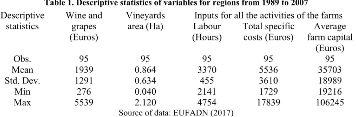
Descriptive statistics for the data used in this analysis are presented in Table 1. Table 1. Descriptive statistics of variables for regions from 1989 to 2007
Inputs for all the activities of the farms Descriptive statistics Wine and grapes (Euros) Vineyards
area (Ha) Labour (Hours) Total specific costs (Euros) Average farm capital (Euros) Obs. 95 95 95 95 95 Mean 1939 0.864 3370 5536 35703 Std. Dev. 1291 0.634 455 3610 18989 Min 276 0.040 2141 1729 19216 Max 5539 2.120 4754 17839 106245
Source of data: EUFADN (2017)
Of stressing that the sample farms is around 500 and 1000 in Entre Douro e Minho and Beira litoral, Trás-os-Montes and Beira interior, and Ribatejo e Oeste (in this region changed to 200-500 after the year 2000). In Alentejo and Algarve, and Açores and Madeira the sample is around 200 and 500.
In this work we studied the SPF function proposed by Aigner et al. (1977) and Meeusen and van Den Broeck (1977). Although, we used an extension of the original model established by Battese and Coelli (1992), that is typically used when panel data is available to explain the change in TE (Battese and Coelli, 1995). The used model can be represented as:
(1) where (1) is a Cobb and Douglas (1928) function, being the Yit the wine and grape p roduction in euros of the i-th region in the t-th year; α is the constant; β is the unknown parameters to be estimated, being X1 the vineyard area in hectares; X2 represents the labour in hours; X3 the average farm capital in euros; and X4 the total specific costs in euros; vit is the random error and uit is the non-negative random variable, associated with technical inefficiency in production of firms in the industry involved. The selected input variables of this model are the most consensual in the literature that affects the TE of the vineyard sector.
When this model is estimated, the TE is given by:
(2) The calculations of the model (1) and (2) were performed with resource to the SFA (time-varying decay) and using Stata (2017) software. Time-(time-varying decay models allow for changes in the TE over the considered period and the pertinence of these models is verified through the eta values (Battese and Coelli, 1992). Eta refers to time-varying inefficiency effects and positive values signify that the firms improve their TE over time.
In this study we also used the Malmquist (1953) index, which was introduced by Caves et al. (1982) with resource to DEA model (Fare et al., 1994) using the DEA Program (DEAP) 2.1 version. The DEAP allows the application of Malmquist DEA methods to panel data to calculate indexes of total factor productivity (TFP) change divided in efficiency change and technical change. The efficiency change represents the deviations of best practice frontier, while the technical change reflects the frontier shift over time, so the efficiency change reflects the “catching-up” effect, while technical change reflects “frontier shift” effect (Sellers-Rubio et al., 2016). The Malmquist index is estimated using distance functions and through the available panel data it allows the study of the changes in efficiency on different regions of Portugal. An input-oriented model was used to obtain an efficient unit based on a proportional decrease of its input, while the outputs proportions remain unchanged (Coelli et al., 2005).
The Malmquist index quantifies the change in total factor productivity (TFP) between two data points by calculating the distance ratio of each point relative to a common frontier. According to Grifell-Tatjé and Lovell (1996), for a given unit, the (product-oriented) index of Malmquist TFP between periods t (base period) and t+1 is given by:
1/2 t t 1 t 1 t 1 t 1 t t t t 1 t 1 t t t t 1 t 1 t 1 t t,
)
x
,
(y
d
)
x
,
(y
d
)
x
,
(y
d
)
x
,
(y
d
=
)
x
,
y
,
x
,
(y
M
×
+ + + + + + + + + (3))
x
,
y
,
x
,
(y
M
t,t+1 t+1 t+1 t t is the geometric mean of two Malmquist indexes (ratiosbetween distance functions), adopting the first as reference technology of period
t
and the second one of periodt
+
1
. A value of the Malmquist index greater, equal or less than one indicates the occurrence of growth, stagnation or decline of TFP.where (1) is a Cobb and Douglas (1928) function, being the Yit the wine and grape p roduction in euros of the i-th region in the t-th year; α is the constant; β is the unknown parameters to be estimated, being X1 the vineyard area in hectares; X2 represents the labour in hours; X3 the average farm capital in euros; and X4 the total specific costs in euros; vit is the random error and uit is the non-negative random variable, associated with technical inefficiency in production of firms in the industry involved. The selected input variables of this model are the most consensual in the literature that affects the TE of the vineyard sector.
When this model is estimated, the TE is given by:
(2) The calculations of the model (1) and (2) were performed with resource to the SFA (time-varying decay) and using Stata (2017) software. Time-(time-varying decay models allow for changes in the TE over the considered period and the pertinence of these models is verified
through the eta values (Battese and Coelli, 1992). Eta refers to time-varying inefficiency effects and positive values signify that the firms improve their TE over time.
In this study we also used the Malmquist (1953) index, which was introduced by Caves et al. (1982) with resource to DEA model (Fare et al., 1994) using the DEA Program (DEAP) 2.1 version. The DEAP allows the application of Malmquist DEA methods to panel data to calculate indexes of total factor productivity (TFP) change divided in efficiency change and technical change. The efficiency change represents the deviations of best practice frontier, while the technical change reflects the frontier shift over time, so the efficiency change reflects the “catching-up” effect, while technical change reflects “frontier shift” effect (Sellers-Rubio et al., 2016). The Malmquist index is estimated using distance functions and through the available panel data it allows the study of the changes in efficiency on different regions of Portugal. An input-oriented model was used to obtain an efficient unit based on a proportional decrease of its input, while the outputs proportions remain unchanged (Coelli et al., 2005).
The Malmquist index quantifies the change in total factor productivity (TFP) between two data points by calculating the distance ratio of each point relative to a common frontier. According to Grifell-Tatjé and Lovell (1996), for a given unit, the (product-oriented) index of Malmquist TFP between periods t (base period) and t+1 is given by:
1/2 t t 1 t 1 t 1 t 1 t t t t 1 t 1 t t t t 1 t 1 t 1 t t,
)
x
,
(y
d
)
x
,
(y
d
)
x
,
(y
d
)
x
,
(y
d
=
)
x
,
y
,
x
,
(y
M
×
+ + + + + + + + + (3))
x
,
y
,
x
,
(y
M
t,t+1 t+1 t+1 t t is the geometric mean of two Malmquist indexes (ratiosbetween distance functions), adopting the first as reference technology of period
t
and the second one of periodt
+
1
. A value of the Malmquist index greater, equal or less than one indicates the occurrence of growth, stagnation or decline of TFP.4. Results
The table 2 presents the results of the model (1). Its analysis shows that the wine and grape productions are mainly explained by the vineyard area and by the average farm capital (statistically significant). These results reveals the importance of the efforts made to modernize the farms, namely with the structural financial supports from the Community Support Frameworks applied in the Portuguese agricultural sector. The other inputs (labour and specific costs) are not statistically significant. Probably this situation occurs because these inputs reflect all the activities of the farm, instead only from the vineyard activity. All parameters have a positive signal, which means that the increase of the inputs (average farm capital, labour and vineyard area) allows an increase of the production, with the exception of the specific costs that have an inverse relationship with the production of wine and grapes. However, the values of the parameters show the pertinence of the model, namely the results for the parameter gamma. They reveal a model constant to the scale (1.082) which means that the increase in the quantity of use of the inputs determines a proportional increase of the quantity of the output.
Table 2. Results considering SFA of production function (time-varying decay), across the period 1989-2007 and for five Portuguese regions, with the logarithm of wine and grape productions as
dependent variable
Variables Parameters and statistical t
Constant 3.484 (1.070)
Logarithm of vineyard area 0.550* (9.330)
Logarithm of labour 0.033 (0.090)
Logarithm of total specific costs -0.052 (-0.400) Logarithm of average farm capital 0.447* (2.310)
/mu 0.100 (1.220) /eta 0.109* (4.170) /lnsigma2 -2.244* (-14.570) /ilgtgamma -2.935* (-2.160) sigma2 0.105 Gamma 0.050 sigma_u2 0.005 sigma_v2 0.100
Note: *, statistically significant at 5%. Source of data: EUFADN (2017).
The table 3 presents the results for TE (time-varing decay) for the Portuguese regions over the period 1989-2007.
Table 3. Results for TE (time-varying decay), across the period 1989-2007 and for five Portuguese regions Year Entre Douro e Minho and Beira Litoral Trás-os-Montes and Beira interior Ribatejo and Oeste Alentejo and Algarve Açores and Madeira Annual mean 1989 0.851 0.427 0.460 0.221 0.491 0.490 1990 0.865 0.466 0.498 0.258 0.528 0.523 1991 0.877 0.504 0.535 0.297 0.564 0.555 1992 0.889 0.541 0.571 0.336 0.598 0.587 1993 0.900 0.576 0.605 0.376 0.631 0.617 1994 0.909 0.610 0.637 0.416 0.661 0.647 1995 0.918 0.642 0.667 0.456 0.690 0.675 1996 0.926 0.672 0.696 0.494 0.717 0.701 1997 0.934 0.700 0.722 0.532 0.742 0.726 1998 0.940 0.726 0.747 0.567 0.765 0.749 1999 0.946 0.750 0.770 0.602 0.786 0.771 2000 0.952 0.773 0.791 0.634 0.806 0.791 2001 0.956 0.794 0.810 0.665 0.824 0.810 2002 0.961 0.813 0.828 0.693 0.841 0.827 2003 0.965 0.831 0.844 0.720 0.856 0.843 2004 0.968 0.847 0.859 0.745 0.870 0.858 2005 0.972 0.861 0.873 0.768 0.883 0.871 2006 0.974 0.875 0.885 0.789 0.894 0.884 2007 0.977 0.887 0.896 0.809 0.904 0.895 Annual mean 0.931 0.700 0.721 0.546 0.740 0.727 TE2007/TE1989 1,148 2,077 1,948 3,661 1,841 1,827
The results for the estimated TE (table 3) demonstrate the increase of index over the period 1989-2007, for all Portuguese regions. Entre Douro e Minho and Beira Litoral have the higher TE (annual mean of 0.931) while Alentejo and Algarve have the lower values (annual mean of 0.546). However, the most efficient group of regions - Entre Douro e Minho and Beira Litoral - only has a TE of 1.148 times for 2007 greater than 1989, while the most inefficient
group of regions - Alentejo and Algarve - has a TE 3.661 times greater in 2007, related to 1989.
The results regarding the DEA approach through the Malmquist index are in table 4. Table 4. Malmquist index results of annual and region means
Malmquist Index summary of annual means
Year Efficiency change Technical change Pure TE change Scale efficiency change Total factor productivity change 1990 0.999 0.657 0.999 1.000 0.656 1991 0.909 0.854 0.909 1.000 0.776 1992 0.863 1.462 1.068 0.808 1.261 1993 1.257 1.123 1.016 1.238 1.412 1994 1.016 0.681 1.016 1.000 0.692 1995 0.911 0.865 0.911 1.000 0.787 1996 0.960 2.021 1.097 0.875 1.940 1997 1.095 0.969 0.958 1.143 1.061 1998 1.042 0.699 1.042 1.000 0.728 1999 1.001 0.754 1.001 1.000 0.754 2000 0.862 2.467 0.967 0.891 2.126 2001 1.138 0.838 1.014 1.122 0.954 2002 0.984 0.823 0.984 1.000 0.809 2003 1.034 0.532 1.034 1.000 0.550 2004 0.894 3.280 0.935 0.956 2.934 2005 1.112 0.687 1.063 1.046 0.764 2006 1.007 0.885 1.007 1.000 0.891 2007 0.974 0.987 0.974 1.000 0.960 Mean 0.998 1.000 0.998 1.000 0.998 Accumulated 1990/2007 0.973 0.998 0.972 1.000 0.965
Malmquist Index summary of firm means
Region Efficiency change Technical change Pure TE change Scale efficiency change Total factor productivity change Entre Douro e Minho
and Beira Litoral 1.000 0.833 1.000 1.000 0.833
Trás-os-Montes and
Beira interior 0.998 0.909 0.998 1.000 0.907
Ribatejo e Oeste 1.000 1.008 1.000 1.000 1.008
Alentejo and Algarve 0.997 1.056 0.997 1.000 1.052
Açores and Madeira 0.998 1.240 0.998 1.000 1.237
Mean 0.998 1.000 0.998 1.000 0.998
On the one hand, the analysis reveals that, in an annual perspective, the TFP increased in 1992 (because of the technical change), 1993 (in consequence of increases of all indexes), 1996 (strong increase in the technical change), 1997 (increase in the efficiency change, derived from the scale efficiency change) and strongly in 2000 and 2004 (because of greater increases in the technical change). On the other hand, TFP decreased in the other years, due to the technical change, and in 2007 due to the efficiency change. Considering the mean and accumulated values over the analysed period and for the five Portuguese regions, it is observed that the TFP decreased slightly because of small decreases in the efficiency, derived from the efficiency change, more precisely of the pure technical efficiency.
In any case, the TFP shows an increasing trend during the period in terms of regional analysis. Ribatejo and Oeste, Alentejo and Algarve, and Açores and Madeira improved their TFP derived from the increases in the technical change. However, the TFP of Entre Douro e
Minho and Beira Litoral, and Trás-os-Montes and Beira Interior regions decrease due essentially to the decrease of technical change.
The joint analyse of the previous tables (3 and 4) emphasize different results. While the SFA (table 3) shows the increasing of efficiency, the Malmquist index (table 4) shows that the efficiency productivity index do not change over the period 1989-2007. The gains of efficiency, through SFA (table 3) decrease in last years, from 0.810 (2001) to 0.895 (2007), in annual mean values. Although, the Malmquist index (table 4) had more loses in the efficiency change, with indexes of 0.863 (1992), 0.862 (2000) and 0.894 (2004), precisely the years closest to the most important CAP reforms.
In terms of regional analysis, while the SFA shows that the Entre Douro e Minho and Beira Litoral are the most technical efficient region (table 3) and with some growth, the Malmquist index shows that TFP change decreases over the period 1989 to 2007, due to the technical change (table 4). However, the Alentejo and Algarve is the most inefficient regions through SFA (table 3), but with the greatest progress. The Malmquist index emphasizes this situation, once it reveals a positive change in TFP for the same regions.
5. Conclusions
The estimation of productivity efficiency of Portuguese regions over the period 1989-2007 conduct to the different results when is used SFA and DEA through Malmquist index. Based on the first approach all regions improve TE over the period 1989-2007, while it is noted a decrease when calculated the Malmquist index or TFP change due to the efficiency change. It means that some farms have difficulties in approaching the best frontier of production.
In regional terms, SFA shows the improved technical progress for all Portuguese regions, especially in the most inefficient regions, such as Alentejo and Algarve, while Malmquist index reveals that only two groups (Açores and Madeira; and Alentejo and Algarve) enhanced the TFP change and other two regions decreased the index (Entre Douro e Minho and Beira litoral; and Trás-os-Montes and Beira Interior). All these changes in Malmquist index are derived from technical change that reveals that some regions had technological progress and others had loses in efficiency due to the non-modernization of its production technologies. 6. References
Aigner, D., Lovell, C. K., and Schmidt, P. 1977. “Formulation and estimation of stochastic frontier production function models”, Journal of Econometrics, 6 (1): 21-37.
Aparicio, J., Borras, F., Pastor, J. T., and Vidal, F. 2013. “Accounting for slacks to measure and decompose revenue efficiency in the Spanish Designation of Origin wines with DEA”. European Journal of Operational Research, 231 (2): 443-451.
Battese, G. E., and Coelli, T. J. 1992. “Frontier production functions, technical efficiency and panel data: with application to paddy farmers in India”. Journal of Productivity Analysis, 3: 153-169. Battese, G. E., and Coelli, T. J. 1995. “A model for technical inefficiency effects in a stochastic frontier
production function for panel data”. Empirical Economics, 20: 325-332.
Brandano, M. G., Detotto, C., and Vannini, M. 2012. “Comparative Efficiency of Producer Cooperatives and Conventional Firms in a Sample of Quasi-Twin Companies” (No. 201228). Sardinia: Centre for North South Economic Research, University of Cagliari and Sassari. Caves, D. W., Christensen, L. R., and Diewert, W. E. 1982. “The economic theory of index numbers
and the measurement of input, output, and productivity”. Econometrica: Journal of the Econometric Society, 50 (6): 1393-1414.
Cobb, C. W., and Douglas, P. H. 1928. “A Theory of Production”. American Economic Review, 18 (Supplement): 139-165.
Coelli, T. J., Rao, D. S. P., O'Donnell, C. J., and Battese, G. E. 2005. “An Introduction to Efficiency and Productivity Analysis”. Springer Science & Business Media.
Coelli, T., and Sanders, O. 2013. “The technical efficiency of wine grape growers in the Murray-Darling Basin in Australia”. In Giraud-Héraud, E. and Pichery, M. C. (eds), Wine Economics. Quantitative Studies and Empirical Applications. Hampshire (UK): Palgrave Macmillan, 231-249. Conradie, B., Cookson, G., and Thirtle, C. 2006. “Efficiency and farm size in Western Cape grape
production: pooling small datasets”. South African Journal of Economics, 74: 334-343.
Cullinane, K., Wang, T. F., Song, D. W., and Ji, P. 2006. “The technical efficiency of container ports: comparing data envelopment analysis and stochastic frontier analysis”. Transportation Research Part A: Policy and Practice, 40 (4): 354-374.
EUFADN: European Union Farm Accountancy Data Network, 2017. “European Union Farm Accountancy Data Network”. http://ec.europa.eu/agriculture/rica/ (accessed January 24, 2017). Fare, R., Grosskopf, S., and Lovell, C. K. 1994. Production Frontiers. Cambridge University Press. Farrell, M. J. 1957. “The measurement of productive efficiency”. Journal of the Royal Statistical
Society, Series A (General), 120 (3): 253-290.
Fleming, E., Mounter, S., Grant, B., Griffith, G., and Villano, R. 2014. “The New World challenge: Performance trends in wine production in major wine-exporting countries in the 2000s and their implications for the Australian wine industry”. Wine Economics and Policy, 3 (2): 115-126. Freitas, R. 2014. “Sobre a eficiência dos países produtores de uvas para vinho na União Europeia: uma
aproximação DEA em duas etapas”. Masters Dissertation, Catholic University of Portugal. Fuensanta, M. J. R., Sancho, F. H., and Marco, V. S. 2015. “In vino veritas: competitive factors in
wine-producing industrial districts”. Investigaciones Regionales, (32), 149.
GAIN: Global Agricultural Information Network. 2015. Global Agricultural Information Network, Wine Annual Report and Statistics 2015. USDA Foreign Agricultural Services, GAIN Report Number: IT1512.
Grifell-Tatje, E., and Lovell, C. K. 1996. “Deregulation and productivity decline: The case of Spanish savings banks”. European Economic Review, 40 (6): 1281-1303.
Henriques, P.D.S., Carvalho, M.L.S., and Fragoso, R.M.S. 2009. “Technical efficiency of Portuguese wine farms”. New Medit, 8 (1): 4-9.
Herrera, B., Gerster-Bentaya, M., and Knierim, A. 2016. “Stakeholders’ perceptions of sustainability measurement at farm level”. Studies in Agricultural Economics, 118: 131-137.
József, T., and Péter, G. 2014. “Is the New World more efficient? Factors influencing technical efficiency of wine production”. Studies in Agricultural Economics, 116: 95-99.
Malmquist, S. 1953. “Index numbers and indifference surfaces”. Trabajos de estadística, 4 (2): 209-242.
Manevska-Tasevska, G. 2013. “Product assortment and the efficiency of farms”. In Giraud-Héraud, E. and Pichery, M. C. (eds), Wine Economics. Quantitative Studies and Empirical Applications. Hampshire, UK: Palgrave Macmillan, 250-265.
Marta-Costa, A., and Silva, E. (eds.) 2013. Methods and Procedures for Building Sustainable Farming Systems: Application in the European Context. Netherlands: Springer Editions.
Marta-Costa, A. A. 2010a. “Agricultura Sustentável III: Indicadores”. Revista de Ciências Agrárias, 33 (2): 90-105.
Marta-Costa, A. A. 2010b. “Sustainability Study for the Rearing of Bovine Livestock in Mountainous Zones”. New Medit, 9 (1): 4-12.
Meeusen, W., and van Den Broeck, J. 1977. “Efficiency estimation from Cobb-Douglas production functions with composed error”. International economic review, 18 (2): 435-444.
Moreira, V. H., Troncoso, J. L., and Bravo-Ureta, B. E. 2011. “Technical efficiency for a sample of Chilean wine grape producers: A stochastic production frontier analysis”. Ciencia e Investigación Agraria, 38 (3): 321-329.
Mourão, P. R., and Martinho, V. D. 2016. “Scoring the efficiency of Portuguese wine exports – an analysis recurring to Stochastic Frontier Models”. Ciência Téc. Vitiv., 31 (1): 1-13.
OIV: International Organisation of Vine and Wine. 2016. “OIV Statistical Report on World Vitiviniculture: World Vitiviniculture Situation”. http://www.oiv.int/public/medias/5029/world-vitiviniculture-situation-2016.pdf (accessed January 1, 2016).
PTFADN: Portuguese Farm Accountancy Data Network. 2017. “Portuguese Farm Accountancy Data Network”. http://www.gpp.pt/index.php/rica/rede-de-informacao-de-contabilidades-agricolas-rica (accessed January 24, 2017).
Sampaio, A. 2013. “Review of frontier models and efficiency analysis: a parametric approach”. In Mendes, A., Silva, E. and Santos, J. (eds), Efficiency Measures in the Agricultural Sector, Springer Edition, 13-35.
Sellers-Rubio, R., and Más-Ruiz, F. J. 2015. “Economic efficiency of members of protected
designations of origin: sharing reputation indicators in the experience goods of wine and cheese”. Review of Managerial Science, 9 (1): 175-196.
Sellers-Rubio, R., Alampi Sottini, V., and Menghini, S. 2016. “Productivity growth in the winery sector: evidence from Italy and Spain”. International Journal of Wine Business Research, 28 (1): 59-75.
Silva, E., Mendes, A., and Santos, J. 2013. “Efficiency measures in the agricultural sector: the beginning”. In Mendes, A., Silva, E. and Santos, J. (eds), Efficiency Measures in the Agricultural Sector, Springer Edition, 3-12.
Stata. 2017. “Data Analysis and Statistical Software”. http://www.stata.com/ (accessed January 24, 2017).
Tóth, J., and Gál, P. 2014. “Is the New Wine World more efficient?”. Studies in Agricultural Economics, 116 (2): 95-99.
Vidal, F., Pastor, J. T., Borras, F., and Pastor, D. 2013. “Efficiency analysis of the designations of origin in the Spanish wine sector”. Spanish Journal of Agricultural Research, 11 (2): 294-304. Acknowledgements:
This work was supported by the project NORTE-01-0145-FEDER-000038 (INNOVINE & WINE – Vineyard and Wine Innovation Platform) and by European and Structural and Investment Funds in the FEDER component, through the Operational Competitiveness and Internationalization Programme (COMPETE 2020) [Project No 006971 (UIC/SOC/04011)]; and national funds, through the FCT – Portuguese Foundation for Science and Technology under the UID/SOC/04011/2013.
View publication stats View publication stats