* Corresponding author. Tel. (+9821)66413034; Fax: (+9821)66413025 E-mail addresses: [email protected] (S. M. T. Fatemi Ghomi) © 2010 Growing Science Ltd. All rights reserved. doi: 10.5267/j.ijiec.2010.02.002
Contents lists available at GrowingScience
International Journal of Industrial Engineering Computations
homepage: www.GrowingScience.com/ijiec
Economic lot scheduling problem with consideration of money time value
Maryam Mokhlesiana*, Seyyed Mohammad Taghi Fatemi Ghomia and Fariborz Jolaib
a
Department of Industrial Engineering, Amirkabir University of Technology, 424 Hafez Avenue,, Tehran, Iran
b
Department of Industrial Engineering, College of Engineering, University of Tehran, Tehran, Iran
A R T I C L E I N F O A B S T R A C T
Article history: Received 1 April 2010 Received in revised form 10 May 2010
Accepted 10 May 2010 Available online 24 May 2010
The economic lot scheduling problem (ELSP) is a challenge between sequencing and lot sizing. In this problem, several products must be produced on a single machine in a cyclical production pattern and the primary goal is to minimize the total setup and holding expenditures. Since time affects the value of money, it is necessary to take into account the time value of money when gradual payment is the case. In this paper, a new ELSP model with the consideration of the time value of money is considered. The proposed model of this paper is formulated as a nonlinear mixed integer model and a hybrid GA is presented to solve the resulted model for large-scale problems. The proposed method is solved for some benchmark problems for large-scale problems.
©2010 Growing Science Ltd. All rights reserved. Keywords:
Economic lot scheduling problem Discount cash flow
Genetic algorithm Sequence dependent Hybrid method Metaheuristic
1. Introduction
The economic lot scheduling problem (ELSP) deals with scheduling of multi products on a single machine. In essence, the purpose of ELSP is to minimize the costs of holding and setup while the demand of each product in each cycle is satisfied. The solution involves determining a consistent and repetitive production schedule for all products to meet the necessary demand (Chatfield (2007)).
1.1. Literature review
Previous research studies on ELSP can be classified in two main areas:
1. Improvement on the classic ELSP model 2. Developing methods to solve ELSP
1. Improvement on the classic ELSP model: Dobson (1992) and Wagner and Davis (2002) reviewed
variety of modifications by considering common parameters as decision variables in manufacturing systems modeling. The effect of various production rates on the ELSP was investigated by Silver (1990), Moon et al. (1991), Gallego (1993), Khouja (1997), and Moon and Christy (1998). These studies showed the profitability of decreasing the production rate of an under-utilized facility. Silver (1995) and Viswanathan and Goyal (1997) studied the shelf life constraint on a single production facility for production of multiple items in repetitive cycles. Allen (1990) proposed a graphical approach to find the optimal production rate and cycle time for a production facility producing only two products. Faaland et al. (2004) introduced a new modeling framework for the ELSP that allows for lost sales leading to higher profits. They also considered the set-up times in the model with no investment option and showed that lost sales could be profitable, even where deterministic production and demand rates are considered. Gallego and Moon (1992) studied the trade-off between reducing the set-up time and increasing the set-up cost by externalizing the set-up operations with an increase in set-up cost. Moon (1994) considered a reduction in set-up time by a onetime investment in an ELSP model. Hwang et al. (1993) and Moon (1994) developed an ELSP model where both the set-up time reduction and quality improvement in the investment set-up cost are considered. Moon et al. (1998) also proposed a stabilized ELSP method for the production rate. In a later study, Moon et al. (2002) considered an unreliable production equipment in the ELSP, where production starts with an ‘‘In-Control’’ state and could face with an ‘‘Out-of Control’’ state. Giri et al. (2003) also investigated preventive and corrective maintenance, as well as the related costs. Teunter et al. (2008) studied the economic lot scheduling problem with two production sources, manufacturing and remanufacturing, for which operations performed on separate, dedicated lines. Piñeyro and viera (2010) investigated a lot-sizing problem with different demand streams for new and remanufactured items, in which the demand for remanufactured items can be also satisfied by new products, but not vice versa.
2. Developing methods to solve ELSP: During the last four decades, there have been tremendous
two heuristic methods, DH and GA. Raza and Akgunduz (2008) presented a new meta-heuristic based on the simulated annealing (SA) algorithm to solve the ELSP. Jenabi et al. (2007) addressed the economic lot sizing and scheduling problem in flexible flow lines with unrelated parallel machines over a finite planning horizon. Aiming to obtain the optimal solution particularly for medium and large-sized problems, the paper proposed two algorithms: a hybrid genetic algorithm (HGA) and a simulated annealing (SA). Sun et al. (2009) proposed a genetic algorithm for solving the ELSP problem. The genetic algorithm used an integer encoding scheme which encoded the basic period only, implicitly. This lean representation cut down the search space by one dimension to speed up the search. Teunter et al. (2009) presented a complex algorithm for the multi-item ELSP with two sources of production: manufacturing of new items and remanufacturing of returned items which determined the optimal solution within the class of policies with a common cycle time and a single (re)manufacturing lot for each item in each cycle. This paper contributes to the research literature discussed by considering the time value of money in solving the ELSP where monitory unit in different times has different values. Considering the time value of money has the two following advantages:
1. The possibility of comparing the monitory unit in different times 2. The possibility of gradual payment of costs
In fact, there has not been any research study conducted in the area of ELSP which takes into account the time value of money. Therefore, we investigated the effect of this factor on classic model of ELSP and then re-modeled the ELSP considering the time value of money using the discounted cash flow approach. In this paper, we aim to demonstrate the impact of the time value of money. Moreover, we propose a new way to combine the genetic algorithm and role of design experiments to enhance the efficiency of algorithm. This paper has the following structure. In section 2, we define the classic ELSP model based on the existing literature. In section 3, we take into account the time value of money for set-up and holding costs using the discounted cash flow approach. Section 4 is focused in developing a hybrid genetic algorithm to solve the new model. In section 5, we present a numerical example to provide a better understanding of the problem and then explain the advantages of the proposed model. Finally, section 6 is devoted to conclusion and recommendation for future studies.
2. The economic lot scheduling problem (ELSP)
The purpose of the ELSP is to determine a production cycle of ith , , … , product in a repetitive schedule. A repetitive schedule is achieved if there is a time period
for each product that represents the time between successive production runs (batches or “lots”) of item i. In this paper we consider the same cycle time for all products (common cycle approach).
2.1. Notations
The parameters for the classic ELSP are as follows:
N Number of products j Sequence index
i Product index
i
d Demand rate for product i in units per day
i
p Production rate for product i in units per day
i
h Holding cost for product i
jk
cs Setup cost to switch from production of product j to the next product ( )
jk
c
t Cycle time
s j
t Start time for the product produced in the jth position of the sequence
e j
t End time for the product produced in the jth position of the sequence
j
q Lot size of product in the jth position of the sequence
p j
t Processing time of product in the jth position of the sequence
M A big number
r Compound interest rate
2.2. Conditions and assumptions
Conditions and assumptions in the classic ELSP are as follows:
1. Only one item i can be produced at a time; 2. Shortage is not allowed;
3. Setting up for a certain item incurs both a specific setup cost csijand setup time ( s i
t );
4. Setup cost and setup time are determined and sequence dependent;
5. Demand rate (di) and production rate (pi)are known and constant for all items (di≤pi);
6. All demand must be met;
7. Holding costs (hi) are determined and constant;
8. Production facility is assumed failure free and always produces the highest products.
2.3. Objective function
The cost per unit time for item i is defined by (Chatfield (2007)) as follows,
= setup cost + holding cost,
where the first term is the setup cost of the ith product in a given sequence per unit time and the second term is the holding cost of the ith product (based on the economic production quantity (EPQ) model). We consider the cost in any cycle by multiplying (1) by where is the cycle time of any
product based on the EPQ model. The total cost per cycle is the sum of (1) for all productions.
The total cost function used for the economic order quantity, is as follows:
. (2)
The objective is to minimize the setup and holding costs by determining the optimal sequence, , and . Such a problem is complex due to the nonlinear relationship in the cost function and the imposition of the constraints regarding capacity limitations and demand satisfaction requirements.
2.4. Solutions feasibility
Although the ELSP has been simplified through some restrictions such as deterministic demand and sequence independent setup times, it still remains a difficult problem due to the fact that it does have any closed form expression yet. Also, testing its solutions for feasibility is NP-complete (Chatfield (2007)). Two or more products may compete for one facility at the same time under the following conditions:
1. The load on the facility must not exceed the capacity (capacity constraint). On the other hand, the load must not be higher than the facility’s capacity.
2. The product lot size must be large enough to satisfy the demand occurring between two successive production runs to avoid shortage.
2.5. Proposed Model
There are a variety of formulations for the ELSP. We will use the formulation which is compatible to the conditions and assumptions of common cycle approach:
subject to
(3)
, , … , (4)
, , … , (5)
, , … , (6)
, , … , (7)
, , … , (8)
, (9)
, (10)
, (11)
, (12)
, . (13)
The objective function (3) minimizes the average setup and holding costs for the schedule. The constraint sets (4) and (5) impose that each of the products must be assigned to only one location and vice versa. The constraint set (6) indicates that the lot size for each product must be produced during the processing time (the time between start and end of the production). It also shows that the production of each product is non-disruptive. The constraint set (7) ensures that the lot size satisfies the demand of each cycle. Constraint (8) enforces that the start time of producing a product must be greater than the end time of producing the previous product ( ) plus the setup time , . Constraint (9) requires that the production of the first product in the sequence starts after the machine setup has been completed. Constraint (10) indicates that all products must be produced in every cycle. It also ensures that the end time of producing the last product is less than the cycle time. Constraints (11) to (13) show the relation between and . Based on constrains (11) and (12), if and then is either 0 or 1. Since the constraint (13) ensures that is equal or larger than 1. Therefore, if product i is produced in location l ( ) and product u is produced in location l+1
( ), i and u are consecutive.
3. Inventory models with the time value of money
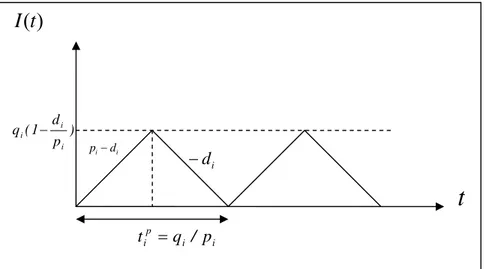
In developing a mathematical model for inventory control, it is usually assumed that the payment are made to the suppliers immediately after receiving the orders. However, suppliers often allow a certain period of time for settling the account on a day-to-day basis (Aggarwal and Jaggi (1995)). During this period, suppliers consider the time value of money for the costs and impose it to their accounts. We do not consider this type of delay on the payment for our model because we re-modeled the classic ELSP based on its primary assumptions and considerations, and then we add the time value of money. Hence, this paper considers on time payments and for the sake of simplicity, we use the net present value of the costs. In order to take into account the time value of money in the inventory costs, the discounted cash-flow approach is applied. In this approach, the unit of monetary at time has the present worth (Wee and Law (1999)). To conduct the computations, we calculate the present worth of costs considered in the classic ELSP and then rewrite the model. The graphical representation of the production system is shown in Fig 1.
Fig 1. Graphical representation of production system
I
(
t
)
t
) p d 1 ( q
i i
i −
i i p
i q / p
t =
i
i d
p−
i
d −
3.1. The present value of the setup cost
The setup cost of the first product in the sequence, , occurs at the start of the cycle (t=0), the second one occurs at and so on. Therefore, the present value of the setup cost is calculated as follows,
, (13)
, (14)
3.2. Present value of the holding cost
When the production process for each product is completed, it must be held. Since the holding cost is paid at the start of the holding inventory, the present value of the holding cost is computed as follows:
. (15)
3.3. The ELSP model considering the time value of money
In this section, we want to minimize the present value of the holding cost plus the present value of the setup cost for the infinite planning horizon. Therefore, we rewrite the formulation of ELSP's costs in planning horizon as follows:
/ / . (16)
Equation (16) calculates the present value of the costs whereas equation (2) is for the costs of the classic ELSP. This paper only focuses on the costs of the classic ELSP. Other cost items such as procurement costs are not taken into account so that we could compare our model with the classic ELSP more precisely. Also, only the costs incurred during the period of production run are considered here. So the costs incurred before the production run is eliminated from the model. Since costs appear only in the objective function, the constraints subjected to our model are similar to the constraints subjected to of the classic model. Solving this model determines the sequence of production, quantity of any product (lot size) and time cycle of products.
4. Development of a hybrid genetic algorithm
4.1. Genetic algorithm procedure
algorithms, a population of individuals (potential solutions) undergoes a sequence of unary (mutation type) and higher order (crossover type) transformations. These individuals strive for survival. A selection scheme directs the GA towards promising fitter individuals to select the next generation. This new generation contains a higher proportion of the characteristics possessed by the "good" members of the previous generation; in this way, good characteristics are spread over the population and mixed with other good characteristics. After some number of generations, the program converges and the best individual represents a near optimum solution. Fig. 2 shows the GA procedure (Khouja et al. (1998)).
Procedure: Genetic Algorithm Begin
t←0
initialize P(t)
evaluate P(t)
while (recombination condition) do recombination P(t)to yield C(t)
evaluate C(t)
select P(t+1)from P(t)and C(t)
end end
Fig. 2.The procedure of a GA
4.2. Genetic algorithms’ components
Each GA has the following components:
1. Chromosome representation: the GA shows the solution in a string called “chromosome”.
There are different procedures to show the chromosome. We will use one of these procedures called “ordinal representation”. In this procedure, each bit of chromosome is a number showing the sequence.
2. Initial population: the first stage in the GA is the generation of initial population. A set of chromosome is defined as a “population”. The initial population can be generated randomly. The number of chromosome in the population is named “the population size”.
3. Selection and fitness function: each chromosome in the population must be evaluated by
fitness function. The chromosome with larger fitness has more chance to be selected for the next population
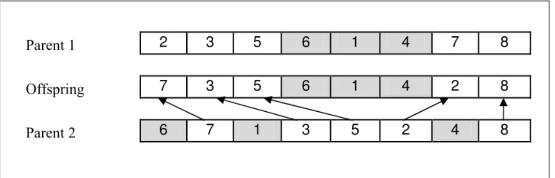
GA operators: The crossover operator first chooses pairs of individuals among all the individuals in the population with a predefined probability (the crossover rate denoted by ). In the literature, linear order crossover (LOX) is the most frequently-used operator for crossover operation when the chromosome representation is ordinal. After selecting parents for crossover, the following steps must be performed for LOX crossover (Gen and Cheng (2000)). Also, Fig. 3 shows an example of the LOX operator.
Step1: Select a job sub-sequence randomly from one of the parents.
Step2: Copy this job sub-sequence in offspring chromosome.
8 7 4 1 6 5 3 2 Parent 1 8 2 4 1 6 5 3 7 Offspring 8 4 2 5 3 1 7 6 Parent 2
Fig. 3 LOX operator
Next, we apply the mutation operator to the population that just experienced the crossover operator. The mutation operator randomly chooses one parent among the individuals in the population with a fixed mutation rate (denoted by ). Then, the inversion mutation operator is used as follows:
Step1: Select two positions in parent chromosome randomly.
Step2: Invert all elements between two selected positions.
Fig. 4 shows an example of the inversion mutation operator.
8 6 3 4 7 5 1 2 Parent 8 6 5 7 4 3 1 1 Offspring
Fig. 4. Inversion mutation operator
4. The parameters setting: A statistical DOE is used to analyze the performance of the GA. This algorithm will be explained in section 5.
4.3. Hybrid genetic algorithm
One of the most common approaches in hybrid genetic algorithms (HGAs) is incorporating local search techniques to a main genetic algorithm’s loop of recombination and selection. Genetic algorithms are fast at global search but slow to converge. On the other hand, local search is good at fine tuning but often falls into local optimum. The hybrid approach complements the properties of genetic algorithm and local search heuristic methods. Genetic algorithms are used to perform a global search in order to escape from local optimum whereas local search is used to conduct fine tuning.
Hybridization can be done in a variety of ways, such as the following (Gen and Cheng (2000)):
3. Incorporate a local search heuristic into the basic loop of genetic algorithm, working together with mutation and crossover operators, localized optimization to improve offspring before returning it to be evaluated.
In local search approach, a comprehensive exploration of the solution space is executed by moving at each step from the present solution to another promising one in its neighborhood (Hertz and Widmer (2003)).
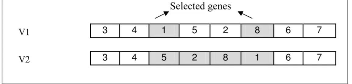
The neighborhood search (NS) used in our HGA is based on an iterative search in the vicinity of solution. Different definitions of neighbor have been presented. In our proposed HGA, insertion neighborhood is used. In this type of neighborhood, an order vector is a neighbor of a similar vector if by removing one bit of (such as ), inserting in another bit (such as ) and shifting the bits between and to left is achieved where and are randomly selected (Wang and Wu (2003)). In other word, if the number of genes is begun from left to right, the value of a selected gene with a smaller number is put in a selected gene with a larger number and the value of genes between two selected positions and larger number of gene are shifted one gene to the left. This approach is outlined as follows:
1. Call the bits of chromosome from start to end with 1 to N.
2. Select two positions of bits randomly and call them p1 and p2 (p1 > p2). 3. Remove the value of bit p1.
4. Shift the value of each of bits between p1 and p2 one bit into the left. 5. Copy the value of bit p1 in bit p2.
Figure 5 illustrates this approach.
Selected genes
7 6 8
2 5
1 4 3
V1
7 6 1
8 2
5 4 3
V2
Fig.5. NS and insertion method
4.4. Solution representation
The chromosome in our algorithm has N bits (N is the number of products). The ith bit shows the product number produced in the ith position of the sequence. For example, in a 3-product problem, the chromosome {312} can be used to represent the solution in which product 3 is the first product to be produced followed by product 1 and then product 2.
4.5. The proposed HGA
Sequence Lot size Start time End time Cycle time
…
…
…
…
Fig. 6. Representation of solution
The stages of our algorithm are as follows:
1. Determine the proper values of GA parameters
2. Represent the sequence with chromosomes in an ordinal representation 3. Make an initial population randomly
4. Solve the model to calculate other variables and compute fitness value 5. Select and duplicate chromosomes to perform the crossover operator 6. Perform the crossover operator
7. Apply Neighborhood Search (NS) method to replace any child created by crossover with its better neighbor
8. Select chromosomes randomly to perform the mutation operator 9. Perform the mutation operator
10.Apply Neighborhood Search (NS) method to replace any child created by mutation with its better neighbor
11.Compare fitness value of all improved chromosomes with the current population, choose population size of the best available solutions as the size of the next population and save the best available solution
12.Repeat stages 5 to 11 until termination criteria are achieved. Terminate the algorithm if the maximum number of generation (max_gen) or the maximum number of generation without improvement (max_no_improve) is equal to the predefined number
5. Using DOE for parameter tuning
The efficiency of an algorithm depends on choosing the best parameters in order to prevent premature convergence, ensure diversity in the search space and intensify the search around interesting regions. This section explains the implementation of our proposed approach to find the best tuning parameters of the proposed method. In order to reduce the number of combinations, some parameters are fixed as priori based on the preliminary tests. This is because considering all parameters increases the calculation volume in ANOVA and makes the process more complex. We applied parameters tuning only for the population size (pop_size), and max_no_improve. Each time we ran these tests, we changed the value of one parameter, fixed the others and saved the value of the objective function and CPU time. After performing these tests for 90 test problems, we found that some parameters such as mutation rate and the maximum number of generation did not change the two above-mentioned values significantly. Hence, we considered these values to be fixed and performed ANOVA on other parameters. Other parameters are set as follows:
max-generation=500
.
To set the above parameters, we considered some of the most widely-used parameters in the literature. Next, the preliminary tests were performed to determine the parameters with better effects on the objective function value and the running time.
Table 1 Levels of DOE
Levels Lable
Factors
100 10n
50
A
pop_size
0.9 0.8
0.7
B
100 50
20
C
max_no_imrpove
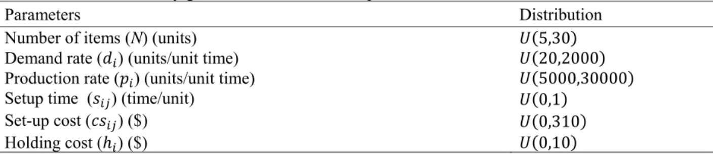
For each combination of the three factors under study, 30 randomly selected problems were solved and responses were measured. These problems were selected from a given data set shown in Table 2.
Table 2
Distribution for randomly generated data for the test problems
Parameters Distribution
Number of items (N) (units) ,
Demand rate ( ) (units/unit time) ,
Production rate ( ) (units/unit time) ,
Setup time ( ) (time/unit) ,
Set-up cost ( ) ($) ,
Holding cost ( ) ($) ,
Table 3 shows the ANOVA results where the response is the value of fitness function and α=0.90.
Table 3
33 factorial design
Sources df SS MS F
A 2 2.92×10⁵ 1.46×10⁵ 0.0044
B 2 2.86×10⁹ 1.43×10⁹ 43.43∗
A×B 4 2.92×10⁵ 7.31×10⁴ 0.0022
C 2 1.40×10⁶ 7.04×10⁵ 0.021
A×C 4 1.08×10⁶ 2.72×10⁵ 0.0083
B×C 4 6.83×10⁵ 1.70×10⁵ 0.0052
A×B×C 8 2.85×10¹⁰ 3.57×10⁹ 108.46∗
Error 783 2.57×10¹⁰ 3.29×10⁷
It is found that changing and combination of three parameters can affect the performance of the proposed HGA. This is because the corresponding value of , , for them is less than the column F
in Table 3 and the change in the value of the others has no significant effect on the performance of the algorithm. This is because the corresponding value from statistical table , , is greater than the column F in Table 3. Therefore, for insignificant parameters, we choose values with better objective function values and running times. Then, we use Newman-Keules test (Hicks (1993)) for tuning the significant parameters from all these levels (Table 1). The results of parameter tuning are as follows:
. , , _ _
Table 4
Results of comparing HGA with LINGO
Run time of HGA (second) The times that results of HGA was
better than LINGO Size of problems
Max Mean
138.92 80.75
14 5
320.56 115.23
8 10
623.85 298.73
... 30
From Table 4, it can be seen that for small size problems (5 products) in % of times the HGA gives a better result than LINGO and for the other 53%, the results of two approaches are the same. Since for most small and medium size problems, the HGA offers significantly better results than LINGO, it can be concluded that out proposed HGA has a satisfactory performance. Note that the generalization of this remark for large size problems must be made more carefully. Due to the nonlinear nature of this problem, LINGO may converge to a local optimum. Therefore, for some test problems, the results of the HGA will be better than the LINGO's. Solving all test problems have been implemented on a personal computer with dual core processor 4400 + 2.3 GHz, 1.87 GB of RAM, and the proposed algorithms have been coded with MATLAB 7.4.0.
6. A numerical example
In this section, we present a numerical example to provide a better understanding of the problem and to show the advantages of our proposed model. We use the initial data from Bomberger’s example (Table 5). Other data were generated randomly with distribution mentioned in Table 2.
Table 5
Initial data (Chatfield (2007))
i 1 2 3 4 5 6 7 8 9 10
d (per day) 400 400 800 1600 80 80 24 340 340 400
p (per day) 30000 8000 9500 7500 2000 6000 2400 1300 2000 15000
h (per day) 0.0065 0.1775 0.1275 0.1 2.785 0.2675 1.5 5.9 0.9 0.04
CS=
. . .
. . .
. . .
. . .
. . .
. . .
. . . .
. . . .
. . . .
. . .
. . .
. . .
. . .
. . .
. . .
. . . .
. . . .
. . . .
. . .
. . .
.
. .. ..
. . .
. . .
.
. .. ..
. . . .
. . . .
.
. .. .. ..
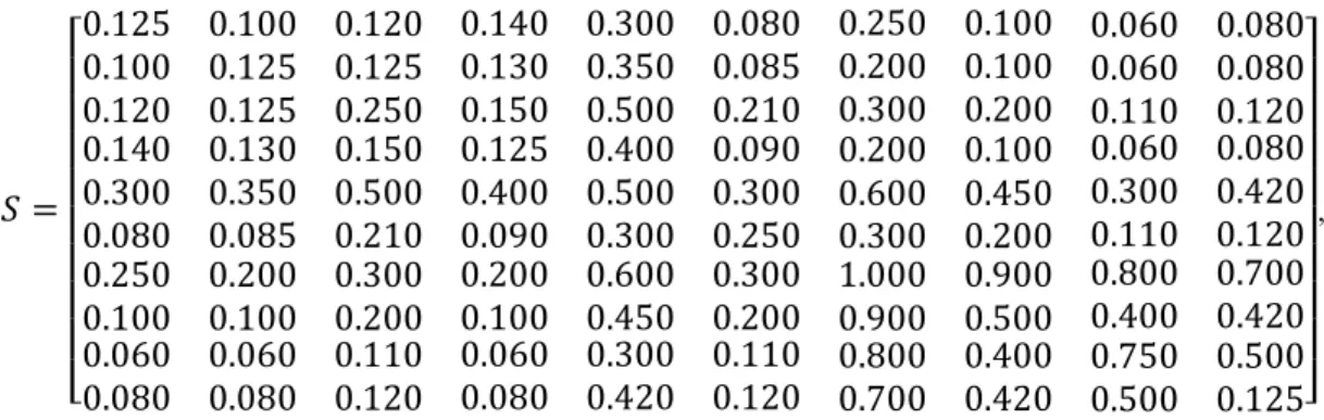
,
where S and CS are the matrices of setup costs and times for each possible sequences, respectively. For example, the setup cost and time for producing product 3 coming after 2 are 19 and 0.125. On the other hand, as described in section 2.1.1, the setup cost and the time needed to switch from producing product to the next product ( ) are represented in the kth position of row jth in these two matrices.
6.1 Analysis of results
Table 6 shows the results of model with the time value of money after 139.1 seconds running.
Table 6
Results of ELSP considering money time value (r=0.25)
Sequence 10 1 5 6 9 3 2 8 4 7
Lot size 5272 5272 1054 1054 4481 10545 5272 4481 21091 316
Start time 0.125 0.56 1 1.9 2.1 4.5 5.7 6.5 10 13.1
End time 0.5 0.7 1.5 2 4.4 5.6 6.4 9.9 12.9 13.2
Cycle time: 13.2 Total cost: 15241.2
Table 7 shows the results of model without the time value of money (classic ELSP) after 103.8 seconds running:
Table 7
Results of classic ELSP (r=0)
Sequence 10 3 2 8 1 6 5 9 4 7
Lot size 5137 10273 5137 4366 5137 1027 1027 4366 20547 308
Start time 0.125 0.587 1.7 2.5 6 6.2 6.7 7.5 9.8 12.7
End time 0.5 1.6 2.4 5.9 6.1 6.4 7.2 9.7 12.5 12.8
Cycle time: 12.8 Total cost: 14849.7
Table 8
Results of ELSP considering money time value (r=0.1)
Sequence 4 8 6 10 3 9 2 7 1 5
Lot size 21567 4583 1078 5391 10783 4583 5391 323 5391 1054
Start time 0.125 3.1 6.8 7.1 7.6 8.9 11.2 12.1 12.5 12.9
End time 3 6.6 7 7.5 8.7 11.1 11.9 12.2 12.6 13.2
Cycle time: 13.2 Total cost: 15584.06
Table 9
Results of ELSP considering money time value (r=0.3)
Sequence 10 3 8 1 5 6 2 9 4 7
Lot size 5272 10545 4481 5272 1054 1054 5272 4481 21091 316
Start time 0.125 0.6 1.9 5.5 5.9 6.6 7 7.7 10 13.1
End time 0.5 1.7 5.4 5.6 6.5 6.9 7.6 9.98 12.9 13.2
Cycle time: 13.2 Total cost: 15240.58
Table 10
The effect of parameter r
r=0.1 r=0.25 r=0.3
Total cost Cycle time Total cost Cycle time Total cost Cycle time
15584.06 13.2 15241.2 13.2 15240.58 13.2
Comparing the results indicate that taking into account the time value of money reduces the costs. Also, our model makes the gradual payment possible which, in turn, could reduce the costs from selling the products. Considering the time value of money gives more flexibility to the model resulting in lower costs.
The ELSP with the time value of money intends to increase the times because of appearing negative values of times in the power of exponential function. Hence, to minimize the objective function, these values must be increased. However, this increase is limited by constraints (5) and (6). Therefore, the proposed model has a larger cycle time.
7. Conclusion and recommendation for future studies
References
Aggarwal, S.P. & Jaggi, K.C. (1995). Ordering policies of deteriorating items under permissible delay in payments. Journal of the Operational Research Society, 46, 658-662.
Allen, S.J. (1990). Production rate planning for two products sharing a single process facility: A real world case study. Production and Inventory Management, 31, 24–29.
Aytug, H., Khouja, M., & Vergara, F.E. (2003). Use of genetic algorithm to solve production and operations management problems: A review. International Journal of Production Research, 41, 3955–4009.
Bomberger, E.E. (1966). A dynamic programming approach to a lot size scheduling problem.
Management Science, 12, 778–784.
Bourland, K.E. & Yano, C.A. (1997). A comparison of solution approaches for the fixed-sequence economic lot scheduling problem. IIE-Transactions, 29, 103–108.
Chatfield, D. (2007). The economic lot scheduling problem: A pure genetic search approach.
Computers and Operations Research, 34, 2865 – 2881.
Davis, S. (1990). Scheduling economic lot size production runs. Management Science, 36, 985-998. Dobson, G. (1987). The economic lot-scheduling problem: Achieving feasibility using time-varying
lot sizes. Operations Research, 35, 764–771.
Dobson, G. (1992). The cyclic lot scheduling problem with sequence-dependent setups. Operations Research, 40, 736–749.
Doll, C.L. & Whybark, D.C. (1973). An iterative procedure for the single-machine multi-product lot scheduling problem. Management Science, 20, 50–55.
Eilon, S. (1959). Economic batch-size determination for multi-product scheduling. Operations Research, 10, 217–227.
Elmaghraby, S. (1978). The economic lot scheduling problem (ELSP): Review and extension.
Management Science, 24, 587–598.
Faaland, B.H., Schmitt, T.G., & Arreola-Risa, A. (2004). Economic lot scheduling with lost sales and setup times. IIE Transactions, 36, 629-640.
Feldmann, M. & Biskup, D. (2003). Single-machine scheduling for minimizing earliness and tardiness penalties by meta-heuristic approaches. Computers and Industrial Engineering, 44, 307–323.
Gaafar, L. (2006). Applying genetic algorithms to dynamic lot sizing with batch ordering. Computers and Industrial Engineering, 51, 433–444.
Gallego, G. (1990). An extension to the class of easy economic lot scheduling problem easy?. IIE Transactions, 22, 189–190.
Gallego, G. (1993). Reduced production rates in the economic lot scheduling problem. International
Journal of Production Research, 31, 1035–1046.
Gallego, G. & Moon, I. (1992). The effect of externalizing setups in the economic lot scheduling problem. Operations Research, 40, 614-619.
Gallego, G., Roundy, R. (1992). The economic lot scheduling problem with finite backorder costs.
Naval Research Logistics, 39, 729–739.
Gen, M. & Cheng, R. (2000). Genetic algorithm and engineering optimization. Canada: Wiley Series in Engineering Design and Automation.
Giri, B.C., Moon, I., & Yun, W.Y. (2003). Scheduling economic lot sizes in deteriorating production systems. Naval Research Logistics, 50, 650–661.
Hanssmann, F. (1962). Operations Research in Production Planning and Control. New York: John Wiley.
Hertz, A. & Widmer, M. (2003). Guidelines for the use of meta-heuristics in combinatorial optimization. European Journal of Operational Research, 151, 247–252.
Hwang, H., Kim, D., & Kim, Y. (1993). Multiproduct economic lot size models with investment costs for set-up reduction and quality improvement. International Journal of Production Research, 31, 691–703.
Jenabi, M., Fatemi Ghomi, S.M.T., Torabi, S.A., & Karimi, B. (2007). Two hybrid meta-heuristics for the finite horizon ELSP in flexible flow lines with unrelated parallel machines. Applied
Mathematics and Computation, 186, (1), 230-245.
Jones, P. & Inman, R. (1989). When is the economic lot scheduling problem easy?. IIE Transactions, 21, 11–20.
Khouja, M. (1997). The economic lot scheduling problem under volume flexibility. International Journal of Production Research,48, 73–86.
Khouja, M., Michalewicz, Z., & Wilmot, M. (1998). The use of genetic algorithms to solve the economic lot size scheduling problem. European Journal of Operational Research, 110, 509– 524.
Maxwell, W.L. (1964). The scheduling of economic lot sizes. Naval Research Logisitcs Quarterly, 11, 89–124.
Moon, D. & Christy, D. (1998). Determination of optimal production rates on a single facility with dependent mold lifespan. International Journal of Production Economics, 54, 29–40.
Moon, I. (1994). Multiproduct economic lot size models with investment costs for setup reduction and quality improvements: Reviews and extensions. International Journal of Production Research, 32, 2795–2801.
Moon, I., Gallego, G., & Simchi-Levi, D. (1991). Controllable production rates in a family production context. IIE Transaction, 30, 2459–2470.
Moon, I., Giri, B., & Choi, K. (2002). Economic lot scheduling problem with imperfect production processes and setup times. Journal of Operational Research Society, 53, 620–629.
Moon, I., Hahm, J., & Lee, C. (1998). The effect of the stabilization period on the economic lot scheduling problem. IIE Transactions, 30, 1009–1017.
Moon, I., Silver, E., & Choi, S. (2002). Hybrid genetic algorithm for the economic lot-scheduling problem. International Journal of Production Research, 20, (4), 809–824.
Piñeyro, P. & Viera, O. (2010). The economic lot-sizing problem with remanufacturing and one-way substitution. International Journal of Production Economics, 124, (2), 482-488.
Raza, A.S. & Akgunduz, A. (2008). A comparative study of heuristic algorithms on economic lot scheduling problem. Computers and Industrial Engineering, 55, (1), 94-109.
Raza, S.A., Akgunduz, A., & Chen, M.Y. (2006). A tabu search algorithm for solving economic lot scheduling problem. Journal of Heuristics, 12, 413–426.
Rogers, J. (1958). A computational approach to the economic lot scheduling problem. Management Science, 4, 264–291.
Silver, E. (1990). Deliberately slowing down output in a family production context. International Journal of Production Research, 28, 17–27.
Silver, E. (1993). Perspectives in operations management: Essays in honor of E.S. Buffa. In Modelling in support of continuous improvements towards achieving world class operations, 23–44, Dordrecht: Kluwer Academic Publishers.
Silver, E. (1995). Dealing with shelf life constraint in cyclic scheduling by adjusting both cycle time and production rate. International Journal of Production Research, 33, 623–629.
Silver, E. A. (2004). An overview of heuristic solution methods. Journal of Operational Research Society, 55, 936–956.
Silver, E., Pyke, D., & Peterson, R. (1998). Inventory Management and Production Planning and Scheduling (Third edition). New York: John Wiley.
Teunter, R., Kaparis, K., & Tang, O. (2008). Multi-product economic lot scheduling problem with separate production lines for manufacturing and remanufacturing. European Journal of Operational Research, 191, (3), 1241-1253.
Teunter, R., Kaparis, K., & Tang, O. (2009). Heuristics for the economic lot scheduling problem with returns. International Journal of Production Economics, 118, (1), 323-330.
Viswanathan, S. & Goyal, S.K. (1997). Optimal cycle time and production rate in a family production context with shelf life considerations. International Journal of Production Research, 35, 1703– 1711.
Wagner, B.J. & Davis, D.J. (2002). A search heuristic for the sequence-dependent economic lot scheduling. European Journal of Operational Research, 141, 133–146.
Wang, H.F. & Wu, K.Y. (2004). Hybrid genetic algorithm for optimization problem with permutation property. Computers and Operations Research, 31(14), 2453-2471.
Wee, H. & Law, Sh., 1999. Economic production lot size for deteriorating items taking account of the time-value of money. Computers and Operations Research, 26, 545-558.
Yao, M.J. & Huang, J.X. (2005). Solving the economic lot scheduling problem with deteriorating items using genetic algorithms. Journal of Food Engineering, 70, 309–322.
Zipkin, P.H. (1991). Computing optimal lot sizes in the economic lot scheduling problem. Operations Research, 39, (1), 56-63.