Universidade de Aveiro Departamento deElectr´onica, Telecomunica¸c˜oes e Inform´atica 2017
Maria Jo˜
ao
Pinho Brand˜
ao
Modela¸
c˜
ao Comportamental da Camada F´ısica
NB-IoT - Uplink
Behavioral Modeling of the NB-IoT Uplink Physical
Layer
Universidade de Aveiro Departamento deElectr´onica, Telecomunica¸c˜oes e Inform´atica 2017
Maria Jo˜
ao
Pinho Brand˜
ao
Modela¸
c˜
ao Comportamental da Camada F´ısica
NB-IoT - Uplink
Behavioral Modeling of the NB-IoT Uplink Physical
Layer
Disserta¸c˜ao apresentada `a Universidade de Aveiro para cumprimento dos requisitos necess´arios `a obten¸c˜ao do grau de Mestre em Engenharia Electr´onica e de Telecomunica¸c˜oes, realizada sob a orienta¸c˜ao cient´ıfica do Professor Doutor Arnaldo Silva Rodrigues de Oliveira, Professor Aux-iliar do Departamento de Electr´onica, Telecomunica¸c˜oes e Inform´atica da Universidade de Aveiro, e do Professor Jos´e Manuel Neto Vieira, Professor Auxiliar do Departamento de Electr´onica, Telecomunica¸c˜oes e Inform´atica da Universidade de Aveiro.
o j´uri / the jury
presidente / president Professor Doutor Telmo Reis Cunha
Professor Auxiliar da Universidade de Aveiro
vogais / examiners committee Professor Doutor Marco Alexandre Cravo Gomes
Professor Auxiliar da Faculdade de Ciˆencias e Tecnologia da Universidade de Coim-bra (Arguente)
Professor Doutor Arnaldo Silva Rodrigues de Oliveira
agradecimentos / acknowledgements
Quero deixar aqui um agradecimento muito especial aos meus pais pelo apoio incondicional dado ao longo destes anos.
Um obrigado ao meu orientador, Professor Doutor Arnaldo Oliveira, e coori-entador, Professor Doutor Jos´e Neto Vieira, que contribuiram activamente para o sucesso desta disserta¸c˜ao. Agrade¸co tamb´em ao Instituto de Tele-comunica¸c˜oes de Aveiro pelas condi¸c˜oes de trabalho proporcionadas. Por ´ultimo, a todos os amigos pelo apoio, motiva¸c˜ao e momentos de alegria proporcionados ao longo deste percurso.
Palavras-chave IoT, NB-IoT, LPWAN, SC-FDMA, turbo coding, equalizer, USRP, front-end
Resumo A Internet das Coisas (IoT) consiste numa rede sem fios de sensores/atu-adores ligados entre si e que tˆem a capacidade de recolher dados. Devido ao crescimento r´apido do mercado IoT, as redes de longa distˆancia e baixa potˆencia (LPWAN) tornaram-se populares. O NarrowBand-IoT (NB-IoT), desenvolvido pela 3rd Generation Partnership Project (3GPP), ´e um desses protocolos.
O principal objectivo desta disserta¸c˜ao ´e a implementa¸c˜ao de uma simula¸c˜ao comportamental em MATLAB do NB-IoT no uplink, que ser´a disponibi-lizada abertamente. Esta ser´a focada, primariamente, na camada f´ısica e nas suas respetivas funcionalidades, nomeadamente turbo coding, modula¸c˜ao SC-FDMA, modelos de simula¸c˜ao de canal, desmodula¸c˜ao SC-FDMA, es-tima¸c˜ao de canal, equalizador e turbo decoding. A estima¸c˜ao de canal ´e feita usando s´ımbolos piloto previamente conhecidos. Os modelos de canal utilizados s˜ao baseados nas especifica¸c˜oes oficiais da 3GPP.
A taxa de bits errados (BER) ´e calculada e usada de forma a avaliar a perfor-mance do turbo encoder e do equalizador zero forcing (ZF). Serve tamb´em como compara¸c˜ao quando a implementa¸c˜ao usa esquemas de modula¸c˜ao diferentes (Binary Phase-Shift Keying (BPSK) e Quadrature Phase-Shift Keying (QPSK)). Al´em disso, os sinais gerados em MATLAB s˜ao trans-mitidos usando como front-end de r´adio-frequˆencia (RF) uma Universal Software Radio Peripheral (USRP). Posteriormente, s˜ao recebidos, desmod-ulados e descodificados. Finalmente, ´e obtida a constela¸c˜ao do sinal, a BER ´
Keywords IoT, NB-IoT, LPWAN, SC-FDMA, turbo coding, equalizer, USRP, front-end
Abstract The Internet of Things (IoT) refers to a wireless network of interconnected sensors/actuators with data-collecting technologies. Low Power Wide Area Networks (LPWAN) have become popular due to the rapid growth of the IoT market. Narrowband-IoT (NB-IoT), developed by 3rd Generation Part-nership Project (3GPP), is one of these protocols.
The main objective of this thesis is the implementation of an open-source up-link behavioral simulator based on MATLAB. Its focus is primarily on Layer 1 (physical layer) relevant functionalities, namely turbo coding, Single-Carrier Frequency-Division Multiple Access (SC-FDMA) modulation, channel mod-eling, SC-FDMA demodulation, channel estimation, equalization and turbo decoding. Channel estimation is performed using known pilot symbols. The used channel models are based on the 3GPP official release specs.
The Bit Error Rate (BER) is calculated in order to evaluate the turbo en-coder and the Zero Forcing (ZF) equalizer performance, and to compare Binary Phase-Shift Keying (BPSK) and Quadrature Phase-Shift Keying (QPSK) implementations. Furthermore, the MATLAB generated signal is transmitted using a radio-frequency (RF) front-end consisting of an Univer-sal Software Radio Peripheral (USRP). Afterwards, the signal is received, demodulated and decoded. A constellation is obtained, the BER is calcu-lated and the results are analyzed.
Contents
Contents i List of Figures v List of Tables ix List of Acronyms xi List of Symbols xv 1 Introduction 1 1.1 Framework . . . 1 1.1.1 NB-IoT Overview . . . 2 1.2 Motivation . . . 3 1.3 Objectives . . . 3 1.4 Contributions . . . 4 1.5 Thesis Structure . . . 42 NB-IoT General Concepts 7 2.1 Deployment Options . . . 7
2.2 Antenna Selection . . . 8
2.3 Subcarrier Spacing . . . 8
2.4 Frame Structure . . . 9
2.4.1 Frame Structure Type 1 . . . 9
2.5 Duplex Arrangements . . . 9
2.5.1 Frequency-Division Duplex . . . 9
2.6 NB-IoT Time-Frequency Grid . . . 10
2.7 Transmission Scheme . . . 11
2.7.1 SC-FDMA Overview . . . 11
2.8 Resource Units . . . 12
2.9 NB-IoT Hierarchical Channel Structure and Reference Signals . . . 13
2.9.1 Uplink Physical Channels . . . 13
2.9.1.1 NPUSCH Format 1 with DMRS . . . 13
2.9.1.2 NPUSCH Format 2 with DMRS . . . 14
3 NB-IoT Uplink Transmitter 17
3.1 Uplink Shared Channel . . . 17
3.1.1 Channel Coding Processing . . . 18
3.1.1.1 CRC Addition . . . 18 3.1.1.2 Turbo Coding . . . 19 3.1.1.3 Rate Matching . . . 22 3.1.2 Modulation Processing . . . 23 3.1.2.1 Scrambling . . . 24 3.1.2.2 Modulation Mapper . . . 24 3.1.2.3 SC-FDMA Modulation . . . 26
3.2 Uplink Control Information . . . 28
3.2.1 Channel Coding Processing . . . 28
3.2.2 Modulation Processing . . . 28
3.3 Demodulation Reference Signals . . . 29
3.3.1 Group Hopping Enabled . . . 29
3.3.2 Resource Mapping of Demodulation Reference Signals . . . 29
3.4 Random Access Channel . . . 30
3.4.1 Hopping pattern . . . 31
3.4.2 Preamble Generation - Baseband Signal . . . 31
4 NB-IoT Uplink Receiver 33 4.1 UL-SCH Recovery . . . 33
4.1.1 Demodulation Processing . . . 34
4.1.1.1 SC-FDMA Demodulation . . . 34
4.1.1.2 Modulation Demapper . . . 34
4.1.1.3 Descrambling . . . 35
4.1.2 Channel Decoding Processing . . . 36
4.1.2.1 Rate Dematching . . . 36
4.1.2.2 Turbo Decoder . . . 37
4.1.2.3 CRC Check/Removal . . . 39
4.2 Uplink Control Information Recovery . . . 40
4.2.1 Demodulation Processing . . . 40
4.2.2 Channel Decoding Processing . . . 41
4.3 Demodulation Reference Signals - Receiver . . . 41
4.3.1 Channel Estimation . . . 41
4.3.2 Zero Forcing Equalizer . . . 42
4.4 Physical Random Access Channel . . . 42
5 NB-IoT Physical Layer Procedures 43 5.1 Introduction . . . 43
5.2 Cell Search . . . 43
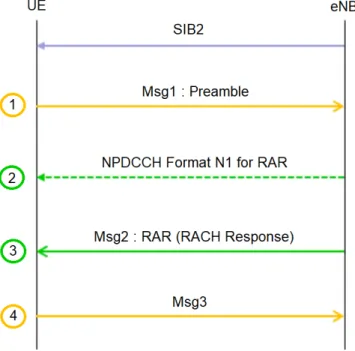
5.3 RAR Procedure . . . 44
5.4 NPUSCH Format 1 UE procedure . . . 46
6 NB-IoT MATLAB Modeling and USRP Co-Simulation 55
6.1 Introduction . . . 55
6.2 MATLAB Implementation . . . 56
6.2.1 Notation . . . 56
6.2.2 NPUSCH Format 1 simulation . . . 56
6.2.2.1 Transmitter Implementation . . . 56
6.2.2.2 Channel Implementation . . . 59
6.2.2.3 Receiver Implementation . . . 61
6.2.3 NPUSCH Format 2 Simulation . . . 63
6.2.3.1 Transmitter Implementation . . . 63 6.2.3.2 Channel Implementation . . . 64 6.2.3.3 Receiver Implementation . . . 64 6.2.4 NPRACH Simulation . . . 65 6.2.4.1 Transmitter Implementation . . . 66 6.2.4.2 Channel Implementation . . . 66 6.2.4.3 Receiver Implementation . . . 66 6.3 USRP Co-simulation . . . 67 6.3.1 USRP Implementation . . . 67
6.3.2 Carrier Frequency Offset . . . 69
6.3.3 Symbol Time Offset . . . 70
7 Results 71 7.1 Simulation Results . . . 71
7.1.1 NPUSCH Format 1 Simulation Results . . . 71
7.1.1.1 Transmitter - Constellations and Eye Diagram . . . 73
7.1.1.2 AWGN Channel Model - Constellations and Eye Diagrams . 74 7.1.1.3 Fading Channel Models - Constellations and Eye Diagrams . 77 7.1.1.4 Fading Channel with AWGN - Constellations and Eye Diagrams 81 7.1.1.5 BER . . . 83
7.1.1.6 Magnitude Spectrum . . . 87
7.1.1.7 PAPR . . . 88
7.1.2 NPUSCH Format 2 Simulation Results . . . 88
7.1.2.1 Constellation - Transmitter . . . 90
7.1.2.2 Fading Channel with AWGN - Constellations . . . 90
7.1.2.3 BER . . . 90
7.1.2.4 Repetitions Test, PAPR and Magnitude Spectrum . . . 91
7.1.3 NPRACH Simulation Results . . . 92
7.1.3.1 Constellation . . . 92
7.1.3.2 Correlation . . . 93
7.2 USRP Co-simulation Results . . . 94
7.2.1 NPUSCH Format 1 . . . 95
7.2.1.1 Constellation and Eye Diagram - Transmitter . . . 95
7.2.1.2 Constellation and Eye Diagram - Receiver . . . 95
7.2.1.3 BER . . . 95
7.2.1.4 Magnitude Spectrum . . . 97
7.2.2 NPUSCH Format 2 . . . 98
8 Conclusions and Future Work 99
8.1 Conclusions . . . 99
8.2 Future Work . . . 99
Bibliography 101 A User Guide 105 A.1 NPUSCH Format 1/2 Simulation . . . 105
A.2 NPRACH Simulation . . . 107
A.3 BER Performance Simulation . . . 108
A.4 USRP Co-simulation . . . 109
B Reference Sequence Test 110 B.1 NPUSCH Format 1 . . . 110
List of Figures
1.1 Projected number of IoT devices by year [SWH17]. . . 1
1.2 Uplink and downlink transmission. . . 3
2.1 Examples of NB-IoT deployments: stand-alone, LTE in-band and LTE guard-band [YPEWR17]. . . 7
2.2 Antenna configuration for SISO and SIMO systems [LGV14]. . . 8
2.3 Frame structure type 1 [GZAM10]. . . 9
2.4 Guard time for half-duplex FDD type B duplex scheme [DPS16]. . . 10
2.5 Structure of the uplink resource grid [GZAM10]. . . 11
2.6 Comparison of OFDMA and SC-FDMA multiple access technologies [Not09]. 12 2.7 Uplink shared channel mapping [GZAM10]. . . 14
2.8 Random access channel mapping [GZAM10]. . . 14
2.9 Uplink control information mapping [GZAM10]. . . 15
3.1 Block diagram of the NB-IoT UL-SCH transmitter [GZAM10]. . . 17
3.2 CRC addition example [Blo17a]. . . 18
3.3 Turbo encoder block diagram (dotted lines apply for trellis termination only) [3GP17a]. . . 19
3.4 Scheme of the convolutional encoder and corresponding trellis diagram for the encoding bits [Li09]. . . 20
3.5 Scheme of the convolutional encoder and corresponding trellis diagram for the termination bits [Li09]. . . 21
3.6 Rate matching block diagram [3GP17a]. . . 22
3.7 Virtual circular buffer with the three interleaved encoded bit streams. The arrows represent the starting point for the bit selection depending on the rvidx value [SP16]. . . 23
3.8 QPSK modulation mapping. . . 25
3.9 BPSK modulation mapping. . . 26
3.10 SC-FDMA modulation schematic [DT17]. . . 26
3.11 Resource mapping using a resource unit with six available subcarriers. . . 27
3.12 Cyclic prefix addition [DT17]. . . 27
3.13 Block diagram of the NB-IoT UCI transmitter [GZAM10]. . . 28
3.14 Resource elements used for DMRS in NPUSCH format 1. On the left, is an example when ∆f is 3.75kHz. On the right, is an example with 6 subcarriers and ∆f = 15kHz [Roh16]. . . 30
3.15 Resource elements used for demodulation reference signals in NPUSCH format
2. In this format, the RU only occupies one subcarrier [Roh16]. . . 30
3.16 Preamble symbol group [Roh16]. . . 30
3.17 NB-IoT PRACH design [LAW16]. . . 31
4.1 Block diagram of the NB-IoT UL-SCH receiver [GZAM10]. . . 33
4.2 SC-FDMA demodulation schematic [DT17]. . . 34
4.3 Rate dematching block diagram. . . 37
4.4 Scheme of the NB-IoT turbo decoder [Li09]. . . 38
4.5 CRC check example [Blo17a]. . . 40
4.6 Block diagram of the NB-IoT UCI receiver [GZAM10]. . . 40
5.1 Overall RAR procedure. SIB2 transmission is required before the RAR proce-dure itself. . . 44
5.2 Contents of DCI format N1 when is used for scheduling NPRACH [DT17]. . . 45
5.3 Overall NPUSCH format 1 UE procedure. . . 46
5.4 Contents of DCI format N0 [DT17]. . . 47
5.5 Allocated subcarriers as indicated by nsc [DT17]. . . 48
5.6 Example of an arrangement for NPUSCH transmission with 8 repetitions. For the case of no repetitions, the slot sequence shown in (b) would be transmitted [Roh16]. . . 49
5.7 Overall NPUSCH format 2 UE procedure. . . 51
5.8 Contents of DCI format N1 when used for scheduling NPDSCH [DT17]. . . . 52
6.1 Block diagrams of the MATLAB implemented simulations. . . 57
6.2 Simplified model of the USRP modulation/demodulation process [oE17]. . . . 68
7.1 MATLAB implemented chain schematic for NPUSCH format 1. Measures of constellations and eye diagrams happen on points a) and b). . . 72
7.2 Transmitter constellations. . . 73
7.3 Transmitter eye diagram - BPSK/QPSK have equal eye diagrams. . . 74
7.4 QPSK constellation for AWGN channel when Eb/N0 is 8dB. . . 75
7.5 QPSK eye diagram for AWGN channel when Eb/N0 is 8dB. . . 75
7.6 QPSK constellation for AWGN channel when Eb/N0 is 0dB. . . 76
7.7 QPSK eye diagram for AWGN channel when Eb/N0 is 0dB. . . 76
7.8 QPSK constellation for EPA channel model. . . 77
7.9 QPSK eye diagram for EPA channel model. . . 78
7.10 QPSK constellation for EVA channel model. . . 78
7.11 QPSK eye diagram for EVA channel model. . . 79
7.12 QPSK constellation for ETU channel model. . . 79
7.13 QPSK eye diagram for ETU channel model. . . 80
7.14 QPSK constellation for EVA channel model with AWGN (Eb/N0 is 8dB). . . 81
7.15 QPSK eyediagram for EVA channel model with AWGN (Eb/N0 is 8dB). . . . 82
7.16 BPSK constellation for EVA channel model with AWGN (Eb/N0 is 8dB) - no equalizer is implemented on the left figure and ZF equalizer is used on the right figure. . . 82
7.17 BPSK eye diagram for EVA channel model with AWGN (Eb/N0 is 8dB) - no equalizer is implemented on the left figure and ZF equalizer is used on the right
figure. . . 83
7.18 BER performance results for an AWGN channel. . . 84
7.19 BER performance results for EPA, EVA and ETU channel fading models with added Additive White Gaussian Noise (AWGN). Equalizer and turbo coding are used. . . 85
7.20 BER performance results for a EVA channel model with AWGN. . . 86
7.21 BER performance results for each NRep value. . . 87
7.22 Transmitted and received magnitude spectrums. . . 87
7.23 SC-FDMA PAPR. . . 88
7.24 MATLAB implemented chain schematic for NPUSCH format 2. Measures of constellations and eye diagrams happen on points a) and b). . . 89
7.25 BPSK constellation for EVA channel model with AWGN (Eb/N0 is 8dB). . . 90
7.26 BPSK constellation for EVA channel model with AWGN (Eb/N0 is 12dB). . . 91
7.27 BER performance results for a EVA channel model with AWGN, with and without equalizer. . . 91
7.28 MATLAB implemented chain schematic for NPRACH. Measures of constella-tions and cross-correlaconstella-tions happen on points a) and b). . . 92
7.29 NPRACH transmitted and received constellations. . . 93
7.30 Auto-correlation of the transmitted preamble and cross-correlation between the expected and received preamble. . . 93
7.31 Implemented chain schematic for a co-simulation environment. Measures of constellations and eye diagrams happen on points a) and b). . . 94
7.32 QPSK and BPSK received constellations for NPUSCH format 1. . . 96
7.33 QPSK and BPSK received eye diagrams for NPUSCH format 1. . . 96
7.34 Magnitude spectrum of the transmitted and received signals. . . 97
7.35 BPSK received constellation for NPUSCH format 2. . . 98
A.1 User input parameters list for NPUSCH format 1 and 2 simulation. . . 105
A.2 Command window output for NPUSCH format 1. . . 106
A.3 Command window output for NPUSCH format 2. . . 107
A.4 User input parameters list for NPRACH simulation. . . 108
A.5 User input parameters list for BER simulation. . . 108
List of Tables
1.1 NB-IoT and LoRa comparison [SWH17]. . . 2
2.1 Number of subcarriers, frame length, subframe length and slot length values depending on ∆f . . . 8
2.2 RU duration for NPUSCH format 1. . . 13
2.3 RU duration for NPUSCH format 2. . . 13
3.1 Polynomial used on CRC addition in NB-IoT. . . 18
3.2 Inter-column permutation pattern for sub-block interleaver. . . 22
3.3 Relationship between the modulation scheme and Qm. . . 25
3.4 HARQ-ACK codewords. . . 28
4.1 QPSK modulation demapping. . . 35
4.2 BPSK modulation demapping. . . 35
4.3 Descrambling operation between the Gold sequence c(n) and the received bits ˜b(n). . . . 35
4.4 HARQ-ACK decoding. . . 41
5.1 NRU obtained according to IRU value. . . 47
5.2 Values of allocated subcarriers nsc depending on the subcarrier indicator Isc. 47 5.3 Qm and IT BS obtained according to the IM CS value. . . 48
5.4 NRep obtained according to the IRep value. . . 48
5.5 TBS obtained according to IT BS and IRU values. . . 50
5.6 NPUSCH format 2 allocated subcarrier when ∆f = 3.75kHz. . . 52
5.7 NPUSCH format 2 allocated subcarrier when ∆f = 15kHz. . . 53
6.1 Function GetParametersF1() description. . . 58
6.2 Function CodingProcessF1() description. . . 58
6.3 Function Generate DMRSF1() description. . . 58
6.4 Function ModulationProcess() description. . . 59
6.5 EPA Delay Profile. . . 60
6.6 EVA Delay Profile . . . 60
6.7 ETU Delay Profile. . . 60
6.8 Function ChannelSim() description. . . 61
6.9 Function ChannelEstF1() description. . . 61
6.10 Function DemodulationProcessF1() description. . . 62
6.12 Function DataDispF1() description. . . 62 6.13 Function GetParametersF2() description. . . 63 6.14 Function CodingProceduresF2() description. . . 63 6.15 Function Generate DMRSF2() description. . . 63 6.16 Function ModulationProcessF2() description. . . 64 6.17 Function ChannelEstF2() description. . . 65 6.18 Function DemodulationProcessF2() description. . . 65 6.19 Function DecodingProcessF2() description. . . 65 6.20 Function DataDispF2() description. . . 66 6.21 Function NprachGen() description. . . 66 6.22 Function NprachDetect() description. . . 66 6.23 Function FrequencyOffset() description. . . 69 6.24 Function TimeOffset() description. . . 70 7.1 Variation of the co-simulation BER with the distance between USRPs. . . 97 7.2 Variation of the co-simulation BER with IRep. . . 97
List of Acronyms
3GPP 3rd Generation Partnership Project . . . 2 ACK/NACK Acknowledgement/Negative-Acknowledgement . . . 51 ADC Analog-to-Digital Converter . . . 67 AWGN Additive White Gaussian Noise . . . vii BER Bit Error Ratio . . . 70 BPSK Binary Phase-Shift Keying . . . 11 CAZAC Constant Amplitude, Zero AutoCorrelation . . . 31 CCDF Complementary Cumulative Distribution Function . . . 88 CFO Carrier Frequency Offset . . . 4 CP Cyclic Prefix . . . 10 CRC Cyclic Redundancy Check . . . 17 DCI Downlink Control Information . . . 45 DFT Discrete Fourier Transform . . . 12 DL-SCH Downlink Shared Channel . . . 46 DMRS Demodulation Reference Signal . . . 4 DSP Digital Signal Processing . . . 67 eNodeB Evolved Node B . . . 2 EPA Extended Pedestrian A . . . 59 ETU Extended Typical Urban . . . 59 EVA Extended Vehicular A . . . 59 FDD Frequency Division Duplex . . . 9 FFT Fast Fourier Transform . . . 9 FPGA Field-Programmable Gate Array . . . 67 FSM Finite State Machine . . . 20 GSM Global System for Mobile communications . . . 7 HARQ-ACK HARQ Acknowledgement . . . 28 IDFT Inverse Discrete Fourier Transform . . . 34 IFFT Inverse Fast Fourier Transform. . . .12
IoT Internet of Things . . . 1 ISI Inter Symbol Interference . . . 27 LoRa Long Range Radio . . . 2 LPWAN Low Power Wide Area Networks . . . 1 LTE Long Term Evolution . . . 3 MAC Media Access Control . . . 13 MAP Maximum A Posteriori . . . 38 MATLAB MATrix LABoratory . . . 3 MMSE Minimum Mean-Squared Error . . . 99 MSb Most Significant bit . . . 45 NB-IoT Narrowband Internet of Things . . . 2 NPDCCH Narrowband Physical Downlink Control Channel . . . 43 NPDSCH Narrowband Physical Downlink Shared Channel . . . 43 NPRACH Narrowband Physical Random Access Channel . . . 13 NPSS Narrowband Primary Synchronization Signal . . . 44 NPUSCH Narrowband Physical Uplink Shared Channel . . . 12 NSSS Narrowband Secondary Synchronization Signal . . . 44 OFDMA Orthogonal Frequency Division Multiple Access . . . 11 PAPR Peak-to-Average Power Ratio . . . 12 PRACH Physical Random Access Channel . . . 17 PUCCH Physical Uplink Control Channel . . . 14 QoS Quality of Service . . . 2 QPSK Quadrature Phase-Shift Keying . . . 11 RACH Random Access Channel . . . 4 RAR Random Access Response . . . 14 RF Radio Frequency . . . 3 RLC Radio Link Control . . . 13 RNTI Radio Network Temporary Identifier . . . 46 RSC Recursive Systematic Convolutional . . . 19 RU Resource Unit . . . 4 SC-FDMA Single-Carrier Frequency-Division Multiple Access . . . 9 SDR Software Defined Radio . . . 67 SIB System Information Block . . . 44 SIMO Single-Input and Multiple-Output . . . 8 SINR Signal-to-Interference-plus-Noise Ratio . . . 25 SISO Single-Input and Single-Output . . . 8
SMA SubMiniature version A . . . 67 SNR Signal-to-Noise Ratio . . . 84 SOVA Soft Output Viterbi Algorithm . . . 38 STO Symbol Time Offset. . . .4 TBS Transport Block Size . . . 13 TDD Time Division Duplex . . . 9 UCI Uplink Control Information . . . 4 UE User Equipment . . . 2 UHD Universal Hardware Driver . . . 68 UL-SCH Uplink Shared Channel . . . 4 USB Universal Serial Bus . . . 67 USRP Universal Software Radio Peripheral . . . 4 ZC Zadoff-Chu . . . 31 ZF Zero Forcing . . . 41
List of Symbols
∆f subcarrier spacing . . . 8 E total number of bits available for the transmission of one transport block . . . 23 IDelay scheduling delay indication field . . . 45 IM CS modulation and coding scheme indication field . . . 45 IRep repetition number indication field . . . 45 IRU resource assignment indication field . . . 46 Isc subcarrier indication field . . . 45 ISF resource assignment indicator . . . 51 IT BS transport block size indication field . . . 47 MidenticalN P U SCH number of repetitions of grouped slots . . . 49 MRepN P U SCH scheduled number of repetitions of a NPUSCH transmission . . . 49 nf frame number . . . 24 NRep total number of repetitions . . . 47 NRU total number of resource units . . . 12 ns slot number . . . 24 nsc number of subcarriers allocated to NPUSCH . . . 47 Nslots number of grouped slots . . . 49 NRepAN ACK/NACK number of repetitions . . . 52 NIDN cell narrowband physical layer cell identity . . . 43 NrepN P RACH number of NPRACH repetitions per attempt . . . 31 NscN P RACH number of subcarriers allocated to NPRACH . . . 44 Nscof f setN P RACH frequency location of the first subcarrier allocated to NPRACH . . . 44 NscRU number of consecutive subcarriers in a resource unit . . . 12 NU L
sc number of uplink subcarriers . . . 8 NslotsU L number of uplink slots in each resource unit . . . 12 NsymbolsU L number of symbols in a slot . . . 12 Qm modulation order . . . 22 rvdci redundancy version indication field . . . 46
rvidx transmission redundancy version . . . 23 ru value of the demodulation reference signals . . . 29
Chapter 1
Introduction
1.1
Framework
Over the last years the Internet of Things (IoT) market has grown exponentially, becom-ing one of the most active areas of technology development. It is constantly changbecom-ing and adapting, being the focus of many research and investment initiatives.
The IoT refers to a network of interconnected devices such as sensors/actuators, outfitted with data-collecting technologies in order to communicate with one another. This should enable seamless integration of potentially any object into the Internet, thus allowing for new forms of interactions between human beings and devices, or directly between devices [CVZZ16].
Figure 1.1: Projected number of IoT devices by year [SWH17].
According to Figure 1.1, by 2020, more than twenty billion devices will be connected through wireless communications. Low Power Wide Area Networks (LPWAN) technologies have become popular, in order to fulfill the IoT market’s rapid growth. Their shared features are wide coverage, low bandwidth, small data sizes and long battery life. LPWAN proto-cols are divided in two groups: the ones that use licensed spectrum and the ones that use
unlicensed spectrum. A comparison between two of the leading technologies in each group, 3rd Generation Partnership Project (3GPP) Narrowband Internet of Things (NB-IoT) and Semtech Long Range Radio (LoRa), is presented in Table 1.1.
Table 1.1: NB-IoT and LoRa comparison [SWH17].
LoRa NB-IoT
Quality of Service
LoRa uses an unlicensed spectrum and cannot offer the same QoS
as NB-IoT.
NB-IoT uses a licensed spectrum and its time slotted synchronous
protocol is optimal for QoS. Cost
Spectrum cost is free. Gateways are cheap when compared with
NB-IoT base stations.
Spectrum cost is very high. Base stations are more expensive
than the LoRa equivalent.
Battery life
LoRa devices can sleep for as little or as long as the application desires, since it is an asynchronous protocol.
In NB-IoT, because of infrequent but regular synchronization, the device consumes additional battery
energy.
Latency
LoRa has less energy demands, which leads to a higher latency
and lower data rate.
Although the energy demands are bigger in NB-IoT, this
leads to a lower latency and higher data rate. Network
coverage
LoRa can cover a whole city using one gateway.
The deployment of NB-IoT is limited to
4G/LTE base stations.
Range <15 km <35 km
Deployment model
LoRa components are production-ready now.
Requires a software upgrade for the base stations.
Standard Closed Open
In summary, it is shown that LoRa has advantages in terms of battery lifetime and cost, and NB-IoT has benefits regarding Quality of Service (QoS), latency and reliability.
Although both have qualities, there are two key factors worth mentioning. First, LoRa is already fully tested and functional, with modules easily available. Meanwhile, NB-IoT is still to be implemented, requiring a software upgrade in the network’s Evolved Node B (eN-odeB). Thus, it requires a proof of concept before its hardware implementation, making it the ideal choice for a behavioral model simulation. Secondly, NB-IoT is an open standard, mean-ing there is enough information available to simulate and analyze this protocol in different platforms. Therefore, NB-IoT will be the main focus of this master thesis.
1.1.1 NB-IoT Overview
This subsection briefly summarizes the NB-IoT uplink and downlink transmission direc-tions, introducing concepts required to further understanding the protocol. Figure 1.2 depicts a transmission between two User Equipments (UEs) and an eNodeB in both directions (uplink and downlink).
Figure 1.2: Uplink and downlink transmission.
Generally, uplink means the UE transmits a signal to the eNodeB, and downlink corre-sponds to a transmission from the eNodeB to the UE.
Each transmission mode requires a huge amount of signal processing, being quite com-plex. Therefore, two different dissertations were proposed, one for the uplink and one for the downlink, with the uplink transmission being the main focus of this dissertation.
1.2
Motivation
Newly introduced systems, modulation techniques and protocols usually use behavioral models simulated in MATrix LABoratory (MATLAB) to test their functionalities. Imple-mentations without the concern for real time data processing, clock cycles and latency are essential, as they provide a simplified analysis which can be used as a proof of concept. NB-IoT is a new protocol, with several differences when compared to Long Term Evolution (LTE). Therefore, an analysis and implementation of its data generation algorithms is necessary. The simulation results may also be used as a reference for hardware performance tests. Further-more, it can be integrated in the MATLAB LTE toolbox, which up to this moment doesn’t have any NB-IoT uplink functionalities.
A big advantage of these systems is their portability. Besides tests in a simulation envi-ronment, it is possible to analyze and verify the transmitter/receiver chain in a co-simulation environment, with the signal being generated/captured using two Radio Frequency (RF) front-ends. This decreases the required amount of time for the development process, reducing the number of bugs that will be found.
1.3
Objectives
The goals of this master thesis are the following:
• Model and simulate the physical layer of a NB-IoT uplink transmitter in MATLAB. This includes all the physical channels and signals with their respective coding and modulation.
• Model and simulate the physical layer of a NB-IoT uplink receiver in MATLAB. This includes the decoding and demodulation of all uplink physical channels and signals. • Simulate different channel models to test how the generated transmitted signal is
af-fected. Implement and validate a channel estimator and equalizer in order to mitigate those effects.
• Choose a RF front-end compatible with MATLAB, to send and capture signals based on a co-simulation environment. Implement functions that allow for Carrier Frequency Offset (CFO) and Symbol Time Offset (STO) estimation and correction.
1.4
Contributions
The main contributions of this master thesis include:
• The design of a behavioral model for NB-IoT physical layer in MATLAB, including all channels and signals.
• A performance evaluation using different channel models in a simulation environment and two Universal Software Radio Peripherals (USRPs) as RF front-ends, for a closer to reality environment.
1.5
Thesis Structure
This thesis is divided into 8 chapters:
• Chapter 1 - “Introduction”: contains a brief description about IoT and the overall motivation behind the development and creation of a NB-IoT uplink transceiver. It also briefly summarizes the main goals to be achieved with this master thesis.
• Chapter 2 - “NB-IoT General Concepts”: presents an overview on the basics of a NB-IoT system, its deployments options, frame structure and duplex arrangements. It’s also explained, in detail, the new time-frequency grid and a new concept not present in LTE - Resource Units (RUs). To finish, an overview of all physical channels and signals is done.
• Chapter 3 - “NB-IoT Uplink Transmitter”: explains the Uplink Shared Channel (UL-SCH) coding (CRC addition, turbo coding and rate matching) and the Uplink Control Information (UCI) channel coding. Furthermore, their modulation (scrambling, modulation mapper and SC-FDMA modulation) is explained in detail. Afterwards, the Random Access Channel (RACH) preamble generation is described, as is the creation of Demodulation Reference Signal (DMRS).
• Chapter 4 - “NB-IoT Uplink Receiver”: explains the UL-SCH decoding (CRC removal, turbo decoding and rate dematching) and the UCI channel decoding. Fur-thermore, their demodulation (descrambling, modulation demapping and SC-FDMA demodulation) is explained in detail. Afterwards, the RACH preamble detection is described. Channel estimation and equalization based on the received DMRS is also clarified.
• Chapter 5 - “NB-IoT Physical Layer Procedures”: explains the required proce-dures to send data in each specific channel. It is emphasized the scheduling order and how necessary parameters are obtained, in order to generate a transport block to be sent over any channel.
• Chapter 6 - “MATLAB Simulation and USRP Implementation”: presents block diagrams with the MATLAB simulation and the USRP co-simulation work flow. Its main functions are explained in detail, showing their input and output parameters, with a explanation of their main purpose. It’s also justified the reason why MATLAB was chosen.
• Chapter 7 - “Performance Results”: shows all the results, simulated and measured, throughout this work. It includes constellations, eye diagrams and BER performances. They are compared and discussed to offer a better perspective of the overall developed work.
• Chapter 8 - “Conclusion and Future Work”: marks the end of this thesis with a summary of the developed work and presents some propositions for possible future works.
The following appendixes were included:
• Appendix A - “User Guide”: provides a small user guide on how to run the im-plemented simulations. Furthermore, a step by step explanation on how to test the co-simulation environment is provided.
• Appendix B - “Reference Sequence Test”: shows what happens when a know sequence is imposed in the beginning of the simulation, contributing with a reference sequence test in each main point of the transmitter and receiver chain for both NPUSCH format 1 and 2.
Chapter 2
NB-IoT General Concepts
This chapter provides introductory concepts, necessary to understand the NB-IoT physical layer.
2.1
Deployment Options
NB-IoT can operate in three different modes [Roh16]:
• Stand alone operation, where a possible option is the replacement of the Global System for Mobile communications (GSM) carriers by a NB-IoT cell. Considering NB-IoT has a bandwidth of 180kHz (discussed in section 2.3) and GSM has a bandwidth of 200 kHz, there is a guard interval of 10 kHz on both sides of the spectrum.
• Guard band operation utilizing resource blocks within a LTE carrier’s guard-band. • In-band operation utilizing one resource block in the LTE carrier.
These different deployment scenarios are illustrated in Figure 2.1.
Figure 2.1: Examples of NB-IoT deployments: stand-alone, LTE in-band and LTE guard-band [YPEWR17].
2.2
Antenna Selection
Up to this moment, NB-IoT uplink supports only one transmission mode, which consists on a transport block transmission using a single physical antenna. A wireless communications system in which one antenna is used at the source (transmitter) and one antenna is used at the destination (receiver) is called Single-Input and Single-Output (SISO), being the simplest antenna technology - Figure 2.2a.
In some environments, SISO systems are vulnerable to problems caused by multipath effects. When the waves have obstructions in their path, they are scattered and take different paths to reach the receiver. Each scattered signal arrives at different times, which causes problems, such as fading. In order to minimize them, it is possible to have more than one antenna at the receiver (eNodeB). A system in which one antenna is used at the source (transmitter) and two antennas are used at the destination (receiver) is called Single-Input and Multiple-Output (SIMO) - Figure 2.2b [Blo17b].
(a) Antenna configuration for SISO systems.
(b) Antenna configuration for SIMO systems.
Figure 2.2: Antenna configuration for SISO and SIMO systems [LGV14].
2.3
Subcarrier Spacing
In the uplink, both 3.75kHz and 15kHz subcarrier spacing (∆f ) are supported. Observing Table 2.1, it’s possible to conclude that when ∆f is equal to 15kHz the number of uplink subcarriers (NscU L) is 12 and when ∆f equals 3.75kHz the NscU Lis 48. Thus, the bandwith for NB-IoT is easily obtained multiplying ∆f by NscU L - 15kHz × 12 = 3.75kHz × 48 = 180kHz. Table 2.1: Number of subcarriers, frame length, subframe length and slot length values depending on ∆f .
Parameters ∆f = 15kHz ∆f = 3.75kHz
Number of subcarriers 12 48
Radio frame length 10ms 40ms
Subframe length 1ms 4ms
Slot length 0.5ms 2ms
If ∆f is equal to 15kHz, the radio frame has a length of Tf = 10ms, with subframes of length Tsf = 1ms and slots of length Tslot = 0.5ms. The symbol time is 1/∆f ≈ 66.7µs. If ∆f has the value of 3.75kHz, the radio frame has a length of Tf = 40ms, with subframes of length Tsf = 4ms and slots of length Tslot= 2ms. The symbol time is 1/∆f ≈ 266, 7µs.
2.4
Frame Structure
In LTE, two types of frame structures are supported, selected according to the duplex mode: Time Division Duplex (TDD) or Frequency Division Duplex (FDD). Since in NB-IoT, only FDD mode is supported (discussed in section 2.5), frame structure type 1 is used.
2.4.1 Frame Structure Type 1
In the time domain, NB-IoT transmissions are organized into radio frames, each of which is divided into ten equal subframes, as illustrated in Figure 2.3. Each subframe consists of two equal slots, with each slot consisting of seven symbols, including cyclic prefix. Each symbol is Single-Carrier Frequency-Division Multiple Access (SC-FDMA) modulated - discussed in section 2.7.1.
Figure 2.3: Frame structure type 1 [GZAM10].
To provide consistent and exact timing definitions, different time intervals within the NB-IoT specifications are defined as multiples of a basic time unit T s = 1/(15000 × 128)s when ∆f = 15kHz or T s = 1/(3750 × 512)s when ∆f = 3.75kHz. The basic time unit T s can thus be seen as the sampling time of a transmitter/receiver with a Fast Fourier Transform (FFT) size equal to 128 when ∆f = 15kHz or 512 when ∆f = 3.75kHz.
2.5
Duplex Arrangements
Although in LTE both TDD and FDD are supported (providing spectrum flexibility), in NB-IoT only FDD half-duplex type B mode is supported.
2.5.1 Frequency-Division Duplex
In case of FDD operation, uplink and downlink use different carrier frequencies, denoted fU L and fDL. In each frame, there are ten uplink subframes and ten downlink subframes, and uplink and downlink can happen simultaneously. Isolation between both transmissions is obtained using duplex filters. In certain frequency bands with a very narrow duplex gap, it is challenging to design the duplex filters. In this case, a device only supports half-duplex operation. Half-duplex operation requires a guard period where the device can switch between transmission and reception.
LTE supports two ways of providing the necessary guard period [DPS16]:
• Half-duplex type A, where guard time for the switch is handled by setting the necessary amount of timing advance in the devices.
• Half-duplex type B, where a whole subframe is used as guard between reception and transmission, with an oscillator that is retuned between uplink and downlink frequencies. Thus, for NB-IoT, uplink and downlink are separated in frequency and the UE either receives or transmits, but never does both simultaneously. In addition, between every switch from uplink to downlink or vice-versa there is at least one guard subframe in between, allowing the UE to switch its transmitter to receiver chain and vice-versa (Figure 2.4). This duplex scheme requires less complex hardware, allowing a lower-cost implementation, ideal for IoT applications.
Figure 2.4: Guard time for half-duplex FDD type B duplex scheme [DPS16].
2.6
NB-IoT Time-Frequency Grid
This section describes the basic NB-IoT time-frequency transmission grid. Contrary to LTE where two Cyclic Prefix (CP) lengths are defined, NB-IoT only supports the normal CP length, corresponding to seven symbols per slot. Figure 2.5 depicts the resource grid for a single slot.
When ∆f is equal to 15kHz, the resource grid is equal to the one for LTE with normal CP, using only one resource block. When ∆f is equal to 3.75kHz, the resource grid for a slot has a different structure, since the NscU L is 48, instead of 12.
A resource element, which is the smallest physical resource in NB-IoT, is indicated in Figure 2.5 by one square. Furthermore, resource elements are grouped into a resource block. If ∆f = 15kHz, each resource block consists of 12 consecutive subcarriers in the frequency domain (NscU L = 12) and one 0.5ms slot in the time domain. Therefore, each resource block consists of 7 × 12 = 84 resource elements. If ∆f = 3.75kHz, each resource block consists of 48 consecutive subcarriers in the frequency domain (NscU L = 48) and one 2ms slot in the time domain. Each resource block thus consists of 7 × 48 = 336 resource elements. Each resource element in the resource grid is defined by the index pair (k, l) in a slot, where k = 0, ..., NscU L− 1 and l = 0, ..., NU L
symb− 1 are the indices in the frequency and time domain, respectively [DPS16].
Figure 2.5: Structure of the uplink resource grid [GZAM10].
2.7
Transmission Scheme
The NB-IoT uplink uses both multi-tone and single-tone transmissions. Multi-tone trans-mission uses ∆f = 15kHz, equal to LTE. While only the 12-tone format is supported by LTE UEs, 6-tone and 3-tone formats are added on NB-IoT UEs. Single-tone transmission is introduced for NB-IoT and supports two ∆f values, 15kHz and 3.75kHz [YPEWR17]. Uplink transmissions are based on SC-FDMA modulation.
2.7.1 SC-FDMA Overview
A graphical comparison of Orthogonal Frequency Division Multiple Access (OFDMA) (used in downlink) and SC-FDMA is shown in Figure 2.6. Although NB-IoT signals are allocated in 12 or 48 adjacent subcarriers (NscU L= 12 or 48), only four subcarriers are depicted. Even though uplink NB-IoT accepts both Binary Phase-Shift Keying (BPSK) and Quadrature Phase-Shift Keying (QPSK) modulation schemes, in this example, data is represented using QPSK modulation.
In the OFDMA example of Figure 2.6, in each symbol period, four QPSK symbols are inserted in parallel, one per subcarrier. After each symbol period, the CP is inserted and the next four symbols are transmitted. Although the CP is shown as a gap, it is actually a copy of
Figure 2.6: Comparison of OFDMA and SC-FDMA multiple access technologies [Not09].
the next symbol’s ending. To create the transmitted signal, an Inverse Fast Fourier Transform (IFFT) is performed on each subcarrier. Adding together many parallel narrowband QPSK waveforms creates an undesirably high Peak-to-Average Power Ratio (PAPR). In the uplink this effect would be particularly damaging, since it would drain the UE battery rapidly.
In the SC-FDMA example of Figure 2.6, the four QPSK data symbols are transmitted in series at four times the rate, with each data symbol occupying M × 15kHz bandwidth. Therefore, the SC-FDMA signal appears to be more like a single-carrier, with each data symbol being represented by one wide signal. SC-FDMA signal generation can be seen as a Discrete Fourier Transform (DFT)-precoded OFDMA, which spreads the information over all the subcarriers. After the DFT, all the other steps occur as in OFDMA.
Detailed information about QPSK and BPSK modulation can be found on sub-subsection 3.1.2.2. More about SC-FDMA signal generation is presented in sub-subsection 3.1.2.3.
2.8
Resource Units
The smallest unit to map a transport block is the RU. A RU is defined as the number of uplink slots in each resource unit (NslotsU L ) multiplied by the number of consecutive subcarriers in a resource unit (NscRU), while in the frequency domain it is simply given by the total number of resource units (NRU) parameter. In NB-IoT, the number of symbols in a slot (NsymbolsU L ) is always 7.
The chosen RU depends on the Narrowband Physical Uplink Shared Channel (NPUSCH) format and ∆f . For NPUSCH format 1, there are five options presented in Table 2.2.
For NPUSCH format 2, the RU is always composed of one subcarrier with a length of four slots (Table 2.3).
Table 2.2: RU duration for NPUSCH format 1. ∆f NscRU NslotsU L RU duration 3.75kHz 1 16 32ms 15kHz 1 16 8ms 3 8 4ms 6 4 2ms 12 2 1ms
Table 2.3: RU duration for NPUSCH format 2. ∆f NscRU NslotsU L RU duration
3.75kHz 1 4 8ms
15kHz 1 4 2ms
2.9
NB-IoT Hierarchical Channel Structure and Reference
Signals
In this section, it is described the NB-IoT hierarchical channel structure. There are three different channel types: logical channels, transport channels, and physical channels. Logical channels carry data and signaling messages between the Media Access Control (MAC) and Radio Link Control (RLC) layers. Transport channels provide data characteristics between the MAC and physical layers, such as the modulation scheme. Physical channels are the implementation of transport channels over the radio interface, with a number of resource elements of the time-frequency grid carrying information from higher layers. Besides phys-ical channels, there is a signal embedded in the uplink physphys-ical layer, which does not carry information. This signal is called DMRS.
Figures 2.7 and 2.8 specify, respectively, the mapping of the UL-SCH and the RACH to their corresponding physical channels: NPUSCH format 1 and Narrowband Physical Random Access Channel (NPRACH). Figure 2.9 specifies the mapping of the UCI to its corresponding physical channel (NPUSCH format 2).
2.9.1 Uplink Physical Channels
Since this master thesis is mainly focused on the physical layer, an overview of the different physical channels and signal is done in this subsection.
2.9.1.1 NPUSCH Format 1 with DMRS
NPUSCH format 1 carries UL-SCH data, with maximum Transport Block Size (TBS) value of 1000 bits (much smaller than LTE). NPUSCH format 1 supports both multi-tone and single-tone transmissions using 7 symbols per slot (NsymbolsU L = 7), with the middle symbol being used to allocate the DMRS [Roh16, YPEWR17]. Further details regarding coding and modulation are discussed in section 3.1. The DMRS generation is detailed in section 3.3.
Figure 2.7: Uplink shared channel mapping [GZAM10].
Figure 2.8: Random access channel mapping [GZAM10].
2.9.1.2 NPUSCH Format 2 with DMRS
NPUSCH format 2 carries UCI, which is restricted to an acknowledgment of a downlink transmission. Even though in a downlink transmission it is configurable whether a transmis-sion shall be acknowledged, on uplink there is always an acknowledgment when a downlink transmission in received. NPUSCH format 2 also has 7 symbols per slot (NsymbolsU L = 7), but uses the middle three symbols to allocate the DMRS [Roh16, YPEWR17]. Further details re-garding coding and modulation are discussed in section 3.2. The DMRS generation is detailed in section 3.3.
2.9.1.3 NPRACH
NPRACH carries the random access preamble, whose signal generation is explained in section 3.4. It is used to iniciate the Random Access Response (RAR) procedure, when sent by the UE.
In summary, all data is sent over the NPUSCH, except for RACH transmission. This includes also the UCI, which is transmitted using a different format. Consequently, there is no equivalent to the Physical Uplink Control Channel (PUCCH) in LTE [Roh16,GZAM10].
Figure 2.9: Uplink control information mapping [GZAM10].
In this chapter, NB-IoT introductory concepts were explained. Deployment options, frame structure and duplex arrangements were summarized. The used time-frequency grid was depicted, and a new concept not used in LTE was introduced - RUs. A brief introduction to the available channels and signals was made. In the next chapter, the uplink transmitter architecture for all available physical channels will be explained in detail. Furthermore, the DMRS generation will be described.
Chapter 3
NB-IoT Uplink Transmitter
This chapter provides detailed information about the NB-IoT uplink physical layer trans-mitter. Section 3.1 describes the physical layer processing applied to the UL-SCH, section 3.2 explains the physical layer processing applied to the UCI, section 3.3 provides information about the DMRS and section 3.4 gives detailed information about the Physical Random Ac-cess Channel (PRACH) preamble generation. Knowledge about the transmitter proAc-cessing chain helps to fully understand the overall system operation implemented on MATLAB.
3.1
Uplink Shared Channel
This section describes the physical-layer processing applied to the UL-SCH and the sub-sequent mapping to the uplink physical resource in the form of the basic time-frequency grid. Figure 3.1 outlines the different steps of the UL-SCH physical layer processing.
Figure 3.1: Block diagram of the NB-IoT UL-SCH transmitter [GZAM10].
It is divided in coding and modulation procedures. The process called coding assists on the recovery of the transport block at the receiver side. Cyclic Redundancy Check (CRC) addition helps with error-detection, turbo coding adds redundancy to the data by adding two new data streams, which will be affected differently in case of a burst error. Finally, rate matching spreads out the occurrence of errors and punctures bits to fit the payload size. The process called modulation performs bit scrambling using a Gold sequence, modulates the
bits according to a specific modulation scheme and generates a baseband signal, where each symbol is based on SC-FDMA. Subsections 3.1.1 and 3.1.2 describe channel coding procedures and modulation procedures, respectively.
3.1.1 Channel Coding Processing
This subsection describes channel coding procedures. The process called channel coding transforms into codewords user data coming from transport blocks. This procedure, helps to correct/detect errors caused by distortion during transmission. The several coding procedures and their necessary steps are going to be explained in detail.
3.1.1.1 CRC Addition
CRC codes are an error-detection technique and the first step performed during the coding process. First, the transport block is divided by a generator polynomial. According to section 5.2.2.1 of [3GP17a], the 24A generator type is the baseline for the UL-SCH (Table 3.1).
Table 3.1: Polynomial used on CRC addition in NB-IoT. Type Generator polynomial
24A D24+ D23+ D18+ D17+ D14+ D11+ D10+ D7+ D6+ D5+ D4+ D3+ D + 1 Then, the previous division remainder is appended to the transport block. An example can be seen in Figure 3.2.
Figure 3.2: CRC addition example [Blo17a].
Let’s denote the polynomial generator by G and the transport block by D. In the example, G = 10011 and D = 1010101010. Since G is 5 bits long, then the remainder’s length (denoted by r) is G − 1 = 4, r = 4. D is shifted left by r bits and zeros will be inserted into those places. The new pattern will be denoted by D0 = 10101010100000. Now D0 is divided by G, using an “exclusive OR” operation. The remainder from the division, R, will be concatenated with the transport block D [Blo17a].
Considering the generator polynomial length is 25, the remainder added to the transport block will always have length equal to 24. Therefore, the output length (denoted by K) after the CRC addition will be K = T BS + 24.
3.1.1.2 Turbo Coding
This sub-subsection describes the turbo encoder and its components in detail. The turbo encoder is built using two identical Recursive Systematic Convolutional (RSC) encoders in parallel. The two RSC are separated by an interleaver, with its output being a permuted version of the input data. The purpose of the interleaver is to provide some degree of de-correlation among the inputs of each encoder. Therefore, in the event of a burst error, the two code streams are affected differently, allowing data to still be recovered. The structure of the turbo encoder is illustrated in Figure 3.3.
Figure 3.3: Turbo encoder block diagram (dotted lines apply for trellis termination only) [3GP17a].
At the beginning of encoding a message block, the RSC encoders are in a defined state of all-zeros. Three bit-streams are produced, the systematic signal (a), and one output of each encoder (parity signals c and d). The interleaved payload signal (b) is not transmitted, except during the trellis termination phase, as it can be easily reconstructed at the receiver side from a. After all the data bits have been encoded, trellis termination is performed bringing the encoders to an all-zeros state once again. To achieve this, the switches in Figure 3.3 are moved in the down position. The input, in this case, is shown by dashed lines. It takes three bits to force the final state back to all-zero state for each encoder. The output bit stream includes not only the tail bits corresponding to the upper encoder (e), but also the
tail bits corresponding to the lower encoder (f ). In addition to these six termination bits, six corresponding parity bits for the upper and lower encoder are also transmitted. Finally, all the bits are multiplexed into three data streams (d0, d1 and d2), that correspond to the input of the next step (rate-matching). Considering K the input length, the total length of the encoded bit sequence becomes 3K + 12, where each stream has outsize = K + 4 bits. The encoder code rate is calculated in equation 3.1.
r = K
3K + 12 (3.1)
However, for a large size of K, the loss in code rate due to tail bits is negligible and thus, with the code rate being approximately 1/3 [Imr13, Joo10].
RSC encoder: Each RSC encoder, has three memory bits forming an 8-state Finite State Machine (FSM). To understand the operation of the FSM, the state transition can be shown as a trellis diagram in Figure 3.4. Variable a is the input sequence and c is the output sequence. S1, S2 and S3 are the current state of the three memory bits in the encoder. S1+, S+2 and S3+ are the next state of the three memory bits. State1 to State8 correspond to the eight possible states. Figure 3.4 shows all the possible transitions for the encoding bits in a sequence. The first state in a transition is always the all-zeros one, corresponding to State1.
Figure 3.4: Scheme of the convolutional encoder and corresponding trellis diagram for the encoding bits [Li09].
The transition of the states and the decoding results can be expressed as the following equations:
S1+= ak⊕ S2⊕ S3 (3.2)
S2+= S1 (3.3)
S3+= S2 (3.4)
ck = S1+⊕ S1⊕ S3 (3.5)
Trellis termination: As mentioned above, this method involves three extra bits at the end of each sequence to force the encoder return to the all-zeros state. These extra bits are also sent to the decoder. In Figure 3.5, the state transition can be shown as a trellis diagram for the termination bits. Variable e is the input sequence and c is the output sequence. S1, S2 and S3 are the current state of the three memory bits in the encoder. S1+, S2+ and S3+ are the next state of the three memory bits. With this type of termination technique, the last state in the sequence is forced back to State1. This causes a number of limited transitions.
Figure 3.5: Scheme of the convolutional encoder and corresponding trellis diagram for the termination bits [Li09].
The transition of the states and the decoding results can be expressed as the following equations: S1+= 0 (3.6) S2+= S1 (3.7) S3+= S2 (3.8) ek= S2⊕ S3 (3.9) ck= 0 ⊕ s1⊕ S3 (3.10)
3.1.1.3 Rate Matching
The rate matching step forms a transport block that fits the payload size, calculated using the modulation order (Qm) and the total number of resource units (NRU). There are three steps that compose the rate matching process. Namely, sub-block interleaver, bit collection and bit selection (puncturing) (Figure 3.6).
Figure 3.6: Rate matching block diagram [3GP17a].
Interleaving is performed in order to spread out the occurrence of burst errors, which improves the overall performance of the decoder on the receiver side. Since the interleaving is performed separately for the systematic and parity bits obtained at the output of the turbo encoder, a bit collection stage is required to place the three bit streams in a specific order. Finally, the bit selection (puncturing) stage is needed in order to puncture some of the bits to create the required payload [Mat17c, GZAM10].
Sub-block interleaving: The inputs to the three sub-block interleavers correspond to each output stream from the turbo coding step. The interleaving is performed independently for each bit stream, using inter-column permutations.
Each input stream (with length D), is arranged into a matrix having C columns, C = 32. The number of rows, R, is determined in such a way that C × R >= D.
If D is not divisible by 32, it is necessary to add bits of nulls at the beginning of the matrix so it is completely full. The number of nulls, N , is N = C × R − D. The matrix size is K = N + D;
After, the matrix is rearranged using the inter-column permutation specified in Table 3.2. Table 3.2: Inter-column permutation pattern for sub-block interleaver.
Number of columns (C) Inter-column permutation pattern
32 <0, 16, 8, 24, 4, 20, 12, 28, 2, 18, 10, 26, 6, 22, 14, 30, 1, 17, 9, 25, 5, 21, 13, 29, 3, 19, 11, 27, 7, 23, 15, 31>
Bit collection: The bits collected from the interleaved streams are rearranged, forming a virtual circular buffer. The systematic bits are placed at the beginning, followed by the two interleaved parity streams, which are bit-by-bit interlaced, as shown in Figure 3.7. This
assures that an equal number of both versions of parity bits are transmitted. A virtual circular buffer is then formed and denoted by Wk, of size 3K bits [GZAM10].
Puncturer: The bit selection extracts consecutive bits from the circular buffer so that it fits into its assigned physical resource unit. To select the output bit sequence, its length should first be determined. Using the length value, denoted by E, bits are read from the virtual circular buffer. The starting point, denoted by k0 of the bit selection depends on the transmission redundancy version (rvidx).
The calculation of the total number of bits available for the transmission of one transport block (E ) and the starting point (k0) values goes as follows:
1) Calculate N c, which denotes the soft buffer size for the current transport block: N c = Kw = 3 × K (only for NB-IoT uplink).
2) Obtain G value, which is a parameter given by superior layers of the network and depends on the modulation order (Qm) and the total number of resource units (NRU).
3) For NB-IoT uplink, E = G.
4) Calculate k0, which is k0 = R × ((2 × dN c/(8 × R)e × rvidx) + 2), where rvidx is the redundancy version given to the UE by the eNodeB - subsection 5.1. For NB-IoT uplink, rvidx can have the value zero or two.
5) While bypassing the null bits added in the sub-block interleaver step, and using the output sequence length (E) and the starting point for the bit collection (k0), a codeword is obtained (Figure 3.7).
Figure 3.7: Virtual circular buffer with the three interleaved encoded bit streams. The arrows represent the starting point for the bit selection depending on the rvidx value [SP16].
After the rate matching process, a codeword is obtained. The coding procedure is finished.
3.1.2 Modulation Processing
This subsection describes the generic modulation procedures. In NB-IoT, modulation takes one codeword and converts it to a complex-valued baseband signal. As shown in Figure
3.1, the modulation processing consists of scrambling, modulation mapping and SC-FDMA modulation.
3.1.2.1 Scrambling
The first step on the modulation processing chain is the scrambling of coded data, which randomizes interference and avoids long sequences of equal bits.
The codeword obtained after the coding process (section 3.1.1) is scrambled according to equation 3.11:
˜b(i) = (b(i) + c(i)) mod 2, i = 0, 1, ... , Mb (3.11) where b(i) denotes the codeword of length Mb to be scrambled and c(i) denotes the pseudo-random Gold sequence described below.
Gold sequence: The Gold sequence is a result of modulo-2 binary addition of two sequences given by equations 3.12, 3.13 and 3.14:
x1(n + 31) = (x1(n + 3) + x1(n)) mod 2 (3.12)
x2(n + 31) = (x2(n + 3) + x2(n + 2) + x2(n + 1) + x2(n)) mod 2 (3.13)
c(n) = (x1(n + N c) + x2(n + N c)) mod 2 (3.14)
The value of N c is equal to 1600 and the length n is chosen as needed. Instead of the sequences being randomly generated, they are selected, making them only pseudo-random.
As can be seen in equations 3.12 and 3.13, there are 30 undefined values. The first sequence (x1) is always initialized with x1(0) = 1, x1(n) = 0, n = 1, 2, 3, ... , 30. The second sequence (x2) initialization is uniquely assigned depending on the Gold sequence application. For this specific application, x2 is initialized with cinit(equation 3.15) after its conversion to binary.
cinit= RNTI + nf mod 2.213+ bns/2c.29+ NIDN cell (3.15) where RNTI is the radio network temporary identifier and NIDN cell the narrowband physi-cal layer cell identifier. The frame number (nf) and the slot number (ns) vary with each transmission.
3.1.2.2 Modulation Mapper
The second step on the modulation processing chain consists on modulation mapping. For uplink, the supported data modulation schemes in NB-IoT include QPSK and BPSK, whose choice depends on the selected number of number of consecutive subcarriers in a resource unit (NscRU):
• For RUs with one subcarrier, BPSK and QPSK may be used. • For all other RUs, QPSK is applied.
The block of scrambled bits with length Mb is modulated into a block of complex-valued symbols, where Ms is the total number of modulated symbols. The relation between Ms and Mb is defined in equation 3.16.
Ms= Mb
Qm (3.16)
The modulation order (Qm) represents the number of bits in the modulation scheme constellation. The relationship between the modulation scheme used and Qm is represented on Table 3.3 [GZAM10].
Table 3.3: Relationship between the modulation scheme and Qm. Qm Modulation scheme
1 BPSK
2 QPSK
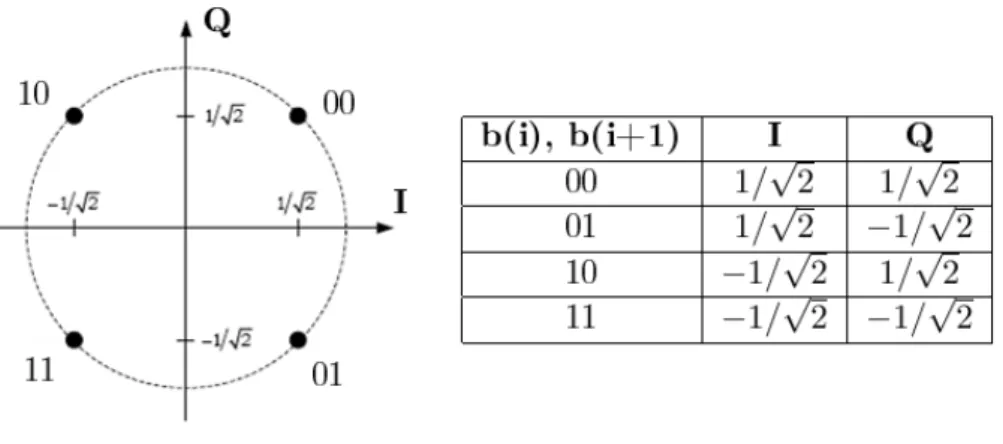
QPSK: It is a modulation technique that uses 2 bits per symbol. The modulation mapping is done according to Figure 3.8. There are four states (four possible combinations using two bits, 22 = 4). The theoretical bandwidth efficiency is two bits/second/Hz.
Figure 3.8: QPSK modulation mapping.
This modulation mapping uses Gray coding, which means that constellation points that are closer to each other differ in as few bits as possible. Therefore, fewer bits will be wrong, if the decoding is done incorrectly.
BPSK: It is a modulation technique that uses 1 bit per symbol. The modulation mapping is done according to Figure 3.9. There are two states (two possible combinations using one bit, 21 = 2). The theoretical bandwidth efficiency is one bit/second/Hz. BPSK is regarded as the most robust digital modulation technique and is used for long distance wireless communication.
Qm is selected based on the measured Signal-to-Interference-plus-Noise Ratio (SINR). Each modulation scheme has a threshold SINR. UEs closer to the eNodeB (with higher SINR values) use less robust modulation schemes. Meanwhile, UEs located further from the eNodeB (with lower SINR values) use a more robust modulation scheme. The eNodeB always selects the modulation order (Qm) to be used in uplink transmissions [Tel15].
Figure 3.9: BPSK modulation mapping.
3.1.2.3 SC-FDMA Modulation
Although NB-IoT uses OFDMA in the downlink, the uplink utilizes SC-FDMA. This is due to the fact that the overall value of PAPR is smaller then in OFDMA, for all modula-tion schemes. Therefore, it will consume considerably less energy, which is a fundamental characteristic for the UE operation.
SC-FDMA is divided in several steps, namely DFT precoding, resource mapping, padding addition, IFFT, resampling and CP addition. The schematic of the SC-FDMA modulation is represented in Figure 3.10.
Figure 3.10: SC-FDMA modulation schematic [DT17].
DFT precoding: SC-FDMA is a DFT coded OFDMA, which means that before go-ing through the standard OFDMA modulation, time domain data symbols are converted to frequency domain using a DFT [RBB17].
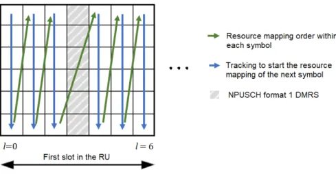
Resource Mapping: The resource mapping of each complex-valued symbol onto its corresponding resource element is done in increasing order, beginning with subcarriers and then SC-FDMA symbols, while bypassing DMRS. In Figure 3.11, the available resource unit has 6 subcarriers, therefore the resource mapping would go through 3 more slots - Table 2.2. Each slot is then repeated a certain number of times according to the parameter NRep -section 5.4.
Figure 3.11: Resource mapping using a resource unit with six available subcarriers.
Padding addition: A symbol consists of 12 or 48 resource elements, depending on ∆f . Each symbol is padded with additional zeros at each end, so it increases its size to the next power of two. This step has two goals. First, by being a power of two, the next step is simplified - IFFT. Secondly, if the DFT and IFFT had equal size, one would annul the other’s effect.
IFFT: The baseband signal is obtained using an IFFT operation. An IFFT transforms complex frequency domain symbols into a time domain signal.
Resample: Considering Fs = T1s ⇔ Fs = 1.92MHz, the time domain signal needs to be resampled, so a higher sampling rate of 1.92MHz is obtained. This is done, using interpolation, by a factor of eight.
CP addition: The term CP refers to the prefixing of each SC-FDMA symbol with a repetition of its end (Figure 3.12). The prefixing size varies with two factors: if it is the first symbol in the slot or not and according to the ∆f used.
The main objective of the CP addition is to be used as a guard interval, which eliminates the Inter Symbol Interference (ISI) [GZAM10, Roh16, DT17].
Figure 3.12: Cyclic prefix addition [DT17].
When the SC-FDMA modulation is terminated,the physical layer processing applied to the UL-SCH on the transmitter side is finished. The signal is in the baseband format.
3.2
Uplink Control Information
This section describes the physical-layer processing applied to the UCI and its mapping in the time-frequency grid. Figure 3.13 outlines the different steps of the UCI physical layer processing. It is divided in coding and modulation procedures, with subsections 3.2.1 and 3.2.2 describing channel coding procedures and modulation procedures, respectively.
Figure 3.13: Block diagram of the NB-IoT UCI transmitter [GZAM10].
3.2.1 Channel Coding Processing
This subsection describes the only channel coding step that transforms control information data into a codeword.
Control data is only sent on the NPUSCH format 2 when there is no UL-SCH data. The control data arrives to the channel coding unit in the form of an HARQ Acknowledgement (HARQ-ACK) indicator. The one bit information of HARQ-ACK is coded according to Table 3.4.
Table 3.4: HARQ-ACK codewords.
HARQ-ACK HARQ-ACK codeword
0 <0,0,0,0,0,0,0,0,0,0,0,0,0,0,0,0> 1 <1,1,1,1,1,1,1,1,1,1,1,1,1,1,1,1>
After this coding process, a codeword is obtained.
3.2.2 Modulation Processing
Modulation Processing steps are performed in exactly the same way as for the UL-SCH. Scrambling is done according to sub-subsection 3.1.2.1. Modulation mapping is done ac-cording to sub-subsection 3.1.2.2, always using BPSK as a modulation scheme. SC-FDMA modulation is done according to sub-subsection 3.1.2.3 always using a single subcarrier and, therefore, a single-tone transmission. When this is terminated, the physical layer processing applied to the UCI on the transmitter side is finished. The signal is in baseband format.
3.3
Demodulation Reference Signals
The value of the demodulation reference signals (ru) is transmitted on uplink resource units assigned to the UE and used for coherent demodulation/detection of data and control information at the eNodeB.
If the number of consecutive subcarriers in a resource unit (NscRU) is bigger than one, DMRS symbols are constructed from a base sequence multiplied by a phase factor defined in equation 3.17.
ru(n) = ej(ϕ(n)π/4+αn) (3.17)
where the value of ϕ(n) depends on the number of uplink subcarriers (NscU L) and the parameter u. If group hopping is not enabled, u is given by a higher layer parameter. If this parameter is undefined, then it is equal to a fixed value depending on NIDN cell and the NscRU.
If the NscRU equals one, DMRS symbols are constructed based on equations 3.18, 3.19 and 3.20. ¯ ru(n) = 1 √ 2(1 + j)(1 − 2c(n))w(n mod 16) (3.18) ru(n) = ¯ru(n), if NPUSCH format 1 (3.19) ru(3n + m) = ¯w(m) ¯ru(n), if NPUSCH format 2 (3.20) where c(n) is a Gold sequence initialized with cinit = 35 (paragraph 3.1.2.1) and w(n) depends on the variable u.
For NPUSCH format 2, ¯w(m) is a spreading orthogonal sequence.
3.3.1 Group Hopping Enabled
It is important to note that group hopping can only be enabled for NPUSCH format 1. If group hopping is enabled, u is defined by a group hopping pattern (fgh) and a sequence-shift pattern (fss). fgh is based on a Gold sequence (paragraph 3.1.2.1) initialized with cinit = b
NN cell ID
NRU seq
c. fss depends on the NIDN cell, NseqRU and a higher-layer parameter called ∆ss. NseqRU is a parameter that is based on the NscRU. If ∆ss is not defined, it assumes the value zero [3GP16, Roh16].
3.3.2 Resource Mapping of Demodulation Reference Signals
The DMRSs are transmitted in either one or three SC-FDMA symbols per slot, depending on the selected NPUSCH format.
For NPUSCH format 1 and ∆f = 3.75kHz, DMRS are transmitted in column number four (l = 4). For ∆f = 15kHz, they are transmitted in column number three (l = 3). These are the symbols indicated in red in Figure 3.14.
For NPUSCH format 2 and ∆f = 3.75kHz, DMRS are transmitted in columns number zero, one and two (l = 0, 1, 2). For ∆f = 15kHz, they are transmitted in columns number two, three and four (l = 2, 3, 4). These are the symbols indicated in red in Figure 3.15.
![Figure 2.1: Examples of NB-IoT deployments: stand-alone, LTE in-band and LTE guard- guard-band [YPEWR17].](https://thumb-eu.123doks.com/thumbv2/123dok_br/15853911.1085958/35.892.162.745.873.1030/figure-examples-iot-deployments-stand-guard-guard-ypewr.webp)
![Figure 2.6: Comparison of OFDMA and SC-FDMA multiple access technologies [Not09].](https://thumb-eu.123doks.com/thumbv2/123dok_br/15853911.1085958/40.892.219.691.174.476/figure-comparison-ofdma-fdma-multiple-access-technologies-not.webp)

![Figure 3.3: Turbo encoder block diagram (dotted lines apply for trellis termination only) [3GP17a].](https://thumb-eu.123doks.com/thumbv2/123dok_br/15853911.1085958/47.892.165.735.460.843/figure-turbo-encoder-block-diagram-dotted-trellis-termination.webp)
![Figure 3.4: Scheme of the convolutional encoder and corresponding trellis diagram for the encoding bits [Li09].](https://thumb-eu.123doks.com/thumbv2/123dok_br/15853911.1085958/48.892.117.772.661.958/figure-scheme-convolutional-encoder-corresponding-trellis-diagram-encoding.webp)
![Figure 3.5: Scheme of the convolutional encoder and corresponding trellis diagram for the termination bits [Li09].](https://thumb-eu.123doks.com/thumbv2/123dok_br/15853911.1085958/49.892.130.762.500.798/figure-scheme-convolutional-encoder-corresponding-trellis-diagram-termination.webp)
![Figure 4.1: Block diagram of the NB-IoT UL-SCH receiver [GZAM10].](https://thumb-eu.123doks.com/thumbv2/123dok_br/15853911.1085958/61.892.136.759.831.1049/figure-block-diagram-nb-iot-sch-receiver-gzam.webp)