Testing Moderating Effects in PLS Path Models with
Composite Variables
Georg Fassott (Faculty of Business Studies and Economics, University of Kaiserslautern, Kaiserslautern, Germany)
Jörg Henseler (Department of Design, University of Twente, Enschede, The Netherlands ) (Nova Information Management School, Universidade Nova de Lisboa, Lisbon, Portugal) Pedro S. Coelho (Nova Information Management School, Universidade Nova de Lisboa, Lisbon, Portugal)
This is the peer-reviewed version of the article published by EMERALD as:
Fassott, G., Henseler, J., & Coelho, P. S. (2016). Testing moderating effects in PLS path models with composite variables. Industrial Management & Data Systems, 116(9), 1887-1900. https://doi.org/10.1108/IMDS-06-2016-0248
This work is licensed under a Creative Commons Attribution-NonCommercial 4.0 International License.
Testing Moderating Effects in PLS Path Models with
Composite Variables
Introduction
The detection and estimation of direct effects in causal models, i.e. when an independent variable X causes a dependent variable Y, is a central domain of partial least squares (PLS) path modeling. Besides the examination of direct effects, researchers are more and more interested in more complex relationships between variables like e.g. mediating1 or moderating effects. Moderating effects are evoked by variables whose variation affects the strength of a relation between an independent and a dependent variable (Baron and Kenny, 1986, p. 1174). Such causes of moderating effects are called “moderator variables” or just “moderators”.
To date, only a few methodologically oriented articles have been dedicated to the
detection of moderating effects in PLS path models, among them Chin et al. (2003), Henseler and Chin (2010), and Henseler and Fassott (2010). In the light of the recent changes in the understanding of what PLS is and does (Henseler et al., 2016), our article presents a tutorial on the analysis of moderating effects in PLS path models. While covariance-based structural equation modeling is the method of choice if the hypothesized model consists of one or more common factors (i.e. purely reflective measurement models), variance-based SEM like PLS is the method of choice if the hypothesized model contains at least one or more composites (Henseler et al., 2016). Therefore we focus this tutorial to cases when at least one of the variables in a moderated relationship uses a composite measurement model.
PLS Path Modeling and Moderating Effects
Moderating effects in the context of PLS path modeling describe a moderated
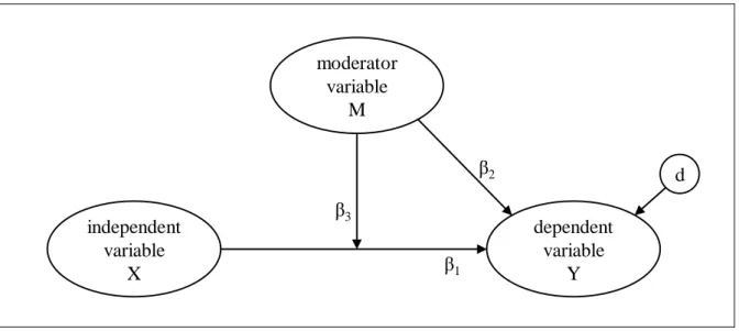
relationship within the structural model. This means that one construct moderates the direct relationship between two other constructs. As an exemplary model we will use a basic structural model consisting of a dependent variable Y, an independent variable X, and a moderator variable M. As shown in Figure 1, the moderating effect (β3) is symbolized by an arrow pointing to the relationship between X and Y (i.e., β1) that is hypothesized to be moderated. independent variable X dependent variable Y moderator variable M d β1 β3 β2
Figure 1: A basic model with a moderating effect (β3)
However, such a structural model cannot be drawn in the available software for variance-based SEM such as ADANCO or SmartPLS. In order to estimate moderating effect, a more profound look at PLS path modeling is required. PLS path models are traditionally estimated in two steps: (1) An iterative algorithm provides approximations for each latent variable (so-called latent variable scores) and (2) linear regression is applied to these scores. Because of this procedure, most of the recommendations for analyzing moderating effects in multiple regression hold for PLS path modeling as well. Thus the two basic approaches as discussed in the literature on the estimation of moderating effects in multiple regression (see for example Aiken and West, 1991, Spiller et al., 2013), namely the integration of an interaction term and the use of group comparisons, can be applied (with adaptations) in PLS path modeling.
The interaction term approach is a straightforward implementation of a moderating effect if the moderator variable influences the strength of the moderated relationship in a linear fashion (as shown in equation (4)). As long as the moderator variable is dichotomous, the interaction term approach and the group comparison approach (see Sarstedt et al., 2011, for a tutorial on PLS multigroup analysis) lead to quite comparable results. However, the group comparison approach is suboptimal for continuous moderating variables because due to the necessary dichotomization a part of the moderator variable’s variance is lost for analysis. Only if the moderator variable is categorical (for instance in experimental designs, see Streukens et al., forthcoming), or if the researcher wants a quick overview of a possible moderator effect, should the group comparison approach be considered (Henseler and Fassott, 2010, p. 721). Therefore, this tutorial discusses issues related to the integration of an
interaction term as an additional latent variable in the PLS path model only.
In order to develop the moderation model, we first depart from the main effects model, which simply contains the linear effects of X and M on Y. This leads to Equation (1):
Y = β0’ + β1’ ∙ X + β2’ ∙ M + d’ (1) Here, β0’ is the intercept, and β1’ and β2’ are the slopes of X and M, respectively, while the unexplained variance is captured by the error term d’. Obviously, β1’ and β2’ are first partial derivatives quantifying the change in Y depending on the change in one predictor if the other predictor is held constant.
In moderated multiple regression, the idea of a moderating effect is that the slope of the independent variable is no longer constant, but depends linearly on the level of the moderator. The structural equation of the model depicted in Figure 1 can thus be formulated as follows:
Y = β0 + (β1 + β3 ∙ M) ∙ X + β2 ∙ M + d (2) Equation (2) can be mathematically rearranged to have either of the following two forms:
Y = β0 + β1 ∙ X + β2 ∙ M + β3 ∙ (X ∙ M)+ d (3)
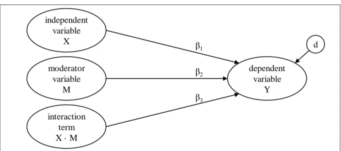
In Equation (3), the so-called interaction term (X ∙ M) is introduced, built by multiplying the independent and the moderator variable. This answers the question of how moderating effects can be integrated into a PLS path model. The interaction term can be treated as an additional construct leading to the graphical representation of Equation (3) as shown in Figure 2. Equation (4) provides another way of looking at the model: For a fixed level of M, (β0 + β2 ∙ M) is the intercept, and (β1 + β3 ∙ M) is the slope of the independent variable X. In particular, β0 and β1 represent the intercept and the slope of X when M equals zero.
moderator variable M dependent variable Y independent variable X β d 1 β3 β2 interaction term X · M
Figure 2: Transcript of the model in Figure 1 for PLS path models
Typically, the regression coefficients obtained from Equation 1 will differ from those of Equations 2 to 4. This fact is emphasized by the use of the apostrophe for the regression coefficients in Equation 1. As soon as the interaction term is integrated into the regression function, the regression parameters no longer represent main effects but single effects (sometimes also called “simple effects”). Single effects mean that they describe the strength of an effect when all the other components of the interaction term have a value of zero. Thus if the value of the moderator variable M is zero, then the dependent variable Y is expressed by the independent variable X in the form of a single regression with the intercept β0 and the slope β1. How the intercept and the slope of this single regression change when the moderator variable has a value different from zero can be seen from equation (4). It should be noted that “the interaction term, i.e. the product of the independent variable X and the moderator
variable M, is as such commutative. This fact implies that mathematically it does not matter which variable is the independent and which one the moderator variable. Both the
interpretations are equally legitimate” (Henseler and Fassott 2010, p. 719).
As Henseler and Chin (2010) point out PLS does not calculate the regression parameters as used in equation (3). The reason for this is that PLS estimates a regression in which all variables, including the interaction term, are standardized. Thus the regression equation of the structural model as estimated by PLS takes the following form:
Ystd = b1 ∙ Xstd + b2 ∙ Mstd + b3 ∙ (Xstd ∙ Mstd)std + e (5) Equation (5) takes into account that the product of two standardized variables is not necessarily a new standardized variable. Rather the product has to be standardized before entering the regression. As a consequence, the value of b1 for a particular score of M cannot be derived by simply rearranging equation (5). However, standardized regression coefficients can be transformed into unstandardized regression coefficients taking into account the
standard deviations of the dependent and independent variables. Equation (6) shows this relationship for the independent Variable X.
β1 = (sY / sX) ∙ b1 (6)
We can use this relationship to derive the size of b1 for a specific score of M by replacing the left side of equation (6) with the unstandardized regression coefficient (β1 + β3∙M) from equation (4). Replacing β1 (and β3) with the right side of equation (6) and multiplying with (sX / sXY) leads to equation (7) providing b1(M) as a function of M and the regression coefficients b1 and b3 as calculated from equation (5), i.e. representing M equal zero.
b1 (M) = b1 + (sX/sXM)∙ b3∙M (7) While PLS computes standardized regression coefficients according to equation (5), some variance-based SEM software like ADANCO (Henseler and Dijkstra, 2015) provides the unstandardized scores of the latent variables. Thus the parameters in equation (3) can easily
be calculated by regressing the scores of Y to the scores of X, M, and X ∙ M. In addition, the standard deviations needed for equation (7) can be calculated.
Modeling Moderating Effects via Interaction Terms
While the use of the interaction term X ∙ M as additional latent variable in the PLS path model covering the product of the exogenous and the moderator variable looks
straightforward, there are several approaches available to provide indicators for this
interaction term. The product indicator approach and the two-stage approach are often used when modeling moderating effects in PLS path models. Henseler and Chin (2010) elaborated two more approaches (the orthogonalizing and the hybrid approach) and compared them with the former two approaches in a Monte Carlo experiment. They concluded that the
orthogonalizing approach is recommendable under most circumstances whereas the hybrid approach does not outperform the other approaches and in addition is not readily available in PLS software packages. Thus we will not deal with the hybrid approach in this paper.
Product Indicator Approach
The basic idea of the product indicator approach is to build product terms between the indicators of the latent independent variable and the indicators of the latent moderator variable (Kenny and Judd, 1984). These product terms serve as indicators of the interaction term in the path model. Chin et al. (1996, 2003) were the first to apply this approach to PLS path
modeling. They suggested to calculate the products of each indicator of the latent independent variable with each indicator of the moderator variable. Thus all possible pairwise products become the indicators of the latent interaction variable (see Henseler and Chin, 2010, for a discussion why all possible products should be used).
However, the product indicator approach is restricted to common factors (see Fassott and Henseler, 2015, for a discussion of the differences between factor and composite
underlying factor, the resulting product indicators will not necessarily tap into the same underlying interaction effect (Chin et al. 2003, appendix D). Nevertheless, if the independent and the moderator variable are both single-indicator variables, the product term can be built, because in PLS path modeling latent variables with only one indicator are set equal to this indicator. Thus, if both the independent and the moderator variable have only one indicator, the product indicator approach is identical with stage 2 of the two-stage approach described in the next section. In any case, researchers should pay attention to the reliability of the
interaction term. Since the error terms of the product indicators cannot be expected to be fully orthogonal, it is better not to let PLS estimate the reliability of the interaction term, but to manually define it as the product of the reliability of the independent and the reliability of the moderator variable.
Two-Stage Approach
If the independent and/or the moderator variable use composite measurement models, the pairwise multiplication of indicators is not advisable. Instead, one can exploit that PLS path modeling explicitly approximates construct scores. In this way, the interaction term does not need product indicators at all. Henseler and Fassott (2010) suggest the following two-stage approach:
Stage 1: In the first stage, the main effects PLS path model is run in order to obtain
construct scores of the independent and the moderator variable. These scores are calculated and saved for further analysis.
Stage 2: In the second stage, the interaction term X ∙ M is built up as the element-wise
product of the construct scores of X and M. This interaction term as well as the latent variable scores of X and M are used as independent variables in a
multiple regression on the latent variable scores of Y.
This approach is also applicable if the independent or the moderator variable is modeled as common factor. In this case, the correlations of the interaction term with the other
constructs in the model need to be disattenuated by the product of the reliabilities of the independent and the moderator variable.
Orthogonalizing Approach
Both the product indicator and the two-stage approach will provide an interaction term which can be correlated to both the independent and the moderator variable. As a
consequence, the typical phenomena of multicollinearity may occur, such as unexpected signs of coefficients or increased standard errors. Although multicollinearity caused by interaction terms is not a problem per se, it can hamper the interpretation (Echambadi & Hess, 2007). This negative consequence can be avoided by adapting the use of residual centering as described by Lance (1988) for moderated multiple regressions. Little et al. (2006) suggested an orthogonalizing approach for modeling interactions among latent variables which was applied to PLS path modeling by Henseler and Chin (2010). It is essentially a two-step OLS procedure where a product term is regressed on its factors and the residuals of the regressions are then used as indicators of the latent interaction variable.
As a consequence of the orthogonality of the interaction term, the parameter estimates of the effects of X and M in the PLS path model are identical to the parameter estimates of the direct effects in a model without interaction term, i.e. they represent main effects of the exogenous and the moderator variable respectively according to equation (1). However, the standardized regression coefficients may be slightly different (see Table 3).
While Henseler and Chin (2010) have demonstrated the superiority of the
orthogonalization approach for common factor measurement models in terms of parameter and prediction accuracy, it remains unclear whether the orthogonalization approach
outperforms the two-stage-approach when composite models are used. Furthermore, the orthogonalization approach has the disadvantage of lower statistical power. If an interaction effect is found to be nonsignificant by the orthogonalizing approach, the reason could be that this approach did not have enough statistical power to find it. In such a case Henseler and
Chin (2010) propose using additionally the more powerful two-stage approach to test whether an interaction effect is significant or not. Furthermore, if the researcher is interested how the impact of the independent variable X changes for different scores of the moderator variable M (i.e. examining single effects), the orthogonalizing approach is not suitable.
Scaling of the Variables
The indicators used for building the interaction term must have metric scales. In the case of a dichotomous indicator it is possible to dummy code (0 = category 1, 1 = category 2) or contrast code (-1 = category 1, 1 = category 2) this indicator and use it as a metric variable. As the single effect of the exogenous variable describes the effect when the moderator variable equals zero, a dummy coded moderator variable allows a straightforward interpretation of this single effect. Therefore, dummy coding should be used for a dichotomous (single) indicator variable instead of contrast coding.
In case of a latent moderator variable M with multiple indicators again the single effect of the exogenous variable X describes the slope of the regression of X on Y when M has a value of zero. In PLS path models, the latent variable scores are calculated as linear combinations of the corresponding indicators. Thus the linear combination of the corresponding indicators must provide a value of zero. This is generally possible using the original scale of the indicators if each indicator has the value of zero in its scale. Otherwise M (as linear
combination of the indicators in their original scales) could (theoretically) only have a value of zero if there are opposite signs (i.e., negative and positive values) in some of the indicator scales or opposite signs in the weights PLS uses to calculate the latent variable scores. This will often not be the case, i.e., in many cases zero will not be an existing value on the scale of M providing a single effect which is not meaningful.
More meaningful single effects can be obtained by means of centering. Adding or subtracting a constant from the original variable to recode it makes the value of this constant the zero point of the recoded scale (Spiller et al., 2013). A straightforward way to select the
value of the constant is to subtract the mean, i.e., center the latent variable scores (Aiken and West 1991). Centering a latent variable can easily be accomplished by centering all its indicators. This is strongly recommendable for the product indicator approach. When using the two-stage approach, the original indicators can be used though in step 1 and then the unstandardized construct scores can be centered before entering step two. When both the exogenous and the moderator variable are centered, then the single effect of the exogenous variable describes the slope of the regression of X and Y when M has a value of its mean. In addition to this interpretation advantage, centering X and M may considerably lessen
multicollinearity in the structural model introduced by the interaction term (Aiken and West, 1991, p. 35).
To calculate the change in the intercept and/or the slope of the independent variable X according to Equation (4), it is necessary to use the indicators of the moderator variable in their original scale. The independent variable should still be centered to lower the
multicollinearity introduced to the structural model by the interaction term as a product of two other model variables. This has no effect on the regression coefficients of the independent variable. However, if a researcher is interested in the change of the intercept as well, than the independent variable X must be in its original scale as well.
Whilst centering is advantageous for metric exogenous and/or moderator variables, it is not necessary for the dependent latent variable Y. As Aiken and West (1991, p. 35) point out: “Changing the scaling of the criterion by additive constants has no effect on regression coefficients in equations containing interactions. By leaving the criterion in its original (usually uncentered form), predicted scores conveniently are in the original scale of the criterion. There is typically no reason to center the criterion Y when centering predictors”. If only the relative impact of the predictors is of interest, researchers may use standardized indicators for X and M. Then also the indicators of the dependent variable Y should be standardized (Henseler and Fassott, 2010).
Example Application
In order to demonstrate the different approaches, we used a data set (n= 196) from a study on the impact of CRM (customer relationship management) tools on relationship quality and loyalty in e-tailing (Fassott, 2004). In this study a moderating effect of online deal proneness on the effect of relationship investment on relationship quality was tested by a multi-group analysis in covariance-based SEM. Relationship investment mediated the impact of CRM tools, which an online shop can apply, on the relationship quality. One dimension of
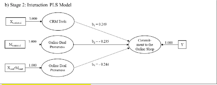
relationship quality, namely commitment to the online-shop, showed a considerable influence of online deal proneness on the effect of relationship investment. As shown in Figure 3 we test the moderating effect of online deal proneness (=M) on the relationship between CRM tools (=X) and commitment (=Y).
Figure 3: Results of basic PLS path models
We estimated the different models using ADANCO (Henseler and Dijkstra 2015). The main effect model was estimated with all the indicators in their original scale, which was a 7-point rating scale from one to seven. Some key data of the resulting constructs are shown in Tables 1 and 2. For all three variables there is a minimum score of one and a maximum score of seven. The unstandardized construct scores (as well as the standardized construct scores) were stored for the two-stage approaches. In addition, we centered the unstandardized
construct scores of the independent and the moderator variable by subtracting their respective means. The unstandardized construct scores of X and M were multiplied and this interaction term was regressed on the unstandardized X- and M-scores. The resulting error term of the regression was saved as indicator for the interaction term in the orthogonalizing approach. Finally, the product of the centered (as well as the standardized) X- and M-scores was saved.
While on average the commitment to the online shop is quite high, the respondents show rather low online deal proneness. On average the resulting CRM variable score is close to the middle of the scale. For all three variables the lowest variable score is one and highest is seven.
Mean Standard Deviation
Y 5.064 1.841
M 2.618 1.612
X 4.354 1.490
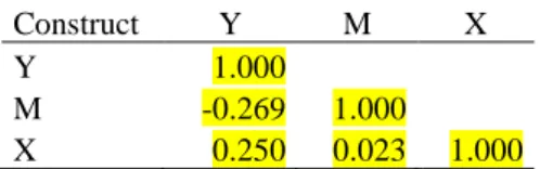
The commitment variable shows a moderate negative correlation to the moderator and a moderate positive correlation to the independent variable. The moderator is very weakly correlated to the independent variable (see Table 2).
Construct Y M X
Y 1.000
M -0.269 1.000 X 0.250 0.023 1.000
Table 2: Construct Correlations
Table 3 provides the results of the different models. For every model we report the PLS results computed by ADANCO in the first row. In the second row we show the
unstandardized path coefficients in addition, which were calculated by OLS-regressions in MS Excel using unstandardized construct scores. The significance of the estimated PLS-parameters was assessed based on bootstrapping. The strength of the moderating effect was assessed by comparing the proportion of variance explained (as expressed by the
determination coefficient R²) of the main effect with the R² of the full model. Thus drawing on Cohen (1988, p. 410-414) we calculated the effect size f² with the formula shown in Equation (8). The f²-scores of every (independent) variable are part of the standard output of ADANCO.
𝑓X∙M2 =𝑅model with interaction term2 −𝑅model without interaction term2
Estimation Method
Unstandardized Estimates Standardized Estimates R²adj Effect Size β0 β1 β2 β3 b1 b2 b3 f²X f²M f²X·M Recommendable approaches
Main effects only
4.523 0.314 −0.316 ― 0.256 −0.275 ― 0.129 0.076 0.088 ― Orthogonalizing 4.523 0.314 −0.316 −0.179 0.254 −0.277 −0.240 0.184 0.080 0.095 0.072 Two-stage (X and M centered)
5.073 0.308 −0.268 −0.179 0.249 −0.235 −0.244 0.184 0.077 0.066 0.072
Approaches neglecting the scaling recommendations
Two-stage (X, M and Y standardized)
0.005 0.251 −0.232 −0.234 0.251 −0.232 −0.245 0.183 0.078 0.065 0.072 Two-stage (X, M and Y standardized;
X·M based on unstandardized X and M) 1.144 0.640 0.469 −0.100 0.640 0.469 −0.880 0.186 0.148 0.027 0.075 Two-stage
2.389 0.778 0.513 −0.179 0.629 0.450 −0.858 0.184 0.143 0.025 0.072 Table 3: Results of the different approaches
Moderating effects f²X∙M of at least 0.02 may be regarded as weak, effect sizes from 0.15 on as moderate and effect sizes of 0.35 and higher as strong (Cohen, 1988). All the path coefficients shown in Table 3 are significant. There is a weak negative moderating effect of the moderator variable, i.e. the effect of CRM tools on commitment gets lower when the online deal proneness of the respondents gets higher. The interaction effect (unstandardized coefficient and effect size f²X∙M) is identical for the orthogonalizing and the two two-stage approaches, which differ on the use of centered vs. the original unstandardized construct scores. The latter may not always be the case. In our case the correlations between the constructs are quite low, thus the two-stage model using the unstandardized construct scores is not affected by multicollinearity issues. If multicollinearity is high and the original
unstandardized construct scores are used, then curious results may arise like inflated standard deviations from bootstrapping or correlation sizes greater than one.
Concerning the (unstandardized) path coefficient β1 of the independent variable we see that the single effect lowers considerably (0.778 vs. 0.314) if the score of the moderating variable rises from zero to its mean (2.618). However, it should be noted, that a score of zero is outside our measurement model. The orthogonalizing approach provides the main effects for X and M, i.e. the unstandardized coefficients are identical to the main effects model without the interaction term.
So far, we have tested that there is a significant weak moderating effect. The basic principle of a moderator effect is its influence on the size of the effect the independent variable X has on the dependent variable Y. From Table 3 we can see, how strong the effect of X on Y is, when the moderator variable M has a score of its mean (and a M-score of zero outside our measurement model). How does this effect size change for other values of M? The answer is provided by a spotlight analysis (Spiller et al. 2013). This can easily be
accomplished in the two-stage approach by modifying the scores of M and (via the
equals one, we have to subtract one from the original unstandardized construct score. This can be done for every value of M. In fact, the two-stage model (X and M centered) in Table 3 did the same by subtracting the mean (here 2.618) from the original construct score. Thus, we could add these results in Table 4 between the rows of M=2 and M=3.
The results of the spotlight analysis are shown in Table 4. For M equals zero we use the unstandardized M-score of the main effects model. Although this score is outside of our measurement model we need the regression coefficients in order to simply compute regression coefficients for other values of M. While Table 4 shows the results of PLS computations, one can easily generate the unstandardized coefficients as well as the
standardized coefficients using the equations (4) and (7) respectively, with the results for M=0 and changing the value of M.
M Intercept β0 Slope β1 Slope b1 Comment
0 5.774 0.778 0.629 Value of M = 0 was not measured
1 5.506 0.599 0.484
2 5.238 0.419 0.339
3 4.970 0.239 0.194
4 4.703 0.060 0.048 insignificant slope (two-sided, α=0.05) 5 4.435 -0.120 -0.097 insignificant slope (two-sided, α=0.05) 6 4.167 -0.299 -0.242 insignificant slope (two-sided, α=0.05)
7 3.899 -0.478 -0.387
Table 4: Spotlight analysis using two-stage PLS with centered X-scores
In our example, we see that the effect of X on Y is non-significant for M equal four, five, or six. For M=7 the direction of the effect of CRM tools on commitment gets significantly negative. Thus the managerial implications of these results point in two different directions. (1) If the customers of an online shop show low online deal proneness the online shop can raise their commitment (and considering the positive impact of commitment to loyalty finally their loyalty) to the online shop by improving its CRM tools. (2) If the customers of an online shop show very high online deal proneness the improvement of CRM tools would be
example demonstrates the value of a spotlight analysis, i.e. the analysis of moderating effects should be more than just testing for the significance of the regression coefficient of the interaction term and its effect size.
Considering the simplicity of computing the path coefficients based on the results for M=0, it is still necessary to run PLS models in the spotlight analysis. First, PLS models for different values of M need to be run to determine the significance of the intercept and the path coefficients of X and to compute the effect size f²X. As different values of M will be used, the positive impact of centering M on multicollinearity diminishes. Thus problems with invalid results due to multicollinearity may be detected by comparing the PLS results with the results using the equations in Table 4. Second, this equations are based on the PLS results for M equal zero. It may happen, that for this M-score multicollinearity issues may lead to invalid results. This can be detected if the unstandardized coefficient of the interaction term differs between the two-stage approach and the orthogonalization approach. In this case it is still possible to compute valid results for the simple effects, if we have valid results for the centered M (again compare the path coefficients of the interaction term obtained from the two-stage and the orthogonalizing approach).
Concluding Recommendations
Having discussed different approaches to analyze moderation effects including at least one composite variable with PLS we recommend the following procedure. Note, that this is also a possible procedure if all variables are common factors.
1. Run the main effects PLS model using the indicators in their original scale. Save the unstandardized construct scores for further analysis. In addition center the construct scores of the independent (X) and the moderator (M) variable. Compute both the product of the original unstandardized construct scores of X an M as well as the product of their
centered versions. Finally, compute the error term needed as indicator of the interaction term in the orthogonalizing approach by regressing the product of the original unstandardized construct scores of X an M on the original unstandardized construct scores of X an M.
2. Run the orthogonalizing approach to determine the significance of the interaction term’s path coefficient and effect size f²X·M. If this is the only aim of the analysis, then stop here.
3. In case the coefficient obtained from the orthogonalizing approach is not significant, check with the two-stage approach whether this may be just due to the lower power of the orthogonalizing approach. In this case or if the two-stage approach is necessary because the single effects are of interest compute also the unstandardized coefficient β3 by running an OLS-regression using the unstandardized construct scores resulting from the orthogonalizing model.
4. Prepare the data sheet for stage two of the two-stage approach. Especially, add centered scores of the construct scores for the independent variable X and the moderator variable M. If a spotlight analysis is planned, then additional variables subtracting constants other than the mean of M may be calculated in addition to the original unstandardized construct score of M. Compute interaction terms by multiplying each of these different M variables with the centered X-variable.
5. Run at least two PLS models for the unstandardized construct score of M (M=0) and for centered M-score. Use the (calculated) construct scores as single indicators for the variables (X centered, Y as unstandardized construct score, the respective product of the centered X with the M in use). Compute the unstandardized regression coefficients by running OLS-regressions using the unstandardized construct scores resulting from the PLS runs. Cross-check the unstandardized coefficient of the interaction term with the coefficient of the orthogonalizing approach.
6. If a spotlight analysis is intended, run the model for other values of M as well. Cross-check the PLS results with the coefficients computed based on the coefficients of the PLS run for M=0.
Using this procedure will require several computations outside current PLS software. If a PLS software provides results, especially the unstandardized construct scores, in the format of tabulation programs like MS Excel this will be quite easy. However, as our procedure uses the unstandardized regression coefficients in addition to the standardized coefficients provided by PLS, PLS software packages could support moderation analysis by providing these
References
Aiken, L. S. and West, S. G. (1991). Multiple regression: testing and interpreting
interactions. Newbury Park: Sage.
Baron, R. M. and Kenny, D. A. (1986), “The moderator-mediator variable distinction in social psychological research: conceptual, strategic, and statistical considerations”, Journal of
Personality and Social Psychology, Vol. 51 No. 1, pp. 1173-1182.
Chin, W. W., Marcolin, B. L., and Newsted, P. N. (2003), “A partial least squares latent variable modeling approach for measuring interaction effects: Results from a Monte Carlo simulation study and an electronic-mail emotion/adoption study”, Information Systems
Research, Vol. 14 No. 2, pp. 189-217.
Chin, W.W., Marcolin, B. L., and Newsted, P. R. (1996), “A partial least squares latent variable modeling approach for measuring interaction effects. Results from a Monte Carlo simulation study and voice mail emotion/adoption study”, in J. I. DeGross, S. Jarvenpaa, & A. Srinivasan (Eds.), Proceedings of the Seventeenth International Conference on Information
Systems, Cleveland, OH, pp. 21-41.
Cohen, J. (1988). Statistical Power Analysis for the Behavioral Sciences. Hillsdale, NJ: Lawrence Erlbaum.
Dijkstra, T.K. and Henseler, J. (2015), “Consistent partial least squares path modeling”, MIS
Quarterly, Vol. 39 No. 2, pp. 297-316.
Dijkstra, T.K. and Schermelleh-Engel, K. (2014), “Consistent partial least squares for nonlinear structural equation models”, Psychometrika, Vol. 79 No. 4, pp. 585-604. Echambadi, R. and Hess, J. D. (2007), “Mean-centering does not alleviate collinearity problems in moderated multiple regression models”, Marketing Science, Vol. 26 No. 3, pp. 438-445.
Fassott, G. (2004), “CRM tools and their impact on relationship quality and loyalty in e-tailing”, International Journal of Internet Marketing and Advertising, Vol. 1 No. 4, pp. 331-349.
Fassott, G. and Henseler, J. (2015), “Formative (measurement)”, in: Cooper, C., Lee, N. and Farrell, A. (Eds.). Wiley Encyclopedia of Management, Volume 9, Marketing, 3rd ed.
Chichester: Wiley, pp. 1-4.
Henseler, J. and Chin, W.W. (2010), “A comparison of approaches for the analysis of interaction effects between latent variables using partial least squares path modeling”,
Structural Equation Modeling, Vol. 17 No. 1, pp. 82-109.
Henseler, J. and Dijkstra, T.K. (2015). ADANCO 1.1. Kleve, Germany: Composite Modeling. Henseler, J. and Fassott, G. (2010), “Testing moderating effects in PLS path models: an illustration of available procedures”, in Vinzi, V.E. et al. (Eds.), Handbook of Partial Least
Henseler, J., Hubona, G., and Ray, P. (2016), “Using PLS path modeling in new technology research: Updated guidelines”, Industrial Management & Data Systems, Vol. 116 No. 1, pp. 2-20.
Jaccard, J., and Turrisi, R. (2003). Interaction effects in multiple regression, 2nd ed. Thousand Oaks: Sage.
Kenny, D. A., and Judd, C. M. (1984), “Estimating the nonlinear and interactive effects of latent variables”, Psychological Bulletin, Vol. 96 No. 1, pp. 201-210.
Lance, C. E. (1988), “Residual centering, exploratory and confirmatory moderator analysis, and decomposition of effects in path models containing interactions”, Applied Psychological
Measurement, Vol. 12 No. 2, pp. 163-175.
Little, T. D., Bovaird, J. A., and Widaman, K. F. (2006), “On the merits of orthogonalizing powered and product terms: Implications for modeling interactions among latent variables”,
Structural Equation Modeling, Vol. 13 No. 4, pp. 497-519.
Nitzl, C., Roldán, J. L., & Cepeda Carrión, G. (2016), “Mediation analysis in partial least squares path modeling: helping researchers discuss more sophisticated models”, Industrial
Management & Data Systems, in print.
Sarstedt, M., Henseler, J., and Ringle, C. M. (2011), “Multi-group analysis in partial least squares (PLS) path modeling: alternative methods and empirical results”, Advances in
International Marketing, Vol. 22, pp. 195-218.
Spiller, S.A., Fitzsimons, G.J., Lynch, J.G., Jr., and McClelland, G.H. (2013), “Spotlights, floodlights, and the magic number zero: simple effects tests in moderated regression”, Journal
of Marketing Research, Vol. 50 April, pp. 277-288.
Streukens, S. and Leroi-Werelds, S. (2016), “PLS FAC-SEM: An illustrated step-by-step guideline to obtain a unique insight in factorial data”, Industrial Management & Data