Market microstructure model: study of varations of exchange rate for Asia and Latin America.

(1)

C I G E

CENTRO DE INVESTIGAÇÃO EM GESTÃO E ECONOMIA

UNIVERSIDADE PORTUCALENSE – INFANTE D. HENRIQUE

DOCUMENTOS DE TRABALHO

WORKING PAPERS

n. 2 | 2008

M

A

R

K

E

T

M

I

C

R

O

S

T

R

U

C

T

U

R

E

M

O

D

E

L

:

S

T

U

D

Y

O

F

V

A

R

I

A

T

I

O

N

S

O

F

E

X

C

H

A

N

G

E

R

A

T

E

F

O

R

A

S

I

A

N

D

L

A

T

I

N

A

M

E

R

I

C

A

Vasco Salazar Soares, ISVOUGA, Professor of the Finance Department vsalazarsoares@gmail.com

Antonieta Lima, ISVOUGA, Assistant of the Finance Department antonietasousalima@gmail.com

(2)

M

MAARRKKEETTMMIICCRROOSSTTRRUUCCTTUURREEMMOODDEELL::

S

STTUUDDYYOOFFVVAARRIIAATTIIOONNSSOOFFEEXXCCHHAANNGGEERRAATTEEFFOORRAASSIIAAAANNDDLLAATTIINNAAMMEERRIICCAA

Vasco Salazar Soares, ISVOUGA, Professor of the Finance Department vsalazarsoares@gmail.com

Antonieta Lima, ISVOUGA, Assistant of the Finance Department antonietasousalima@gmail.com

Abstract

The paper studies the commercial relations between Europe and its principal commercial partners, such as Asia and Latin America, for the period of 1999 to 2007. The methodology appeals to the correlation analysis of the variables of the model and the autocorrelation of the exchange rate variation variable, to the Augmented Dickey-Fuller (1979) and Philips-Perron tests (1988), and finally, to the market microstructure model suggested by Medeiros (2005).

Medeiros (2005) model, when applied to the Asian and Latin American markets, in their relations with Europe, give us more consistent and stronger results, although R2 is still very low. An estimation with ARCH/GARCH-M methodology increases the model capacity substantially, confirming the previous results of Medeiros (2005).

(3)

I - INTRODUCTION

The purchasing power parity theory had its origin in the mercantilist literature of the XVII century, having itself become prominent with Gustav Cassel [1, 2] in the beginning of the XX century. The purchasing power parity is known as an essential condition of the exchange rate balance, in the long run, in a dynamic model of the exchange rate determination.

This theory establishes that the exchange rate between currencies is in balance, when the purchasing power is the same in different countries. This means that, the exchange rate will have to equal the price level between different countries, considering one or some fixed goods and services, when expressed in the same currency. When the country internal price level increases relatively to other countries (when a country has inflation), the exchange rate of this country has to depreciate to return to the purchasing power parity level. Usually, to calculate the purchasing power parity between two countries, we compare the price of an identical standard product between different countries. However, one of the main problems inhabits this comparison. In fact consumers, in different countries, consume several products and services sufficiently different (internationally non-traded goods), making this purchasing power parity comparison very difficult.

Given the controversy and lack of precision of the purchasing power parity theory, and seeing that this one only presents the exchange rate variation inflation differences between countries, some authors have considered alternative models. Some of them are Evans and Lyons (2002) [3] who introduced a new proposal. Amplifying the traditional macroeconomics analysis, they inserted a variable from market microstructure finance.

According to O'Hara (1995) [4], market microstructure is defined as the “processes and the outcomes of exchanging assets under explicit negotiation rules” (order flow). By doing this, Evans and Lyons (2002) [3] created a new class of models, based on microstructure finance, which include variables that the macroeconomic models omit.

The model can be expressed in the following form,

[1] ∆Pt = ∆mt + λ ∆xt

where,

∆P, is the exchange rate change;

∆m, are innovations concerning macroeconomic information (e.g., interest rate changes); λ, is a positive constant;

(4)

t, refers to time;

x, is the accumulated order flow.

With intention to reach the stated goals, Medeiros (2005) [5] considered two alterations to the equation above presented. Firstly, the public information increment (∆m) is defined as the change in the interest rate differential (foreign minus internal domestic rate), i.e. ∆m = ∆(i* - i), plus a white-noise random term, where i* is the nominal interest rate associated to the foreign currency and i is the nominal interest rate associated to the local currency. However, ∆m could also be a function of other macroeconomic fundamentals. The interest rate differential was privileged seeing that is the main predictor of exchange rate variations in macroeconomic models, and also because it is a variable with available daily data. Secondly, the dependent variable ∆P is replaced by the change in the log of the spot exchange rate, ∆p. With this replacement, the specification takes the form,

[2] ∆pt = α∆(i*t – it) + β∆xt + εt

where,

∆pt, is the change in the log of the spot exchange rate (number of real for USD, being USD the currency quoted in the original model);

∆(i*t – it), is the change in the interest rate differential (i*t is the interest rate of Real and, it is the interest rate of USD, in the original model);

∆xt, is the order flow;

α and β are regression parameters; εt ~ N(0, σ2), is the error term.

To the coefficient α is expected a positive signal, based on the sticky-price monetary model, since an increase in the foreign interest rate i* requires an immediate appreciation of the foreign currency. The coefficient β is also expected to have a positive signal, indicating that reserves stock of the quotation currency increases with the valuation of the quoted currency.

An important aspect to be pointed out is that, in general, the theoretical models, including Evans and Lyons’s (2002) [3], consider that investors are risk neutral, so that risk premia are rarely included in these models. However, the poor performance of some exchange-rate models could be attributed to the omission of relevant variables such as risk factors, as referred by Macdonald and Taylor (1992) [5]. If investors are risk averse, it is necessary to take into account the premium that compensates investors for the risk of holding assets in foreign currency (e.g. Brazilian currency: real).

(5)

5

Given capital mobility, the interest rates of the quotation currency (e.g. Brazilian currency: real) must be equal to the interest rate of the quoted currency (e.g. USD) plus two-risk premia. The first risk premium compensates the investor for the depreciation of the quotation currency (e.g. Brazilian currency: real), and it is measured by the future quoted currency (e.g. USD). The second risk compensates the investor for the risk of government debt moratorium, capital controls, and other movements that may affect the return in USD of the investment. The first risk premium is denominated exchange-rate risk; the second, country risk.

Thayer Watkins (2005) [7] defines country risk premium as an increment in interest rates that would have to be paid for loans and investment projects in a particular country, compared to some standard measured. One way to calculate country risk premium for a certain country is to compare the interest rate that market establishes for a standard measure (e.g. central government debt), and compare it to the same measure with an benchmark country, for example the USA. To be comparable both measures must have the same maturity and be paid in the same currency, say USD. This measures uniformity is very important; otherwise interest rates differential would reflect inflation rate differential in the two countries, instead of only reflecting non-payment risk. To notice that relevant interest rate is the market-determined yield to maturity rather than the coupon interest rate. The coupon interest rate is only important if issuers set coupon rate equal to the yield to maturity. In mathematical notation,

[3] ρ = [(1 + a) / (1 + b)] – 1

where,

ρ, is the country risk premium;

a, is the country interest rate to which country risk premium is being calculated;

b, it refers to country interest rate in relation to which we are establishing the comparison. For example, if borrows are USD denominated, the standard measure could be the USA.

In the same way, Eugene Famma (1984) [8] derived and tested a model for the joint measurement: risk premium and future exchange rates. In this direction, he used the nine most internationally negotiated currencies in the period between 1973 and 1982, and found evidence that both variables float over the time. This author concluded that, on the one hand, the risk premium and the expected depreciation rate for the forward market has a negative correlation. On the other hand, he concluded that most of the future exchange rate variation is due to risk premium variation.

With all this, Medeiros (2005) [5] amplified Evans and Lyons’s (2002) [3] model, incorporating a variable associated with country risk, the risk premium. This hypothesis constitutes one possible explanation to exchange rate volatility in the long term. The model was defined in the following form,

(6)

[4] ∆pt = ∆(i*t – it) + ∆xt + ∆rt + εt

where,

∆rt, is the daily change in the country risk premium. It was assumed that since country risk is associated to the market’s perception regarding the country’s political and economic situation, it is an exogenous variable.

With the proposal of a risk premium existence in the financial markets, this paper intends to give a new contribute in exchange rate variations study, specifically, by studying cambial variations between euro and Asian and Latin America country currencies.

Therefore, following Medeiros’s (2005) [5] market microstructure model, we collected, to the mentioned markets, monthly samples: spot exchange rate, reserves, internal interest rate, external interest rate, and consumer price index.

To represent commercial relations between Europe and the Asian market, we chose China, India, South Korea, Indonesia and Thailand for the period from 1999 to 2007. To represent Europe and Latin America relations we chose Brazil, Argentina, Venezuela, and Colombia, for the decurrently period from 1999 to 2007.

(7)

I

III––MMEETTHHOODDOOLLOOGGYYAANNDDSSAAMMPPLLEE

In a global world, where the economies interact more and more, the exchange rate assumes an important role in the study of international finances, for example, in the competitiveness of each country, in import and export operations, in the generation of work, in the expansion of domestic market, in the control of inflation, in the financial flows, and in the economic growth.

In this sense, to have a real perception of the exchange rate variation impact in commercial relation between countries constitutes, indeed, an important factor for all the economic agents that works with the market of goods and services, and with the monetary market.

This article studies the commercial relations between Europe and some of its commercial partners, Asian and Latin America markets, for the period since 1999 to 2007.

The methodology initially appeals to the Pearson correlations analyses to the model variables, following the autocorrelations analyses with Akaike Information Criterion (1974) [10], being indicated in this work the autocorrelations for the most significant economies, India and China.

The methodology appeals to Augmented Dickey-Fuller (1979) [9, 15] and Philips-Perron (1988) [11] tests, and to the market microstructure model.

I

III..11..SSaammpplleeaannddddaattaa

This empirical study is based on a monthly economic series, available in central banks of each country and in European Central bank, concerning market microstructure model variables: exchange rate, total reserves, intern and extern interest rate one month1_{, and consumer price index. To express country}

risk premium variations, we calculated this index according with Thayer Watkins (2005)2_[7].

As we have already said, this article intention is to try to explain the main factors responsible for exchange rate variation between euro and Asian and Latin America currencies.

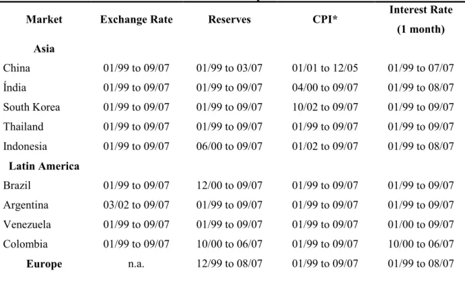
Data samples are expressed in Table 1 ("Sample Periods"). All modulation was carried through with software Eviews 3.0.

1 It was the only rate common to all the countries.

(8)

Table 1: Sample Periods

Market Exchange Rate Reserves CPI* Interest Rate (1 month) Asia China 01/99 to 09/07 01/99 to 03/07 01/01 to 12/05 01/99 to 07/07 Índia 01/99 to 09/07 01/99 to 09/07 04/00 to 09/07 01/99 to 08/07 South Korea 01/99 to 09/07 01/99 to 09/07 10/02 to 09/07 01/99 to 09/07 Thailand 01/99 to 09/07 01/99 to 09/07 01/99 to 09/07 01/99 to 09/07 Indonesia 01/99 to 09/07 06/00 to 09/07 01/02 to 09/07 01/99 to 08/07 Latin America Brazil 01/99 to 09/07 12/00 to 09/07 01/99 to 09/07 01/99 to 09/07 Argentina 03/02 to 09/07 01/99 to 09/07 01/99 to 09/07 01/99 to 09/07 Venezuela 01/99 to 09/07 01/99 to 09/07 01/99 to 09/07 01/00 to 09/07 Colombia 01/99 to 09/07 10/00 to 06/07 01/99 to 09/07 10/00 to 06/07 Europe n.a. 12/99 to 08/07 01/99 to 09/07 01/99 to 08/07

* Consumer Price Index was available in central banks of each country in study, and in EBC. Source: Proper elaboration, 2007

I

III..22..EEmmppiirriiccaallMMooddeell::MMaarrkkeettMMiiccrroossttrruuccttuurreeMMooddeell

Generically, Medeiros (2005) [5]3 market microstructure model, assumes the following form,

[5] ∆pt = ∆(i*t – it) + ∆xt + ∆rt + εt

where,

∆pt, is the change in the log of the spot exchange rate (euro is the currency quoted);

∆(i*t – it), is the change in the interest rate differential; it is the European interest rate, and i*t is the interest rate of China, India, South Korea, Thailand, Indonesia, Brazil, Argentina, Venezuela and Colombia; ∆xt, are total reserves of China, India, South Korea, Thailand, Indonesia, Brazil, Argentina, Venezuela and Colombia;

∆rt, is the change in the country risk premium of currencies quotation face to euro zone; εt ~ N(0, σ2), is the error term.

3

(9)

9

This model has a greater objective when added to traditional approaches, variables from the international finance field, to increase clarifying power.

The model was tested with OLS [14] and ARCH/GARCH-M [12, 13, 16, 17, 18, 19, 20, 21] estimation. III – RESULTS I IIIII..11..MMooddeellvvaarriiaabblleessccoorrrreellaattiioonnaannaallyyssiissaannddEExxcchhaannggeerraatteeaauuttooccoorrrreellaattiioonnaannaallyyssiiss I IIIII..11..11..MMooddeellvvaarriiaabblleessccoorrrreellaattiioonnaannaallyyssiiss

The Pearson correlations analysis to the model variables allowed to remove the results expressed in Table 2 ("Correlations between model variables (Asian Market)"), in Table 3 ("Correlations between model variables (Latin America Market)") and in Table 4 ("Correlations between model variables and USD").

Table 2: Correlations between model variables (Asian Market)

VRESINDIA 0,365 VRESSOUTHKOREIA 0,220 VRESTHAILAND 0,092 VRESINDONESIA -0,137 VRESCHINA 0,145

VROINDIA 0,046 VROSOUTHKOREIA -0,039 VROTHAILAND -0,144 VROINDONESIA -0,056 VROCHINA -0,285

VDTXJINDIA -0,087 VDTXJSOUTHKOREIA 0,099 VDTXJTHAILAND -0,066 VDTXJINDONESIA -0,163 VDTXJCHINA -0,019

VTXCINDONESIA VTXCCHINA

VTXCINDIA VTXCSOUTHKOREIA VTXCTHAILAND

Source: Proper elaboration, 2007

Looking at Table 2, we can see that in Asian market the interest rate difference variations do not present a strong correlation with exchange rate variation, except in Indonesia with 16,3%.

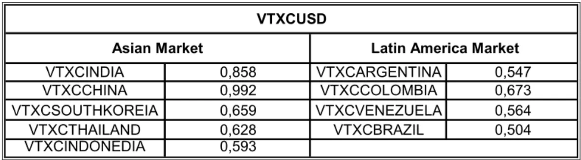
Concerning risk premium, they are negative with exception to India. This situation could be justified by the strong indexation of those economies to USD, like Table 4 ("Correlations between model variables and USD ") of this article shows, about 85,8%.

Analysing reserves variation, it is denoted that in the greater Asian economies, India, South Korea and China, there is a positively correlated with exchange rate variation (in India 36.5%, in South Korea 22.0% and in China 14.5%). These results are logical because the more euro appreciate, the greater the addition of competitiveness in those economies will be. So a bigger reserves variation will happen.

Table 3: Correlations between model variables (Latin America Market)

VRESARGENTINA -0,110 VRESCOLOMBIA -0,146 VRESVENEZUELA -0,174 VRESBRAZIL 0,032

VROARGENTINA 0,046 VRROCOLOMBIA -0,002 VROVENEZUELA 0,095 VROBRAZIL 0,150

VDTXJARGENTINA 0,520 VDTXJCOLOMBIA 0,121 VDTXJVENEZUELA 0,158 VDTXJBRAZIL 0,032

VTXCARGENTINA VTXCCOLOMBIA VTXCVENEZUELA VTXCBRAZIL

(10)

When we look at Table 3, we can verify that, in Latin America market, the interest rate difference variations are positively correlated with exchange rate variations, having a high significance in Argentina with 52,0%, and low significance in Brazil with 3,2%.

The risk premium variation is positive for all countries, except to Colombia. However, the result of 0,02% does not have any statistical meaning.

Concerning reserves variation, the correlations is negative, except to Brazil.

Table 4: Correlations between model variables and USD

VTXCINDIA 0,858 VTXCARGENTINA 0,547

VTXCCHINA 0,992 VTXCCOLOMBIA 0,673

VTXCSOUTHKOREIA 0,659 VTXCVENEZUELA 0,564

VTXCTHAILAND 0,628 VTXCBRAZIL 0,504

VTXCINDONEDIA 0,593

Latin America Market VTXCUSD

Asian Market

I

IIIII..11..22..EExxcchhaannggeerraatteeaauuttooccoorrrreellaattiioonnaannaallyyssiiss

We have done partial autocorrelation analysis to all exchange rate variations.

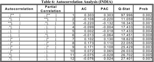
To exemplify partial autocorrelations, we select, inside the sample, the most significant economies such as India and China, whose results are transcribed in Table 5 and 6.

Table 5: Autocorrelation Analysis (CHINA)

A u to c o rre la tio n P a rtia l

C o rre la tio n A C P A C Q -S ta t P ro b . |** | . |** | 1 0 .3 1 6 0 .3 1 6 1 0 .7 1 8 0 .0 0 1 . |. | .*|. | 2 -0 .0 4 6 -0 .1 6 3 1 0 .9 5 0 0 .0 0 4 .*|. | . |. | 3 -0 .0 9 4 -0 .0 2 9 1 1 .9 1 2 0 .0 0 8 . |. | . |. | 4 0 .0 0 4 0 .0 4 6 1 1 .9 1 3 0 .0 1 8 . |. | . |. | 5 0 .0 4 8 0 .0 1 8 1 2 .1 6 7 0 .0 3 3 . |. | . |. | 6 0 .0 1 1 -0 .0 1 6 1 2 .1 8 1 0 .0 5 8 . |* | . |* | 7 0 .0 9 8 0 .1 2 6 1 3 .2 6 3 0 .0 6 6 . |* | . |* | 8 0 .1 5 2 0 .0 9 5 1 5 .9 2 9 0 .0 4 3 . |* | . |* | 9 0 .1 3 9 0 .0 7 8 1 8 .1 6 2 0 .0 3 3 . |* | . |* | 1 0 0 .1 1 7 0 .0 9 7 1 9 .7 7 6 0 .0 3 1 . |. | . |. | 1 1 0 .0 4 3 0 .0 1 3 2 0 .0 0 0 0 .0 4 5 . |. | . |. | 1 2 -0 .0 3 9 -0 .0 4 5 2 0 .1 8 5 0 .0 6 4

(11)

11

Table 6: Autocorrelation Analysis (INDIA)

A u to c o rre la tio n P a rtia l

C o rre la tio n A C P A C Q -S ta t P ro b . |** | . |** | 1 0 .3 0 3 0 .3 0 3 9 7 .9 9 6 0 .0 0 2 .*|. | **|. | 2 -0 .1 0 8 -0 .2 2 0 1 1 .0 5 9 0 .0 0 4 **|. | .*|. | 3 -0 .2 2 0 -0 .1 3 2 1 6 .3 4 3 0 .0 0 1 .*|. | . |. | 4 -0 .0 9 9 -0 .0 0 4 1 7 .4 3 3 0 .0 0 2 . |. | . |. | 5 0 .0 0 2 -0 .0 1 8 1 7 .4 3 3 0 .0 0 4 . |. | .*|. | 6 -0 .0 1 3 -0 .0 6 4 1 7 .4 5 1 0 .0 0 8 . |* | . |* | 7 0 .1 0 2 0 .1 3 0 1 8 .6 2 3 0 .0 0 9 . |* | . |* | 8 0 .1 7 3 0 .1 1 0 2 2 .0 5 5 0 .0 0 5 . |* | . |* | 9 0 .1 7 1 0 .1 0 8 2 5 .4 2 9 0 .0 0 3 . |* | . |. | 1 0 0 .0 7 2 0 .0 6 5 2 6 .0 3 3 0 .0 0 4 .*|. | . |. | 1 1 -0 .0 7 5 -0 .0 2 8 2 6 .7 0 2 0 .0 0 5 .*|. | . |. | 1 2 -0 .0 7 6 0 .0 2 4 2 7 .4 0 1 0 .0 0 7

Seeing partial autocorrelation values using Akaike Criterion (1974) [10], we verify that a first or second order model is enough to extract the autocorrelation problems.

I

IIIII..22..SSeerriieessSSttaattiioonnaarriittyyAAnnaallyyssiiss

We applied ADF (1979) [9, 15] and Philips-Perron (1988) [11] tests to certify series stationarity. Analysing Table 7, that presents principal results, we verify that statistics t allows us to reject unit root for any one of the usual significance levels. So being, a cointegration analysis is not necessary because variables are stationary.

Table 7: Exchange Rate Stationarity Analysis

1% level 5% level 1% level 5% level

ARGENTINA -3.534.868 -2.906.923 -5.526.994 -3.534.868 -2.906.923 -6.992.783 BRAzIL -3.495.021 -2.889.753 -8.254.211 -3.495.021 -2.889.753 -8.346.096 CHINA -3.495.021 -2.889.753 -7.312.393 -3.495.021 -2.889.753 -7.109.193 COLOMBIA -3.495.677 -2.890.037 -6.795.636 -3.495.021 -2.889.753 -5.992.426 SOUTH KOREIA -3.495.021 -2.889.753 -7.355.312 -3.495.021 -2.889.753 -7.188.940 INDIA -3.495.677 -2.890.037 -7.493.643 -3.495.021 -2.889.753 -7.146.495 INDONESIA -3.495.677 -2.890.037 -8.770.788 -3.495.021 -2.889.753 -7.631.215 THAILAND -3.495.677 -2.890.037 -7.732.378 -3.495.021 -2.889.753 -6.560.339 VENEZUELA -3.495.021 -2.889.753 -8.179.642 -3.495.021 -2.889.753 -8.149.298 Variable

Augmented Dickey-Fuller test statistic Phillips-Perron test statistic Test critical values:

Adj. t-Stat Test critical values:

t-Statistic

(12)

I

IIIII..33..MMaarrkkeettMMiiccrroossttrruuccttuurreeMMooddeellEEssttiimmaattiioonnRReessuullttss

We tested the Market Microstructure Model, according theoretical concerns already presented in introductory point of this paper, to Asian and Latin America markets.

The results were summarized in Table 8 (Asian countries estimation), and in Table 9 (Latin America countries estimation), with an OLS estimation.

For a ARCH/GARCH-M estimation methodology, the results are expressed in Table 10 (Asian countries estimation) and in Table 11 (Latin America countries estimation).

I

IIIII..33..11..OOLLSS

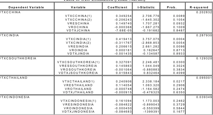
Table 8: OLS Estimation (Asian Market)

D e p e n d e n t V a r i a b l e V a r i a b l e C o e f f ic i e n t t - S t a t i s t i c P r o b . R - s q u a r e d V T X C C H I N A 0 . 2 0 2 8 3 2 V T X C C H IN A ( 1 ) 0 . 3 4 9 2 5 4 2 . 7 0 6 . 7 7 6 0 . 0 0 8 9 V T X C C H IN A ( 2 ) - 0 . 2 0 6 2 4 3 - 1 . 6 4 5 . 3 0 2 0 . 1 0 5 4 V R E S C H I N A 0 . 1 4 9 7 4 0 1 . 7 0 7 . 2 8 1 0 . 0 9 3 2 V R O C H I N A - 0 . 0 0 0 3 6 8 - 1 . 6 6 7 . 2 7 5 0 . 1 0 0 9 V D T X J C H I N A - 7 . 6 8 E - 0 5 - 0 . 1 9 1 6 8 2 0 . 8 4 8 7 V T X C I N D I A 0 . 2 8 7 9 3 0 V T X C I N D I A ( 1 ) 0 . 4 1 9 4 1 3 3 . 7 5 7 . 0 7 5 0 . 0 0 0 4 V T X C I N D I A ( 2 ) - 0 . 3 1 1 7 6 7 - 2 . 8 6 8 . 8 5 3 0 . 0 0 5 4 V R E S I N D I A 0 . 2 0 6 6 1 5 2 . 6 6 1 . 2 8 2 0 . 0 0 9 6 V R O I N D I A 0 . 0 0 0 1 8 1 0 . 1 6 2 6 4 7 0 . 8 7 1 3 V D T X J I N D I A - 0 . 0 0 1 4 3 5 - 0 . 1 3 4 5 8 7 0 . 8 9 3 3 V T X C S O U T H K O R E I A 0 . 1 2 9 3 2 0 V T X C S O U T H K O R E I A ( 1 ) 0 . 3 2 7 0 9 1 2 . 2 4 6 . 4 8 1 0 . 0 3 0 0 V R E S S O U T H K O R E I A 0 . 1 4 5 8 6 3 1 . 0 4 4 . 0 4 9 0 . 3 0 2 4 V R O S O U T H K O R E IA - 0 . 0 0 1 0 6 4 - 0 . 8 8 0 8 8 3 0 . 3 8 3 4 V D T X J S O U T H K O R E I A 0 . 0 1 5 8 4 3 0 . 8 3 2 4 6 4 0 . 4 0 9 9 V T X C T H A I L A N D 0 . 0 9 5 0 0 1 V T X C T H A IL A N D 1 ) 0 . 2 4 0 9 0 6 2 . 3 3 8 . 1 8 4 0 . 0 2 1 7 V R E S T H A I L A N D 0 . 1 1 4 0 5 4 1 . 0 6 3 . 3 2 0 0 . 2 9 0 6 V R O T H A IL A N D - 0 . 0 0 0 7 4 8 - 1 . 1 6 4 . 5 8 2 0 . 2 4 7 4 V D T X J T H A I L A N D - 0 . 0 0 0 9 1 5 - 0 . 4 7 6 3 2 5 0 . 6 3 5 0 V T X C I N D O N E S I A 0 . 0 3 9 3 4 9 V T X C I N D O N E S I A ( 1 ) 0 . 1 6 1 0 9 4 1 . 1 7 3 . 0 0 3 0 . 2 4 6 2 V R E S I N D O N E S I A - 0 . 0 8 4 8 2 2 - 0 . 8 9 9 0 4 3 0 . 3 7 2 9 V R O I N D O N E S I A - 0 . 0 0 0 4 5 0 - 0 . 5 5 0 3 9 9 0 . 5 8 4 4 V D T X J IN D O N E S I A - 0 . 0 8 4 6 8 3 - 1 3 9 9 3 9 1 0 . 1 6 7 7

Related to Asian market we verify that in the case of China and India, the adjustment is statistically significant, presenting an R2 of 20,28% for China and 28.79% for India. In the remaining countries, the model explicative capacity is very low. In the particular case of India, South Korea and China, we verify that euro appreciation is positively correlated with an increase of reserves in those countries, translating a competitiveness increase of those economies face to euro zone.

We still verify that risk premium variable is not statistically significant in exchange rate variations face to euro. To point out that risk premium being negative, except to India, opposes what it would be to expect. This question can be explained due to the USD strong indexation (see Table 4 of this paper).

(13)

13

Table 9: OLS Estimation (Latin America Market)

D e p e n d e n t V a ria b le V a ria b le C o e ffic ie n t t-S ta tis tic P ro b . R -s q u a re d

V T X C A R G E N T IN A 0 .4 8 8 9 8 4 V T X C A R G E N T IN A (1 ) 0 .5 4 6 6 3 8 3 .9 8 9 .8 8 7 0 .0 0 0 2 V T X C A R G E N T IN A (2 ) -0 .1 6 1 2 6 5 -0 .9 5 4 7 5 5 0 .3 4 3 6 V R E S A R G E N T IN A -0 .0 0 5 1 5 5 -0 .3 5 1 2 6 1 0 .7 2 6 6 V R O A R G E N T IN A -0 .0 0 1 0 5 7 -0 .5 9 7 2 8 8 0 .5 5 2 6 V D T X J A R G E N T IN A 0 .0 5 1 7 4 0 3 .3 9 2 .0 6 0 0 .0 0 1 2 V T X C C O L O M B IA 0 .2 5 7 2 3 1 V T X C C O L O M B IA (1 ) 0 .5 6 7 9 1 0 5 .0 5 3 .0 4 4 0 .0 0 0 0 V T X C C O L O M B IA (2 ) -0 .2 7 8 7 9 8 -2 .4 4 0 .3 7 6 0 .0 1 7 0 V R E S C O L O M B IA -0 .0 9 3 5 8 5 -0 .6 8 1 4 5 3 0 .4 9 7 7 V R R O C O L O M B IA -0 .0 0 0 8 2 3 -0 .3 1 8 8 0 7 0 .7 5 0 8 V D T X J C O L O M B IA 0 .0 5 8 6 6 0 1 .5 2 9 .1 9 2 0 .1 3 0 4 V T X C V E N E Z U E L A 0 .0 3 1 3 3 4 V T X C V E N E Z U E L A (1 ) 0 .2 7 4 2 3 4 2 .6 7 4 .8 7 1 0 .0 0 8 9 V R E S V E N E Z U E L A -0 .0 7 2 7 6 7 -0 .5 6 1 7 9 8 0 .5 7 5 7 V R O V E N E Z U E L A 0 .0 0 2 0 2 8 0 .9 1 8 6 4 8 0 .3 6 0 8 V D T X J V E N E Z U E L A 0 .0 7 1 3 9 7 1 .3 5 0 .0 9 9 0 .1 8 0 5 V T X C B R A Z IL 0 .1 5 6 5 2 8 V T X C B R A Z IL (1 ) 0 .3 8 1 2 4 6 3 .5 7 6 .9 5 2 0 .0 0 0 6 V R E S B R A Z IL 0 .0 3 8 4 2 3 0 .5 1 2 0 3 7 0 .6 1 0 1 V R O B R A Z IL 0 .0 0 4 0 9 5 0 .9 3 7 3 2 7 0 .3 5 1 6 V D T X J B R A Z IL 0 .0 4 0 9 0 8 0 .4 7 4 0 5 4 0 .6 3 6 8

Concerning Latin America market, specifically in Argentina and Colombia cases, the adjustment is statistically very strong with a R2 of 48,89%, in the case of Argentina, and 25.72% in the case of Colombia. In the remaining countries, model explicative capacity is very low, specially in the case of Venezuela.

Reserves variation is negative except to Brazil, however, it is not statistically significant.

We still verify that risk premium is not significant. As we confirmed in the correlation analysis, the risk premium is positive in Brazil, Venezuela and Argentina (more significant countries of Latin America market). Although the regression coefficient for the risk premium in Argentina is negative, translating a multicolinearity problem between the variables.

This relation with risk premium could be explained, on the one hand, due to a lesser correlation of those countries currencies face to euro and, on the other hand, to a greater political risk presented in macroeconomics variables.

In Argentina case, we verify that interest rate differential variation is statistically significant. Comparing our results with Medeiros’s (2005) [5] results, first we must take care of the following situations: Medeiros (2005) [5] only tested the Brazilian market face to USD, translating a different perspective from this study, that is face to euro. Medeiros’s (2005) [5] study got a R2 of 16%, being very similar to what we found for the same market, 15,65%; differently of our study, the risk premium variation coefficient is very significant in Medeiros (2005) [5] model presenting a value of 758%. This confirms what we have already said about the strong correlation between this country and USD.

(14)

I

IIIII..33..22..AARRCCHH//GGAARRCCHH--MM

Using GARCH-M methodology we improved clearly model explicative capacity for both markets, except for Thailand and Brazil.

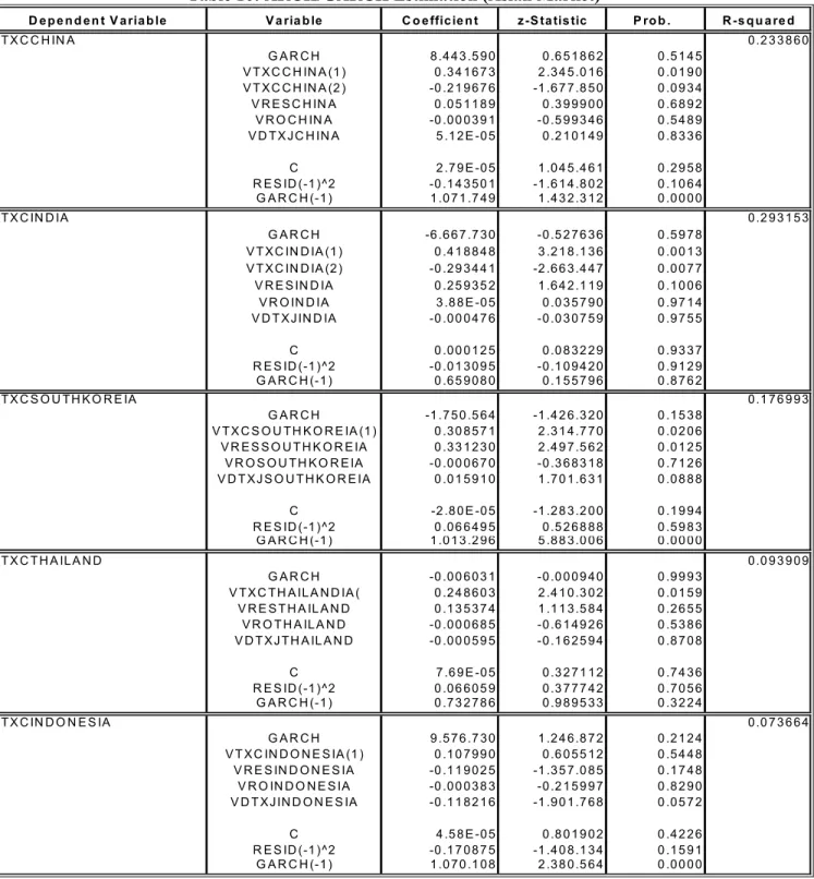
Table 10: ARCH/GARCH Estimation (Asian Market)

D e p e n d e n t V a ria b le V a ria b le C o e ffic ie n t z -S ta tis tic P ro b . R -s q u a re d

V T X C C H IN A 0 .2 3 3 8 6 0 G A R C H 8 .4 4 3 .5 9 0 0 .6 5 1 8 6 2 0 .5 1 4 5 V T X C C H IN A (1 ) 0 .3 4 1 6 7 3 2 .3 4 5 .0 1 6 0 .0 1 9 0 V T X C C H IN A (2 ) -0 .2 1 9 6 7 6 -1 .6 7 7 .8 5 0 0 .0 9 3 4 V R E S C H IN A 0 .0 5 1 1 8 9 0 .3 9 9 9 0 0 0 .6 8 9 2 V R O C H IN A -0 .0 0 0 3 9 1 -0 .5 9 9 3 4 6 0 .5 4 8 9 V D T X J C H IN A 5 .1 2 E -0 5 0 .2 1 0 1 4 9 0 .8 3 3 6 C 2 .7 9 E -0 5 1 .0 4 5 .4 6 1 0 .2 9 5 8 R E S ID (-1 )^2 -0 .1 4 3 5 0 1 -1 .6 1 4 .8 0 2 0 .1 0 6 4 G A R C H (-1 ) 1 .0 7 1 .7 4 9 1 .4 3 2 .3 1 2 0 .0 0 0 0 V T X C IN D IA 0 .2 9 3 1 5 3 G A R C H -6 .6 6 7 .7 3 0 -0 .5 2 7 6 3 6 0 .5 9 7 8 V T X C IN D IA (1 ) 0 .4 1 8 8 4 8 3 .2 1 8 .1 3 6 0 .0 0 1 3 V T X C IN D IA (2 ) -0 .2 9 3 4 4 1 -2 .6 6 3 .4 4 7 0 .0 0 7 7 V R E S IN D IA 0 .2 5 9 3 5 2 1 .6 4 2 .1 1 9 0 .1 0 0 6 V R O IN D IA 3 .8 8 E -0 5 0 .0 3 5 7 9 0 0 .9 7 1 4 V D T X J IN D IA -0 .0 0 0 4 7 6 -0 .0 3 0 7 5 9 0 .9 7 5 5 C 0 .0 0 0 1 2 5 0 .0 8 3 2 2 9 0 .9 3 3 7 R E S ID (-1 )^2 -0 .0 1 3 0 9 5 -0 .1 0 9 4 2 0 0 .9 1 2 9 G A R C H (-1 ) 0 .6 5 9 0 8 0 0 .1 5 5 7 9 6 0 .8 7 6 2 V T X C S O U T H K O R E IA 0 .1 7 6 9 9 3 G A R C H -1 .7 5 0 .5 6 4 -1 .4 2 6 .3 2 0 0 .1 5 3 8 V T X C S O U T H K O R E IA (1 ) 0 .3 0 8 5 7 1 2 .3 1 4 .7 7 0 0 .0 2 0 6 V R E S S O U T H K O R E IA 0 .3 3 1 2 3 0 2 .4 9 7 .5 6 2 0 .0 1 2 5 V R O S O U T H K O R E IA -0 .0 0 0 6 7 0 -0 .3 6 8 3 1 8 0 .7 1 2 6 V D T X J S O U T H K O R E IA 0 .0 1 5 9 1 0 1 .7 0 1 .6 3 1 0 .0 8 8 8 C -2 .8 0 E -0 5 -1 .2 8 3 .2 0 0 0 .1 9 9 4 R E S ID (-1 )^2 0 .0 6 6 4 9 5 0 .5 2 6 8 8 8 0 .5 9 8 3 G A R C H (-1 ) 1 .0 1 3 .2 9 6 5 .8 8 3 .0 0 6 0 .0 0 0 0 V T X C T H A IL A N D 0 .0 9 3 9 0 9 G A R C H -0 .0 0 6 0 3 1 -0 .0 0 0 9 4 0 0 .9 9 9 3 V T X C T H A IL A N D IA ( 0 .2 4 8 6 0 3 2 .4 1 0 .3 0 2 0 .0 1 5 9 V R E S T H A IL A N D 0 .1 3 5 3 7 4 1 .1 1 3 .5 8 4 0 .2 6 5 5 V R O T H A IL A N D -0 .0 0 0 6 8 5 -0 .6 1 4 9 2 6 0 .5 3 8 6 V D T X J T H A IL A N D -0 .0 0 0 5 9 5 -0 .1 6 2 5 9 4 0 .8 7 0 8 C 7 .6 9 E -0 5 0 .3 2 7 1 1 2 0 .7 4 3 6 R E S ID (-1 )^2 0 .0 6 6 0 5 9 0 .3 7 7 7 4 2 0 .7 0 5 6 G A R C H (-1 ) 0 .7 3 2 7 8 6 0 .9 8 9 5 3 3 0 .3 2 2 4 V T X C IN D O N E S IA 0 .0 7 3 6 6 4 G A R C H 9 .5 7 6 .7 3 0 1 .2 4 6 .8 7 2 0 .2 1 2 4 V T X C IN D O N E S IA (1 ) 0 .1 0 7 9 9 0 0 .6 0 5 5 1 2 0 .5 4 4 8 V R E S IN D O N E S IA -0 .1 1 9 0 2 5 -1 .3 5 7 .0 8 5 0 .1 7 4 8 V R O IN D O N E S IA -0 .0 0 0 3 8 3 -0 .2 1 5 9 9 7 0 .8 2 9 0 V D T X J IN D O N E S IA -0 .1 1 8 2 1 6 -1 .9 0 1 .7 6 8 0 .0 5 7 2 C 4 .5 8 E -0 5 0 .8 0 1 9 0 2 0 .4 2 2 6 R E S ID (-1 )^2 -0 .1 7 0 8 7 5 -1 .4 0 8 .1 3 4 0 .1 5 9 1 G A R C H (-1 ) 1 .0 7 0 .1 0 8 2 .3 8 0 .5 6 4 0 .0 0 0 0

(15)

15

Analysing Asian market results, we can verify a significant improvement in model adjustment. In fact results show that,

- Indonesia passed from a R2 of 3,9% to 7,36%;

- South Korea passed from a R2 of 12,93% to 17,69%; and - China passed from a R2 of 20,28% to 23,38%.

We also verify that risk premium variation is negative, except for India, although no showing significance for any one of the selected countries inside this market.

Only Indonesia interest rate variation reveals to be significant, even opposing what it would be expect (to see correlation face to USD).

Table 11: Modelação por ML - ARCH (Latin America Market)

D e p e n d e n t V a r ia b le V a r ia b le C o e ff ic ie n t z - S t a t is t ic P r o b . R - s q u a r e d V T X C A R G E N T IN A 0 .5 1 9 5 7 3 G A R C H 1 .1 8 5 .4 8 0 2 .1 4 2 .9 7 0 0 .0 3 2 1 V T X C A R G E N T IN A (1 ) 0 .5 1 2 7 6 6 5 .0 8 2 .9 6 8 0 .0 0 0 0 V T X C A R G E N T IN A (2 ) -0 .1 4 3 5 8 9 - 0 .9 9 6 4 5 4 0 .3 1 9 0 V R E S A R G E N T IN A -0 .0 1 0 5 0 3 - 0 .5 2 7 1 2 4 0 .5 9 8 1 V R O A R G E N T IN A -0 .0 0 0 4 9 7 - 0 .3 4 1 2 5 3 0 .7 3 2 9 V D T X J A R G E N T IN A 0 .0 4 1 6 0 6 4 .5 6 5 .4 1 0 0 .0 0 0 0 C -2 .0 0 E -0 5 -1 .4 5 9 .4 1 8 0 .1 4 4 5 R E S ID (- 1 )^ 2 -0 .0 0 1 7 3 8 - 0 .0 9 0 0 0 8 0 .9 2 8 3 G A R C H ( -1 ) 1 .0 2 0 .2 5 7 7 .0 3 0 .4 1 1 0 .0 0 0 0 V T X C C O L O M B IA 0 .2 8 2 2 4 1 G A R C H 7 .2 8 9 .5 8 2 1 .4 2 4 .5 6 7 0 .1 5 4 3 V T X C C O L O M B IA (1 ) 0 .5 5 0 1 6 3 5 .3 5 4 .9 3 4 0 .0 0 0 0 V T X C C O L O M B IA (2 ) -0 .3 3 7 5 7 5 -3 .4 7 3 .9 4 6 0 .0 0 0 5 V R E S C O L O M B IA -0 .1 8 7 2 2 4 -1 .3 4 1 .9 5 8 0 .1 7 9 6 V R R O C O L O M B IA -0 .0 0 0 4 1 5 - 0 .1 8 1 3 6 5 0 .8 5 6 1 V D T X J C O L O M B IA 0 .0 5 9 8 8 6 1 .7 7 6 .3 2 1 0 .0 7 5 7 C 1 .3 6 E -0 5 0 .5 9 3 0 5 7 0 .5 5 3 1 R E S ID (- 1 )^ 2 -0 .0 5 7 7 3 9 -1 .9 2 7 .1 0 5 0 .0 5 4 0 G A R C H ( -1 ) 1 .0 4 9 .7 0 9 1 .4 4 2 .0 5 6 0 .0 0 0 0 V T X C V E N E Z U E L A 0 .0 3 7 8 8 0 G A R C H 0 .8 7 5 6 3 7 0 .8 8 6 5 3 3 0 .3 7 5 3 V T X C V E N E Z U E L A ( 1 ) 0 .3 6 1 3 1 9 1 .1 4 9 .7 2 4 0 .0 0 0 0 V R E S V E N E Z U E L A 0 .1 0 8 4 2 9 1 .7 6 7 .8 2 8 0 .0 7 7 1 V R O V E N E Z U E L A 0 .0 0 0 5 7 5 0 .4 4 7 1 2 7 0 .6 5 4 8 V D T X J V E N E Z U E L A 0 .0 6 5 9 9 5 2 .3 5 6 .4 4 2 0 .0 1 8 5 C 0 .0 0 0 3 2 0 1 .9 8 9 .9 1 8 0 .0 4 6 6 R E S ID (- 1 )^ 2 1 .2 0 1 .4 7 8 3 .6 6 7 .2 7 8 0 .0 0 0 2 G A R C H ( -1 ) 0 .1 2 9 0 7 7 1 .1 5 9 .0 4 7 0 .2 4 6 4 V T X C B R A Z IL 0 .1 4 5 5 3 8 G A R C H 0 .9 2 9 4 2 3 0 .3 3 4 0 3 3 0 .7 3 8 4 V T X C B R A Z IL (1 ) 0 .2 6 0 0 0 3 3 .0 7 9 .6 1 7 0 .0 0 2 1 V R E S B R A Z IL -0 .0 0 1 8 4 7 - 0 .0 3 0 0 3 2 0 .9 7 6 0 V R O B R A Z IL 0 .0 0 5 9 1 0 1 8 8 3 0 4 2 0 .0 5 9 7 V D T X J B R A Z IL 0 .0 2 6 0 9 6 0 .3 1 5 9 8 1 0 .7 5 2 0 C 6 .2 4 E -0 5 0 .4 6 3 3 8 9 0 .6 4 3 1 R E S ID (- 1 )^ 2 0 .2 6 3 4 5 4 1 .7 0 3 .8 0 9 0 .0 8 8 4 G A R C H ( -1 ) 0 .7 1 4 5 9 0 4 .7 3 8 .2 6 8 0 .0 0 0 0

(16)

The multicolinearity problem remains for Argentina risk premium, being the other results similar to the OLS estimation.

To enhance that, in Argentina, Colombia and Venezuela, the interest rate difference variation is statistically significant to 5% level for Argentina and Venezuela, and for 10% significance level for Colombia. This fact shows that those countries have a greater difference variation face to euro originated by the biggest inflating risk, so creating a bigger perception of the market to the risk premium of those countries.

Our results show that ARCH/GARCH-M modulation improved model explicative capacity, confirming Medeiros (2005) [5] results, where this methodology find more robust results.

IV – CONCLUSION

Following Medeiros (2005) [5] study about country risk premium importance in exchange rate variation comprehension, we tested market microstructure model for Asian and Latin America market, face to Europe.

We selected the most significant economies for each market between 1999 the 2007. For Asia, we studied China, India, South Korea, Indonesia and Thailand. For Latin America, we studied Brazil, Argentina, Venezuela and Colombia. For the mentioned countries we collected monthly samples for the model variables: exchange rate, reserves, interest rate and consumer price index. Risk premium was calculated according with Thayer Watkins (2005) [7].

In its study, Medeiros (2005) [5] analyzed the Brazilian market face to USD. To do that, Medeiros (2005) [5] measure transactions flow using the daily balance between USD sell and USD purchase offers in Brazilian market. In our study we treated this question differently: we used total reserves for each mentioned country. Medeiros (2005) [5] used Brazilian daily risk premium, while we calculated risk premium according with Thayer Watkins (2005) [7]. So, to establish comparations between results, we have to attempt to these differences.

We verified that, in our study, the market microstructure model has a strong explicative capacity in Latin America countries instead of the Asian countries (in both modulations, OLS [14] and ARCH/GARCH-M [12, 13, 16, 17, 18, 19, 20, 21]).

Risk premium variations are negatively correlated with exchange rate variation for Asian market (except for India), and positively correlated with Latin America countries (except for Colombia).

As we verified in ARCH/GARCH-M model, the interest rate differential variation is statistically significant in exchange rate variation explanation (except for Brazil). These results confirm that risk premium is important, denoting bigger risks in interest rate variation. In the Asian case, the fact of risk

(17)

17

premium being negative, this can be explained due to the bigger correlation between these currencies face to USD, as we can see in the present study.

ARCH/GARCH-M modulation improved model explicative capacity, just like Medeiros (2005) [5] results. This fact denotes the biggest capacity of this model in catching non-linearity relations between variables.

The present paper presents obviously limitations: in sample dimension terms (euro only started to formally exist in 1999), and in our capacity in calculating risk premium indirectly.

So, it will be interesting to apply and study more deeply market microstructure models, using non- linear modulations.

(18)

B

BIIBBLLIIOOGGRRAAFFIICCRREEFFEERREENNCCEESS

[1] Cassel, Gustav (1916), “The Present Situation in Foreign Exchanges”, Economic Journal, pp. 62-65.

[2] Cassel, Gustav (1918), “Abnormal Deviations in International Exchanges”, Economic Journal, 28, pp. 413-415.

[3] Evans, M.D.D. and Lyons, R.K. (2002), “Order Flow and Exchange Rate Dynamics”, Journal of Political Economy, 110(1): 170-180.

[4] O’Hara, M. (1995), “Market Microstructure Theory”, Cambridge, MA: Blackwell Business, 1995.

[5] Medeiros, Otavio R. (2005), “Exchange Rate and Market Microstructure in Brazil”, Academic Open Internet Jounal, volume 14.

[6] Macdonald, R. and Taylor, M.P. (1992), “Exchange Rate Economics: A Survey”, IMF Staff Papers, March 1992.

[7] Watkins, Thayer (2005), “Country Risk Premiums”, San Jose State University, Economics Department.

[8] Famma, Eugene (1984), “Forward and Sopt Exchange Rates”, Journal of Monetary Economics, 14, 319-338.

[9] Dickey, D.A. and Fuller, W.A. (1979), “Distribution of Estimators for Time Series Regressions with a Unit Root”, Journal of the American Statistical Association 74, 427-31.

[10] Akaike, Hirotugu (1974), “A new look at the statistical model identification”, IEEE Transactions Automatic Control 19 (6): 716-723.

[11] P. Perron (1988) “Trends and random walks in macroeconomic time series”, Journal of Economic Dynamics and Control 12, 297–332.

(19)

19

[12] Bollerslev, T. (1986), "Generalized Autoregressive Conditional Heteroscedasticity", Journal of Econometrics 31, pp. 373-399.

[13] Bollerslev, T. (1987), " A Conditionaly Heteroskedastic Time Series Model For Speculative Prices and Rates of Return ", Review of Economics and Statistics 69, pp. 542-547.

[14] Box, G. and. P. & G.M. Jenkins (1976), “Time-Series Analysis , Forecasting and Control”, S. Francisco Holden-Day ( ed. 1976 ).

[15] Dickey, D. A. and W. A. Fuller (1981), " Likelihood Ratio Statistics For Autoregressive Time Series With a Unit Root ", Econometrica 49, pp. 1057-1072.

[16] Engle, R. F. (1982), " Autoregressive Conditional Heteroscedasticity With Estimates of The Variance of U. K. Inflation ", Econometrica 50, pp. 987-1008.

[17] Engle, R. F. and T. Bollerslev (1986), " Modelling The Persistence of Conditional Variances ", Econometric Reviews 5, pp. 1-50.

[18] Engle, R. F. and G. González-Rivera (1991), " Semiparametric ARCH Models ", Journal of Business & Economic Statistics 9, pp. 345-359.

[19] Hsieh, D. A. (1989), " Modelling Heteroskedasticity in Daily Foreign Exchange Rate Changes ", Journal of Business 62, pp. 339-368.

[20] Lamoureux, C.G. e W. D. Lastrapes (1990), " Persistence in Variance , Structural Change and The GARCH Model ", Journal of Business & Economic Statistics 8, pp. 225- 234.

[21] Nelson, D.B. (1991), " Conditional Heteroskedasticity in Asset Returns : A New Approach", Econometrica 59, pp. 347-370.

(20)

CIGE – Centro de Investigação em Gestão e Economia Universidade Portucalense – Infante D. Henrique

Rua Dr. António Bernardino de Almeida, 541/619 4200-072 PORTO PORTUGAL http://www.upt.pt dcee@uportu.pt ISSN 1646-8953