A Work Project, presented as part of the requirements for the Award of a Master Degree in Economics from the NOVA- School of Business and Economics
The effects of overconfidence in job market
signaling- an experimental approach
Rita Alexandra Gouveia da Silva (30033)
A Project carried out on the Master in Economics Program, under the supervision of: Professor Alexander Coutts
THE EFFECTS OF OVERCONFIDENCE IN JOB MARKET SIGNALING - AN EXPERIMENTAL APPROACH
Abstract
The job market works under asymmetric information, making it hard for firms to know the real capabilities of the workers they hire. Workers can help overcome this asymmetry by signaling their productivity with investments in education. However, it’s fair to assume that workers sometimes miscalculate their own abilities, which disturbs the functioning of the signal. This study intends to analyze the effects of overconfidence amongst workers on the various parameters of the game by conducting an experiment. The results from the experiment suggest that the profits of both workers and firms will be greatly impaired as a consequence.
Acknowledgments
I would like to express my sincere gratitude to everyone that helped me through the completion of this degree. To my advisor, Professor Alexander Coutts, for his endless help and guidance. To my mom, dad, and Joana, for always making me believe it was possible. To my grandparents, aunt Elsa, godfather, and Rodrigo, for being my home away from home. Finally, to everyone who kindly gave me some of their time answering my surveys.
I. Introduction
It is important to understand how markets work with asymmetric information because in reality it’s very common that one side of a market has more information than another. One of the classic asymmetric information problems studied in economics is the Spence signaling model, Spence (1973). In this paper Spence described a stylized example of workers with private information about their ability or productivity, trying to signal their productivity to firms who compete to hire them. Education can work as a signal that workers send to employers to indicate their productivity. Since a worker’s productivity can only be observed after the employer has already hired him, they must rely on those signs to predict which salary will be the most appropriate for a worker. For the signaling model to work, there has to be a negative relationship between the marginal productivity of the worker and his cost for sending the signal. In the context of education, it means that the less productive a worker is, the more costly it will be for him to obtain an education. This should ensure that highly productive workers get more education than low productivity workers and that low productivity workers do not find it profitable to imitate high productivity workers.
Since there is not very much evidence about the signaling model, and evidence from behavioral and experimental economics suggests that people don’t always behave according to theory, I believe it is worth reflecting on how people evaluate their own abilities. If they, in fact, misevaluate them, this can lead to biases such as overconfidence. In the case of the signaling model, this means that some workers may believe they are high types, when in fact they are low types. This leads us to the following questions: Are all low productive workers aware of their limitations? Do firms also perceive that workers can be overconfident? How does this affect the equilibrium?
As has been shown by numerous papers in the field of behavioral economics, it is true that our choices as rational economic agents are often compromised by optimism and overconfidence.
In this context, being overconfident means that one is optimistic about his ability. Overconfidence is then present when low productive workers believe they are highly productive workers, meaning they’ll behave and make choices taking into consideration lower costs than their real ones. My goal is to see the implications of this in various aspects of the signaling game, namely in the pooling and separating equilibria. In theory, in the pooling equilibrium workers, independently of their type, earn their average worth when everyone chooses not to send the signal. In the separating equilibrium, the optimal is for workers to earn exactly their worth when highly productive workers choose to send the signal and low productive workers choose to not send the signal.
To do so, I conducted an online experiment, designed to observe the following:
- Which salary, high or low, are employers willing to offer a worker if they observe his education, knowing that there’s a possibility that some workers are overconfident regarding their own capabilities;
- Which level of education will workers choose, knowing which salary each level of education earns;
- What proportion of types (low productive workers to high productive workers) are being assumed by employers and how do these compare to reality;
- How do workers perceive their chance of being very productive;
- What are the final outcomes for the employers and the workers given their choices, and how do these compare to the equilibrium outcomes in the original model.
For the experiment, I conducted two distinct surveys: one from the employers’ perspective and one from the workers’ perspective. In both surveys, the setup is the same, in which there are two firms competing to hire one worker. The employers’ survey asks questions regarding the
wage choice given the signal. The workers’ survey asks questions regarding the choice of sending, or not, the signal, depending on different wages.
II. Literature Review
The idea that one agent is trying to convey some information about himself to another agent is known as signaling. This concept is well-known in the economic context, and many authors have applied it to real life situations. Spence (1973, 1974) explored the notion in a job market setting, by explaining how workers use education to signal their abilities to firms. Investment in education in his model has no intrinsic productive value, but it does work as a signal. Firms distinguish highly productive workers as being the ones who invest in education the most because they assume that it costs them less than it does to the lower productive types. Workers who invest the most are then rewarded with higher wages. My analysis will take place in this context. To make matters simpler, I will, however, consider specific values for the different variables, while Spence focused on keeping his theory more general.
Most research regarding this model has been theoretical. However, as it deals with real-life decisions, experiments on the subject are indispensable. Unfortunately, there are almost no experiments on signaling. Kubler et al. (2008) study both a signaling and a screening variant of the Spence education model and analyze the effect of having three employers instead of two. Their experiment confirmed that the most efficient type of worker chose the more costly investment more frequently and therefore received significantly higher wages than those who didn’t invest. However, they also concluded that the payoffs for the highly efficient workers ended up not being that higher than those of investing workers. This is likely due to non-investing workers’ wages being too high compared to the theoretical prediction. In the employers’ perspective, it was seen that they earned higher profits when hiring an investing worker than when hiring a non-investing worker. The amount of costly investments is the same for signaling and screening, no matter how many employers are competing. It is important to
note that Kubler et al. (2008) manipulate the cost of the education investment, making it exogenous. In my experiment, I will allow for low and high types to arise endogenously. In their experiment, there is also a key assumption that workers fully know their ability. However, given evidence of overconfidence across many settings, in my setting it seems likely that when individuals are unaware of their competence, they will over-estimate it.
A number of studies in psychology suggest that the majority of people is prone to being overconfident about their capabilities and irrationally confident and optimistic about the future. Many authors have succeeded at showing this by conducting experiments in various contexts, thus proving the broadness of this bias. Svenson (1981) has one of the most known studies on the subject. He asked subjects about their performance as drivers and how it compared to other people’s. The conclusion was that people have a strong tendency to overestimate their abilities since the majority perceived themselves as being better and less risky at driving than the rest. In fact, an astonishing 93% of the subjects believed that they were better than the median, even if only 50% could really be.
Overconfidence arises when the event is seen as controllable and when subjects are engaged in the outcome. So, when the outcomes depended on the subjects’ abilities, people overestimate their chances of success (Weinstein and Neil (1980); Camerer and Lovallo (1990)). In the case of how workers perceive their own capabilities, overconfidence is then expected to be relevant because people have a feeling of controlling the situation since it’s their choice to invest, or not, in education. They are also highly emotionally invested in the outcome because it will directly influence an important part of their lives, their wages.
It’s already been established that people judge their abilities in a brighter light than they judge others’. But why does this happen? Kruger and Dunning (1999, 2002) suggest it’s because people who are unskilled are also less cognitively capable of perceiving this. This is the reason
people who are unskilled tend to overestimate their abilities much more than skilled people. This leads me to focus my analysis in the effects of overconfidence and not of under confidence. III. Theory and Predictions
The job market functions under various types of uncertainty. Workers and employers only get information about each other after hiring, and even that may take a lot of time. Following Spence (1973), I only consider the information asymmetry of employers not knowing how productive a worker is before hiring. Their goal is to offer a wage that corresponds to the worker’s marginal productivity, but since that’s not observable, employers must look for other indicators. These indicators are what we call “signals” and are individual’s observable attributes that can be controlled and changed by him (Jervis, 1970). Observing the signals, the employer can assign an expected marginal productivity for that individual. This translates to the offered wage, that workers can promptly observe.
The reason signals should effectively distinguish the type of workers is the assumption that marginal productivity and the cost of signaling are negatively correlated. Only like this can we assure that a higher signal corresponds to a more productive worker. In practice, in the case of education as a signal, this means that less productive people will have a higher cost of getting a certain level of education than high productive people. This is so because the cost of education isn’t only a monetary cost but also one of intellectual effort and time. Workers should then invest in education with consideration of their abilities, otherwise, they could miscalculate their costs.
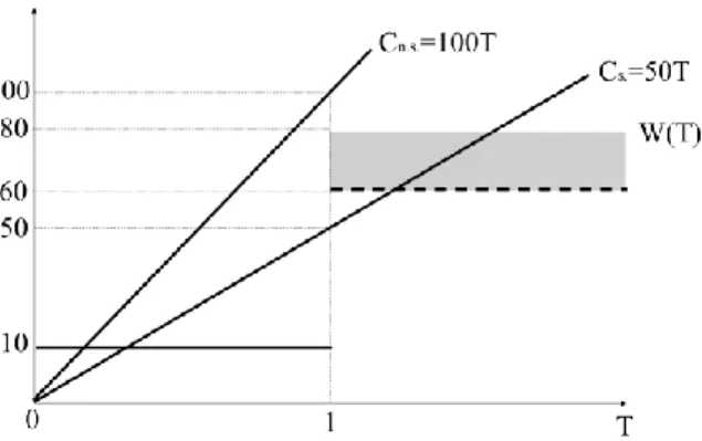
In the setup of my experiment, there are two firms and they are both Bertrand competing on offering wages to workers. These workers can only be of one of two types, with distinct marginal productivities. The first type, which we’ll denote by “not smart”, has a marginal productivity of 10 and the second type, which we’ll denominate by “smart”, has a marginal productivity of 80. In terms of proportion, we can say that q1 of the population is “not smart”
and 1-q1 is “smart”. To make things simpler, the signal will consist of taking a test, which can
be compared to getting a certain level of education. Taking the test will obviously imply a cost, that will be different depending on the type of worker. For a “not smart” worker the cost is Cn.s.=100€ per test (Cn.s.(T)=100T) and for a “smart” worker it will only be Cs.=50€ per test
(Cs.(T)=50T).
A perfect Bayesian equilibrium (PBE) is a set of strategies and beliefs that simultaneous satisfy the following conditions:
i. Sequential Rationality: All agents maximize their expected payoffs given their beliefs and considering everyone else’s strategies
ii. Bayes’ Rule: All agents’ beliefs are correct and are not contradicted
The strategies of the workers are to take the test or not to take the test, and their beliefs are about the wages that firms will offer to workers who take and not take the test. The strategies for the firms are to set wages for workers who take the test and for workers who don’t take the test, and their beliefs are about the probability that a worker is “not smart” if he takes the test and if he doesn’t take the test. The PBE in this context means that workers are optimally choosing T=0 or T=1. For firms, it means that they have correct beliefs1 about these decisions, and, since they are competing with each other for the worker, they offer wages equal to the workers’ expected productivity.
i. No Information: Before getting into the pure strategy equilibria, let’s look at the case when firms have no information about the workers.
In this context, this means that workers wouldn’t have the option to take the test. Firms would have to offer a wage equal to the expected productivity of the workers W=0,5*80+0,5*10=45. “Smart” and “not smart” workers would have a payoff of 45-0=45.
1 PBE says nothing about the firms’ beliefs in off-equilibrium path. Any belief that doesn’t interfere with the
There are then two types of possible pure strategy equilibria:
ii. Pooling Equilibria: Both types of workers choose the same action, to take the test or to not take the test. Firms pay them the average wage for they believe there’s a 50% chance they are “not smart” having chosen one of those actions.
Let’s start by considering the case in which all workers choose to take the test. The wage is equal to q1*10+(1-q1)*80=80-70q1. Since firms believe that there’s a 50% that these workers are “not smart”, they compute the average2 wage W=80-70*0,5=45. Figure 1 shows that the
optimal choice is for both groups to not take the test because the outcome will be more favorable for both if they choose T=0. Even for “smart” people, the profit of choosing T=1 will be 45-50=-5, and for choosing T=0 would be at worst 103-0=10. For “not smart” workers, getting the high wage doesn’t compensate for their costs because when they choose T=0 their payoff is at worst 10-0=10 and when they choose T=1 their payoff is 45-100=-55. This invalidates being a PBE because it doesn’t satisfy the first condition of sequential rationality: workers are better off switching their strategy regarding the firms’ actions.
2 Due to competition, the wage will be bid up to average productivity since this will equate to firms making zero
profit.
3 In the worst-case scenario firms believe a worker who doesn’t take the test is “not smart” with probability
one, thus paying the lowest wage possible, 10. Figure 1-Optimizing choices of number of tests for both types
When all workers choose to not take the test, the wage is again q1*10+(1-q1)*80=70q1. Firms maintain their belief that 50% of these workers are “not smart”, so W=45 again. For “smart” workers, the optimizing choices of number of tests show that the optimal choice is, in fact, T=0 since the profit of this choice will be 45-0=45 and of choosing T=1 would be 804-50=30, at best. For “not smart” workers T=0 is also the optimal decision because this has a profit of 45-0=45 and T=1 would get a profit of 80-100=-20. This set is a PBE because both conditions, sequential rationality and Bayes’ rule, are secured. This PBE actually holds regardless of the beliefs that firms have.
iii. Separating Equilibria: Different types of workers choose different actions. In this case, smart workers take the test and not smart workers don’t take the test, which allows form firms to know exactly who is who.
We start by having the employers’ beliefs that if T<T*, the probability of the worker being “not smart” is one, and if T≥T*, the probability of the worker being “smart” is one. Even though this variable will only take discrete amounts, I will treat it as continuous for the theoretical analysis.
4 In the best-case scenario firms believe a worker who takes the test is “smart” with probability one, thus
In figure 2, these conditional beliefs are represented, so we can see that for anyone taking T<T* the offered wage is 10 and for T≥T* is 80. Knowing this, “not smart” and “smart” workers will choose their optimal level of T. For anyone that chooses T<T*, the optimal decision is to take 0 tests, T=0, because only here can they maximize their outcome. For anyone that chooses T≥T*, the optimal decision is to take T=T* for the same reason. In figure 3, this reasoning is easily observed: the cost of taking the tests is increasing while the wages are fixed, so taking the minimum number of tests in that interval is always more profitable. The conditions that need to hold to confirm the employers’ beliefs are the following: “Not smart” people will choose T=0 if 10>80-Cn.s.T*Cn.s.>70/T* and “Smart” people will choose T=T* if
80-Cs.T*>10Cs.<70/T*. Combining the two, we see that the employer’s initial beliefs are
confirmed if Cn.s.>70and Cs.<70, since tests can only be taken a discrete amount of times, T*=1.
Figure 3-Optimizing choices of number of tests for both types Figure 2-Offered wages as a function of number of tests taken
The equilibrium signal, T*=1, works as a prerequisite for workers to get the high wage. However, the true productivity of someone isn’t acquired with the test itself. This means that it’s possible that someone attempts to do the test in order to get a high wage but isn’t in fact productive. If employers start to realize that not everyone that takes the test is a “smart” worker, their beliefs will change. They start to expect that if they observe T=0, the worker is “not smart” with probability 15, and if T=1, the worker is “not smart” with probability q1 and “smart” with
probability 1-q1. The wage for T=0 is still 10€ but the wage for T=1 is now q1
*10+(1-q1)*80=80-70q1. So, what beliefs should firms have in order for “smart” workers to still be
better off taking the test and for “not smart” workers to still be better off not taking the test?
Like it’s represented in figure 4, “Smart” workers will always prefer to choose T=1 as long as W(T=1)- Cs>W(T=0). Since W(T=0)=10 and Cs=50, this translates to W(T=1)>60. To find the
corresponding beliefs, 60=80-70q1q1=2/7q1<2/7. “Not smart” workers will rather choose T=0 if W(T=1)- Cn.s <W(T=0). Cn.s=100 so W(T=1)<110. The respective beliefs are
110=80-70q1q1=-3/7q1>-3/7. Considering that 10≤W(T=1)≤80 and q1≥0, and combining both types of workers conditions, we conclude that 0≤q1<2/7 and 60<W(T=1)≤80. Obviously, if W(T=1)=60 and q1=2/7, “smart” workers will be indifferent between taking the test or not.
5 Since the focus is overconfidence, we’ll disregard the possibility of relevant under confidence.
This means that the firms’ beliefs about the “not smart” workers need to be small enough so that the wages are high enough to assure it’s worth it for “smart” workers to choose T=1. In sum, without the possibility of taking the test the prediction is for firms to offer a wage equal to the average productivity of all workers W=45. A pooling equilibrium suggests that all workers choose T=0. Firms believe that workers are “not smart” with probability 0,5 and offer a wage of 45. A separating equilibrium suggests that “smart” workers choose T=1 and “not smart” workers choose T=0. Firms believe that if T=1 the worker is “not smart” with probability zero and if T=0 the worker is “not smart” with probability one. They offer a wage of 80 to workers who choose T=1 and a wage of 10 to the ones who choose T=0.
IV. Data
Two distinct surveys were designed for the experiment. The first one asked questions from the employers’ perspective. The main purpose was to see the wages people were willing to offer a worker considering i) they had no information about him; ii) they knew he had taken the test; iii) they knew he hadn’t taken the test. This survey had 23 respondents over the course of a week.
The second one asked questions from the workers’ perspective. The intention was to observe if people chose to take the test, or not, considering firms offered i) 80€ to workers who took the test and 10€ to workers who didn’t; ii) 42€ to workers who took the test and 25€ to workers who didn’t; iii) 75€ to workers who took the test and 15€ to workers who didn’t. The first set of wages were chosen because they make up for the separating equilibria. The employers’ survey was conducted first, and the second set of wages was retrieved from those answers. The final set was chosen because I figured it was interesting to see what “smart” workers, in particular, chose since they should be indifferent. I also took the opportunity to see the expectations subjects had regarding how much firms offered to a worker who took the test and to a worker who didn’t. This survey had 50 respondents over the course of a week. In order to
be able to detect the effects of overconfidence from workers, workers were oversampled relative to employers.
Even though the surveys served very distinct purposes, they also had a lot of parts in common. Both surveys started with a small IQ test, timed by 2:30 minutes. This was later used as a reference for the test workers could choose to take. The results from the employers’ IQ tests were used to define the meaning of pass and fail for the workers’ survey. I observed the median of the employers’ IQ test and defined that that was the boundary between pass and fail for the workers’ survey. In the key part of the surveys, Spence’s setup was followed, having two firms competing to hire workers. All of the respondents were informed about how the game worked. We then made sure to have a few control questions to make sure both groups understood the setting clearly. In the end, there were some questions regarding people’s intentions to pursue, or not, more studies, that were also common to both surveys. I also asked about people’s perceptions of the difference in wage according to the different academic degrees. The surveys were concluded with some demographics’ related questions. Both surveys were built in the platform Qualtrics online and were distributed with an anonymous link through Facebook, Messenger, and WhatsApp.
The majority of people in the sample are in the [18,30[ years old gap. This age group is usually composed of people deciding to invest, or not, in higher education and people searching for their first job. Decisions taken in the survey are expected to be relevant because most respondents are likely to face related problems in real life.
V. Results
I wanted to assess people’s perceptions of the difference in the wages of workers who have different degrees. Figure 5 shows that on average, people think that workers with a bachelor’s degree earn 345,75€ more, per month, than someone with only secondary school, workers with a master’s degree earn 311,47€ more, per month, than someone with only a bachelor’s degree,
and workers with a PhD earn 510,59€ more, per month, than someone with only a master’s degree.
Getting a PhD when you only have a master’s degree seems to be the most advantageous investment of all. However, one should keep in mind the monetary and timely cost involved in that investment, since a PhD is 3-5 years, while a Master’s degree is only 1-2 years. For someone less productive, the cost of getting a PhD is also certainly higher in terms of effort than for someone with more capabilities. For the first one, it may not be worth it. The same goes for investments in the other degrees.
The survey ascertained not only respondents’ current degrees, but it also asked them about prospects on future degrees. Figure 6 displays that 45% of people in the sample plan on getting a Master’s degree at most. Still, 25% believe it’s worth it to get a PhD. 21% of respondents prefer to “stop” at a bachelor’s degree, probably because the expected increase in monthly wage is lower than from the stage before, but the effort is bigger. Still, overall respondents plan on getting a relatively high degree, with 70% of them planning on achieving at best a Master’s degree or a PhD. This can be reflective of people’s perception of their previous academic
€ more (secondary to bachelor's) € more (bachelor's to master's) € more (master's to PhD) Average 345,75 311,47 510,59 Median 300 200 400
Figure 5- Perceived difference in wages between different degrees
Degree % Secondary 4% Bachelor's 21% Post-Graduation 5% Master's 45% PhD 25%
Figure 6- Percentage of respondents that intend to get the maximum of these degrees
performances. To the question “Do you think you were in the top 50% of your class in your most recent degree?”, 71% of respondents answered “yes”, and only 29% of them answered “no”. There’s no easy way to prove if these perceptions were or not accurate, but chances are they were just being overconfident about their abilities because people on average usually are. V.1 Employers
I now turn to the data collected from the employers’ survey. When people had no information about the worker they were hiring, they offered on average a low wage of 35,22, relative to the theoretical prediction of 45. When they were told that the worker had done the test, they offered on average a lower wage of 42,17. This suggests the possibility that the employers believe there is a lot of overconfidence amongst workers, as we will see in a while. For workers that had not taken the test, people offered an average wage of 25. Figure 7 shows that a lot of people actually
Knowing nothing about the worker
Knowing the worker
took the test
Knowing the worker
didn't take the test
Average 35,22 42,17 25
Median 40 40 20
Wage Offered
Figure 7- Wages offered by respondents of the employers' survey, depending on different information about the worker
responded according to the theory prediction when there’s no bias, with a wage of 10. However, on average, people do seem to anticipate workers to be underconfident.
i. No Information: When workers don’t have the option to take the test, firms offer an average wage without any information available.
The average wage offered was W=80-70q1=35,22, which means that when firms don’t have any information about the workers they believe, for some reason, that there’s a 64% chance these are “not smart” and 36% chance they are “smart”. It can also mean that firms aren’t being as competitive as theory predicts. So, they are not offering wages at the maximum but are offering a wage that is only 78% as high as theory predicts.
ii. Pooling Equilibria: Both types of workers choose the same action and firms pay them an average wage, depending on what their beliefs are.
Let’s start by assuming all workers choose to take the test. Firms are offering an average wage of 42, which isn’t consistent with the pooling equilibria6. This means that firms are on average
not offering pooling wages, which rejects the pooling equilibrium prediction. However, conditional on this set of wages, the optimal choice for both types of workers is to not take the test. It was previously shown that it’s only worth it for “smart” workers to take the test if firms believe there are less than a 200/7% chance of them being “not smart”. When firms offer 42, “smart” workers have a payoff of 42-50=-8 when they choose T=1. In the worst case scenario for choosing T=0, firms believe that workers are “not smart” with probability one and are “smart” with probability zero, and offer W(T=0)=10. This implies a payoff of 10-0=10 to “smart” workers, which means they are better off switching their strategy regarding the firms’ actions. For “not smart” workers the same happens because switching their strategy, choosing
T=0, is at worst 10-0=10. This is significantly better than their payoff of 42-100=-58 when T=1. Both types show a clear invalidation of the first condition of being a PBE, sequential rationality. Now let’s see what happens when all workers choose to not take the test. Firms are offering a wage of 25, which again leads to the rejection of the prediction of a pooling equilibrium. Again, conditional on these wages, the optimal choices can be observed. “Smart” workers have a payoff of 25-0=25 when they choose T=0. In the best-case scenario, firms believe workers are “smart” with a probability of one and “not smart” with probability zero when T=1, so the maximum they offer is W(T=1)=80. For “smart” workers, this represents a payoff of 80-50=30. For “not smart” workers, the payoff for T=0 is 25-0=25 and for T=1 is at best 80-100=-20. “Not smart” workers obviously have no incentives to deviate from their strategy, but “Smart” workers do, which invalidates the first condition of sequential rationality, making this set not a PBE.
iii. Separating Equilibria: The average wage offered when firms know if the workers have chosen to take the test or not can be analyzed like the separating equilibria, where different types of workers choose different actions.
If firms know exactly who is who, it should mean that if they observe T<T*, the probability of the worker being “not smart” is one, and if T≥T*, the probability of the worker being “smart” is one. These conditional beliefs only assume a wage of 10 to workers who didn’t take the test a wage of 80 to workers who did. None of the average wages offered by people in the survey are compatible with this. However, if we look at the distributions in figure 7, we see that few people actually choose to offer these equilibrium values.
We begin by analyzing the case of “smart” workers choosing to take the test and “not smart” workers choosing to not take the test. If firms are offering an average wage of W(T=1)=80-70q1=42,17 to workers who took the test, it means they believe there’s a 54% chance the workers are “not smart” when T=1. This is dramatically different from the theoretical prediction
of 0%. Given that firms do not behave so competitively and offer wages that are 78% as high as theory predicts, this would still result in a wage of 80*0,78=62,4, which is higher than the 42,17 that is observed. If they are offering an average wage of W(T=0)=80-70q1=25 to workers who didn’t take the test, it means they believe there’s a 79% chance the workers are “not smart” when T=0. For “smart” workers the payoff of T=1 is 42,17-50=-7,83, and the payoff of T=0 is 25-0=25. This shows an invalidation to the first condition of PBE because “smart” workers are better off switching their strategies, regarding the firms’ actions. For “not smart” workers the payoff of T=0 is 25-0=25, and the payoff of T=1 is 42,17-100=-57.83, which means there’s no incentive for them to deviate. Since at least one of the conditions for a PBE to hold was violated, this set is not a PBE.
Now let’s assume that “smart” workers choose to not take the test and “not smart” workers choose to take the test. Since firms are offering the same as above, their beliefs are the same. For “smart” workers the payoff of T=0 (25) is larger than the payoff of T=1 (-7.83), which means there’s no incentive for these workers to deviate. For “not smart” workers, it’s better to deviate and choose T=0 because that payoff (25) is better than the payoff of choosing T=1 (-57.83). This time around, the “not smart” workers are the ones who invalidate the first condition for a PBE to hold. This set is clearly also not a PBE.
None of these sets were a PBE because there was always a type of workers wanting to deviate, considering the firms’ actions. For the first set to hold, “smart” workers had to make sure that W(T=1)-50>W(T=0)-0. If we consider that W(T=0)=25, W(T=1) had to be at higher than 75. For the second set to hold, “not smart” workers had to make sure that W(T=1)-100>W(T=0)-0. If we again consider that W(T=0)=25, W(T=1) had to be higher than 125, which could never happen because W(T=1) is at best 80. These computations allow us to conclude that people offered way too little to workers who took the test, compared to what they offered to workers who didn’t take the test.
V.2 Workers
The previous section showed the wages respondents chose to offer depending on the information they had about the workers they were going to hire. Now, figure 8 looks at what people from the workers’ survey expected those wages to be. The average predicted wage for workers who take the test is 64,22, which is higher than what firms offered. Nonetheless, people taking the workers’ role maybe assume there might be some overconfidence or some lack of competition. The average predicted wage for workers who don’t take the test is 22,3, which is very similar to what firms offered, meaning there’s a belief that some workers might be underconfident or that there are some people expecting a pooling equilibrium. In both cases, it’s important to note that the majority of respondents actually responds according to theory prediction with no bias, by predicting a wage offered of 10 and 80 to workers who didn’t take the test and who took the test, respectively.
To workers who don't take the test To workers who take the test
Average 22,3 64,22
Median 10 80
Predicted Wage Offered
Figure 8- Wages that respondents from the workers' survey predict the firms offer
"Smart" "Not Smart" "Smart" "Not Smart" Take the test Don't take the
test Take the test
Don't take the test Frequency 27 17 5 1 27 5 17 1 % 61% 39% 83% 17% 84% 16% 94% 6% Frequency 13 12 19 6 13 19 12 6 % 52% 48% 76% 24% 41% 59% 67% 33% Frequency 26 16 6 2 26 6 16 2 % 62% 38% 75% 25% 81% 19% 89% 11%
"Smart" "Not smart"
W(0)=15 W(1)=75
Take the test Don't take the test
W(0)=10 W(1)=80 W(0)=25 W(1)=42
Figure 9- Frequency and percentage of workers that are "smart" and "not smart" when T=1 and T=0, and frequency and percentage of workers who chose T=1 and T=0 in both types
i. Pooling Equilibria: It can be observed whether workers expect any pooling equilibria by looking at their predictions.
If workers had predicted an offer of 45 to those of them who don’t take the test, it would mean that they expected any pooling equilibria. Since in reality workers on average predict an offered wage very different, they are expecting separating equilibria. It’s highly intuitive for separating equilibria to come about because firms know for sure that never will any “not smart” worker take the test. This is because taking the test will always imply a negative payoff to “not smart” workers. So, whenever someone takes a test, as long as they are not overconfident, it must be a “smart” worker. This makes the separating equilibria much more intuitive than the pooling, and it seems that workers realize this.
ii. Separating Equilibria: Different type of workers choose different actions. The way they do so should be reflected by the firms’ beliefs, and so on by the average wages offered.
a) W(T=0)=10 and W(T=1)=80
The wages offered assume that every worker knows what his type is. Firms believe that if they observe someone has taken the test, there’s a probability of one that that worker is “smart”, and if they observe someone has not taken the test, there’s a probability of one that that worker is “not smart”. Figure 9 shows that these beliefs aren’t confirmed, which invalids Bayes’ rule, and therefore invalidates any set with these wages as a PBE. It is clear to see in figure 10 that this
W(T=0)=10 W(T=1)=80 W(T=0)=15 W(T=1)=75
Correct 58% 68%
Overconfident 32% 32%
Underconfident 10%
%
Figure 10- Percentage of workers who correctly judged their abilities, who were overconfident and who were underconfident in these two sets of wages
Frequency %
"Smart" 32 64% "Not smart" 18 36% Figure 11- Frequency and percentage of both types of workers in the sample
discrepancy is due to 42% of the people inquired misevaluating their abilities, as was predicted. 32% of the sample was overconfident, which justifies that 39% of people taking the test didn’t pass it.
These choices from the workers, being off the equilibrium, might mean a loss of profit for them and for the firms. “Smart” workers who choose T=0 have a profit of 10-0=10 and those who choose T=1 have a profit of 80-50=30. In the equilibrium, all “smart” workers would choose T=1, making the average profit for them 30. Since some of “smart” workers chose instead T=0, the average profit is 0,84*30+0,16*10=26,8, which is slightly lower.
“Not smart” workers who choose T=0 have a profit of 10-0=10 and those who choose T=1 have a profit of 80-100=-20. “Not smart” workers should all choose T=0 by comparing these profits, making that an average profit of 10. But since there was significant overconfidence, the ratio is very different and the average profit is instead 0,94*(-20)+0,06*10=-18,2, which is quite dramatically negative.
The firms should have an average profit of 80-80=0 when hiring “smart” workers if they had behaved according to firms’ expectations. Since some of these workers chose T=0, the average profit for the firms that hire “smart” workers is 0,84*0+0,16*70=11,2. When firms hire “not smart” workers, they should have a profit of 10-10=0. Since a lot of these workers were overconfident and firms didn’t see that coming, the average profit from hiring a “not smart” worker is 0,94*(-70)+0,06*0=-65,8. Taking into consideration the quantity of each type of worker shown in figure 11, the overall average profit of the firms should be 0,64*0+0,36*0=0, but is instead 0,64*11,2+0,36*(-65,8)=-16,52.
b) W(T=0)=25 and W(T=1)=42
We’ve analyzed this case previously from the employers’ perspective. If these wages are offered, then the firms must believe7 that there’s a 54% chance a worker who takes the test is
“not smart”, and a 79% chance a worker who doesn’t take the test is “not smart”. Figure 9 shows that only 48% of people taking the test are “not smart” and only 24% of people not taking the test are “not smart”. This means that no set with these wages can be a PBE because it invalidates Bayes’ rule. This time, overconfidence isn’t to blame because even if someone believes he is a “smart” worker, it still doesn’t justify choosing T=1, but we’ll see that in a while. It may be that people just didn’t compare their costs with their potential gains properly. “Smart” workers who choose T=0 have a profit of 25-0=25 and those who choose T=1 have a profit of 42-50=-8. Since no type of worker has an incentive to take the test with these wages, theory predicts that everyone chooses T=0, meaning that the average profit should be 25. Since only 59% of “smart” chose T=0 and 41% chose T=1, average payoff is then 0,59*25+0,41*(-8)=11,47, which is worse than that of only choosing T=0.
“Not smart” workers who choose T=0 get a profit of 25-0=25 and those who choose T=1 get a profit of 42-100=-58. No “not smart” worker should choose T=1 after comparing these, so the average profit should be 25. However, an astonishing 67% of these workers still chose T=1, making the average profit 0,33*25+0,67*(-58)=-30,61. Again, significantly worse. Even overconfidence can’t justify this because, like it was seen above, it’s not worth it to choose T=1 even for “smart” workers either. It is most likely related to the fact that “not smart” workers have more trouble understanding the incentives.
Firms get a profit of 42=38 for each “smart” worker that takes the test, and a profit of 80-25=55 for each “smart” worker that doesn’t take the test. Since all of these workers had only
incentives to choose T=0, firms should get an average profit of 55 per “smart” worker. However, some of them chose T=1, making the average profit for the firm 0,59*55+0,41*38=48,03. Firms get a profit of 10-42=-32 for each “not smart” worker that takes the test, and a profit of 10-25=-15 for each “not smart” worker that doesn’t. Theory predicts an average profit of -15 for each of these workers since they all should rationally choose T=0. Considering the choices these workers made in reality, firms end up having an even smaller average profit of 0,33*(-15)+0,67*(-32)=-26,39. Taking into consideration the quantity of each type of worker, the overall average profit of the firms should be 0,64*55+0,36*(-15)=29,8, but is instead 0,64*48,03+0,36*(-26,39)=21,24.
c) W(T=0)=15 and W(T=1)=75
These wages make believe that the firms think that there’s a 93% chance a worker is “not smart” if he has not taken the test because 15=80-70*q1q1=0,93. They also believe there’s a 7% chance a worker is “not smart” if he has taken the test because 75=80-70q1q1=0,07. These beliefs are again very distinct from reality like it’s easily seen in figure 9. This violates Bayes’ rule, invalidating any set with these wages as a PBE. This was again due to 32% of people being overconfident.
“Smart” workers who choose T=0 have a profit of 15-0=15 and those who choose T=1 have a profit of 75-50=15. Theory predicts that 50% of “smart” workers would choose to take the test and 50% wouldn’t because it’s indifferent to them in terms of profit to choose either. However, 81% of “smart” workers chose to take the test. Since it’s indifferent, this discrepancy doesn’t reflect on the average profit of the workers, which is always 15, but it might reflect on the profits of the firms. We will see that in a while.
“Not smart” workers who choose T=0 have a profit of 15-0=15, and those who choose T=1 have a profit of 75-100=-25. The right choice for all of them would be to choose not to take the test, making an average profit of 15. Since there was a lot of overconfidence, that wasn’t the
case. The average profit for these workers is then 0,11*15+0,89*(-25)=-17,15, which is significantly worse.
Firms have a profit of 75=5 for each “smart” worker that takes the test, and a profit of 80-15=65 for each “smart” worker that doesn’t take the test. If these workers had behaved according to the theoretical predictions, the average profit for hiring “smart” workers would have been 0,5*5+0,5*65=35. Since they didn’t, the average profit for hiring “smart” workers is 0,81*5+0,19*65=16,4, which is much lower. Firms have a profit of 10-75=-65 for each “not smart” worker that takes the test, and a profit of 10-15=-5 for each “not smart” worker that doesn’t take the test. It would be logical for these workers to all choose T=0 as we saw above, and that would bring an average profit of -5 to the firm when hiring them. However, the average profit for hiring “not smart” workers is instead 0,89*(-65)+0,11*(-5)=-58,4 since a lot of these workers were overconfident. The firms are again worse off. Taking into consideration the quantity of each type of worker, the overall average profit of the firms should be 0,64*35+0,36*(-5)=20,6, but is instead 0,64*16,4+0,36*(-58,4)=-10,53.
VI. Discussion of Results
We start by observing that there are relevant differences between firms’ wage offers and workers predictions. Figure 12 shows that, on average, workers are expecting a wage for workers who don’t take the test 11% lower than what firms decide to offer them. On the other hand, they expect a wage 53% higher for workers who take the test, comparing to firms’ real offers. This discrepancy between prediction and reality can be the cause for people to make uninformed decisions regarding, in this case, investments in education.
Workers Firms Total %
W(T=0) 22,3 25 -2,7 -11%
W(T=1) 64,22 42 22,22 53%
Difference (Workers-Firms)
Figure 12- Average wage offered from respondents in the employers' survey and average wage expected by respondents in the workers' survey
Here, firms were not really taking into consideration workers’ point of view, because all wage offers when i) knowing nothing about the worker, ii) knowing the worker took the test and iii) knowing the worker didn’t take the test, violate the Sequential Rationality parameter for being a PBE. So, there’s no pooling nor separating equilibria with these wages.
One of the main objectives was to compare firms’ beliefs about the workers with the actual ratio between “smart” and “not smart” workers. In figure 13 we have a comparison between just that. The first and third set of wages give us a comparison between answers from the
workers’ survey and theoretical examples from the employers’ perspective. We conclude that there were a lot more “smart” workers not taking the test and more “not smart” workers taking the test than theory predicted, which indicates not only an overconfidence bias but also an under-confidence bias. In both sets, 32% of the respondents were overconfident like we saw previously in figure 10. The second set of wages gives us a comparison between answers from both the workers’ and the employers’ surveys. Here it’s seen that employers are acknowledging the possibility of overconfidence but in an excessive way. In reality, there were less “not smart” workers taking the test than the employers predicted.
"Smart" "Not smart" "Smart" "Not smart"
Workers 61% 39% 83% 17% Firms 0% 100% 100% 0% Workers 52% 48% 76% 24% Firms 21% 79% 46% 54% Workers 62% 38% 75% 25% Firms 7% 93% 93% 7% W(T=0)=25 W(T=1)=42 W(T=0)=15 W(T=1)=75 W(T=0)=10 W(T=1)=80 T=0 T=1
Figure 13-Percentage of "smart" and "not smart" workers with T=0 and T=1:Reality from the workers' survey and firms' expectations
Figure 14 displays the average profits for both types of workers and firms, in the theoretical context and in the reality of what was observed in the experiment. Profits were significantly lower when subjects “misbehaved”, with “smart” workers losing an average of 22% and “not smart” workers losing an astonishing 240% of profits in the three sets of wages. These results really show the negative effects of overconfidence on workers. For “smart” workers, the average wages offered were made smaller to account for “not smart” workers taking the test, and for “not smart” workers, the average wages offered didn’t compensate for their miscalculated costs of investing in the test. Firms lost an average of 187% of profit of hiring both types of workers.
VII. Conclusions
The two distinct surveys that were conducted online allowed me to conclude that not all low productive workers are aware of their limitations like it was predicted. 32 % of the low productive workers were overconfident about their abilities. Surprisingly, however, there was
Theory Experiment Total %
"Smart" 30 26,8 -3,2 -11% "Not smart" 10 -18,2 -28,2 -282% 0 -16,52 -16,52 "Smart" 25 11,47 -13,53 -54% "Not smart" 25 -30,61 -55,61 -222% 29,8 21,24 -8,56 -29% "Smart" 15 15 0 0% "Not smart" 15 -17,15 -32,15 -214% 20,6 -10,53 -31,13 -151% W(T=0)=10 W(T=1)=80 W(T=0)=25 W(T=1)=42 W(T=0)=15 W(T=1)=75
Average Profit Average Loss
Workers Firms Workers Firms Workers Firms Average Loss "Smart" -22% "Not smart" -240% -187% Workers Firms
Figure 14- Average profits in theory and in the experiments for both types of workers and firms, in the three sets of wages offered
also some under confidence amongst high productive workers, but this was not as significant. This overconfidence bias was predicted by firms but in an exaggerated way.
Other discrepancies between firms’ and workers’ perceptions about each other were the differences between the average offered wages. For T=0 workers expected a slightly lower wage than what firms offered, and for T=1 workers expected a significantly higher wage. In reality, the average wages offered by firms in the different situations didn’t allow for any PBE in the pooling or the separating equilibria.
Overall, all workers and firms had significant losses in the experimental context compared to the theoretical predictions. Workers with the lowest productivity were the group that incurred in higher losses, followed by the firms.
VIII. References
Spence, Michael. 1973. “Job Market Signaling.” The Quarterly Journal of Economics, Vol. 87 (No. 3): pp. 355-374
Spence, Michael. 1974. “Competitive and Optimal Responses to Signals: An Analysis of Efficiency and Distribution.” Journal of Economic Theory, Vol. 7: pp. 296-332
Kübler, Dorothea; Müller, Wieland; Normann, Hans-Theo. 2008. “Job Market Signaling and Screening: An Experimental Comparison.” Games and Economic Behavior, Vol. 64: pp. 219-236
Svenson, Ola. 1981. “Are We All Less Risky and More Skillful Than Our Fellow Drivers?” Acta Psychologica, Vol. 47: pp. 143-148
Weinstein, Neil D. 1980. “Unrealistic Optimism About Future Life Events.” Journal of Personality and Social Psychology, Vol. 39 (No. 5): pp. 806-820
Camerer, Colin; Lovallo, Dan. 1999. “Overconfidence and Excess Entry: An Experimental Approach.” American Economics Review, Vol. 89 (No. 1): pp. 306-318
Kruger, Justin; Dunning, David. 1999. “Unskilled and Unaware of It: How Difficulties in Recognizing One’s Own Incompetence Lead to Inflated Self-Assessments.” Journal of Personality and Social Psychology, Vol. 77 (No. 6): pp. 1121-1134
Kruger, Justin; Dunning, David. 2002. “Unskilled and Unaware- But Why? A Reply to Krueger and Muller (2002).” Journal of Personality and Social Psychology, Vol. 82 (No. 2): pp. 189-192
IX. Appendix
%
Male 40%
Female 58%
Non-binary 2% Table 1-Percentage of male, female and non-binary subjects in the sample of the experiment
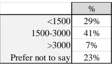
% <1500 29% 1500-3000 41% >3000 7% Prefer not to say 23% Table 2-Percentage of subjects in the sample of the experiment for each monthly family income interval
% <18 3% [18,30[ 56% [30,50[ 33% [50,70] 7% >70 1% Table 3-Percentage of subjects in the sample of the experiment for each age interval