Mapping the Pasture Steppe in Bayankhongor, Mongolia: comparison of classification methods, using Landsat-8 and geophysical data

(1)

i

Catarina Isabel Gouveia Lopes

Licenciada em Ciências e Engenharia do Ambiente

Mapping the Pasture Steppe in Bayankhongor, Mongolia:

comparison of classification methods, using Landsat-8

and geophysical data

Dissertação para obtenção do Grau de Mestre em

Engenharia do Ambiente, Perfil de Engenharia de Sistemas Ambientais

Orientador: Prof. Doutora Maria Júlia Seixas, Professora Auxiliar, FCT/UNL

Co-orientador: Doutor Nuno Santos Grosso, DEIMOS Engenharia SA

Presidente: Prof. Doutora Maria Teresa Calvão Rodrigues

Arguente: Doutor Nuno Miguel Matias Carvalhais

Vogal: Prof. Doutora Maria Júlia Fonseca de Seixas

Novembro de 2015

(2)

(3)

iii

Mapping the Pasture Steppe in Bayankhongor, Mongolia: comparison of classification methods, using Landsat-8 and geophysical data

A Faculdade de Ciências e Tecnologia e a Universidade Nova de Lisboa têm o direito, perpétuo e sem limites geográficos, de arquivar e publicar esta dissertação através de exemplares impressos reproduzidos em papel ou de forma digital, ou por qualquer outro meio conhecido ou que venha a ser inventado, e de a divulgar através de repositórios científicos e de admitir a sua cópia e distribuição com objectivos educacionais ou de investigação, não comerciais, desde que seja dado crédito ao autor e editor.

(4)

(5)

v

Acknowledgments

I would like to thank everyone who took part on the elaboration of this thesis, but also to everyone who participated in my academic journey in FCT/UNL.

First, I would like to thank my supervisors, Júlia Seixas and Nuno Grosso. To professor Júlia Seixas, by raising my interest for remote sensing, through her interesting lessons, and for providing the support necessary to finish this thesis; and to Nuno Grosso for having the patience for always guiding, advising and readily clarify any emergent questions throughout the whole development process of this thesis.

To DEIMOS Engenharia SA team who received me on the best possible way and provided me a place to work on my thesis. A special acknowledgement to Carla Patinha, who was always available for helping me whenever I needed to clarify any questions.

A huge thanks to my family, specially to my parents for all the dedication and effort that they have put on my education over the years. To my brother, for helping me on the reviewing process, but also for his support. To Eduardo who has been present for the major part of my academic years and always gave me the motivation and support to get through the most difficult times and helped me solve emerging problems of this thesis, by providing convenient suggestions.

I would also like to thank all of my university colleagues who accompanied me throughout this course. A special acknowledgment to the ones who were always present and to whom I owe all these great academic years: Carolina, Bruno and Diana.

(6)

(7)

vii

Abstract

Grasslands in semi-arid regions, like Mongolian steppes, are facing desertification and degradation processes, due to climate change. Mongolia’s main economic activity consists on an extensive livestock production and, therefore, it is a concerning matter for the decision makers. Remote sensing and Geographic Information Systems provide the tools for advanced ecosystem management and have been widely used for monitoring and management of pasture resources. This study investigates which is the higher thematic detail that is possible to achieve through remote sensing, to map the steppe vegetation, using medium resolution earth observation imagery in three districts (soums) of Mongolia: Dzag, Buutsagaan and Khureemaral. After considering different thematic levels of detail for classifying the steppe vegetation, the existent pasture types within the steppe were chosen to be mapped. In order to investigate which combination of data sets yields the best results and which classification algorithm is more suitable for incorporating these data sets, a comparison between different classification methods were tested for the study area. Sixteen classifications were performed using different combinations of estimators, Landsat-8 (spectral bands and Landsat-8 NDVI-derived) and geophysical data (elevation, mean annual precipitation and mean annual temperature) using two classification algorithms, maximum likelihood and decision tree. Results showed that the best performing model was the one that incorporated Landsat-8 bands with mean annual precipitation and mean annual temperature (Model 13), using the decision tree. For maximum likelihood, the model that incorporated Landsat-8 bands with mean annual precipitation (Model 5) and the one that incorporated Landsat-8 bands with mean annual precipitation and mean annual temperature (Model 13), achieved the higher accuracies for this algorithm. The decision tree models consistently outperformed the maximum likelihood ones.

Keywords: Remote sensing; Geographic Information Systems; Landsat-8; geophysical data; maximum likelihood; decision tree

(8)

(9)

ix

Resumo

As pastagens em regiões semi-áridas, como as estepes da Mongólia, estão actualmente a sofrer processos de desertificação e degradação devido às alterações climáticas. A maior actividade económica da Mongólia consiste na produção extensiva de gado, representando assim uma matéria de grande importância nos processos de tomada de decisão. A detecção remota e os Sistemas de Informação Geográfica providenciam ferramentas para a gestão avançada de ecossistemas e têm vindo a ser utilizados para monitorizar e gerir os recursos associados às pastagens. Este estudo investiga qual o nível mais elevado de detalhe temático que é possível alcançar para mapear a vegetação da estepe, através de detecção remota e do uso de imagens de observação da Terra de média resolução, em três distritos da Mongólia: Dzag, Buutsagaan e Khureemaral. Após terem sido considerados diferentes níveis de detalhe temático para classificar a vegetação da estepe, foi escolhido mapear os diferentes tipos de pastagens da estepe. De forma a investigar qual a combinação de dados que produz melhores resultados e qual o algoritmo de classificação mais apropriado para incorporar esses dados na classificação, foram testados e comparados diferentes métodos de classificação para a área de estudo. Para tal, foram realizadas dezasseis classificações utilizando diferentes combinações de estimadores, Landsat-8 (bandas espectrais e NDVI-derivado de Landsat-8) e dados geofísicos (altitude, precipitação média anual e temperatura média anual) com dois algoritmos de classificação, máxima verosimilhança e árvores de decisão. Os resultados revelam que o melhor modelo gerado para a árvore de decisão foi aquele que incorporava as bandas de Landsat-8 com a precipitação média anual e temperatura média anual (Modelo 13). Para a máxima verosimilhança, tanto o modelo que incorporava as bandas de Landsat-8 com a precipitação média anual (Modelo 5), como o que incorporava as bandas de Landsat-8 com a precipitação média anual e temperatura média anual (Modelo 13), obtiveram as acurácias mais elevadas para este algoritmo. Os modelos relativos à árvore de decisão obtiveram consistentemente melhores resultados do que aqueles que foram gerados pela máxima verosimilhança.

Palavras-chave: Detecção remota; Sistemas de Informação Geográfica; Landsat-8; dados geofísicos; máxima verosimilhança; árvore de decisão

(10)

(11)

xi

xiii

List of Figures

Figure 2.1 - Composition of a decision tree. Retrieved from Friedl and Brodley, 1997 ... 28

Figure 3.1 - Average summer temperature trend (1940-2005). Retrieved from Dagvadorj et al., 2009 ... 30

Figure 3.2 - Average winter temperature trend (1940-2005). Retrieved from Dagvadorj et al., 2009... 30

Figure 3.3 - Warm season precipitation trend (1940-2005). Retrieved from Dagvadorj et al., 2009 ... 30

Figure 3.4 - Study area: Dzag, Khureemaral and Buutsagaan soums located in Bayankhongor aimag, Mongolia ... 31

Figure 3.5 - Landsat-8 OLI false-color image using OLI-5, OLI-6 and OLI-2 mapped to RGB for Dzag, Khureemaral and Buutsagaan ... 32

Figure 3.6 – Landsat-8 NDVI-derived with 30 m resolution for the study area ... 33

Figure 3.7 - Elevation data from SRTM with 30 m resolution for the study area ... 34

Figure 3.8 - Mean annual precipitation data from 1950 to 2000 with 1 km resolution for the study area .... 35

Figure 3.9 - Mean annual temperature data from 1950 to 2000 with 1 km resolution for the study area .... 35

Figure 4.1 – TWI derived from SRTM data set for the study area ... 39

Figure 4.2 – Selected TWI to fit “water and riparian vegetation” ... 40

Figure 4.3 –Vector mask covering “water and riparian vegetation” classes ... 40

Figure 4.4 - Flow chart representing the output models for the main classes (M1, M2, M3 and M4), created using Landsat-8 bands from 1 to 7 (M1) and the same bands with NDVI (M2); and using 5, OLI-6 and OLI-7 (M3) and the same bands with NDVI (M4) ... 40

Figure 4.5 - Training points provided by the local users ... 42

Figure 4.6 - Testing points provided by the local users ... 42

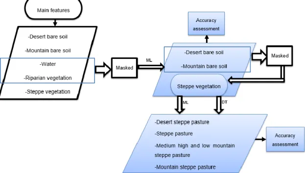
Figure 4.7 - Flow chart for output models created with different combinations of datasets used for classifying the Pasture Steppe classes: bands OLI-2 to OLI-7 with NDVI, SRTM, mean annual (MA) precipitation and mean annual (MA) temperature. The arrows represent the addition of a new estimator or a new model. Each model represents a classification output by using one estimator (base model – M1) or by the addition of one or more estimators to the base model ... 44

Figure 4.8 - Overview on the methods used to classify the main classes and the steppe vegetation (*ML-maximum likelihood classifier; DT- decision tree classifier) ... 47

Figure 5.1 - Spectral signatures for the main classes using Landsat-8 bands: OLI-1, OLI-2, OLI-3, OLI-4, OLI-5, OLI-6 and OLI-7 – Model 1 ... 49

Figure 5.2 - Spectral signatures for the main classes using Landsat-8 bands: OLI-1, OLI-2, OLI-3, OLI-4, OLI-5, OLI-6 and OLI-7 and NDVI [band 8] – Model 2 ... 49

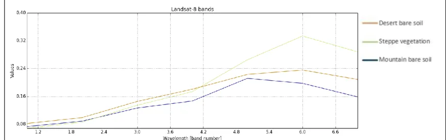
Figure 5.3 - Spectral signatures for the main classes using Landsat-8 bands: OLI-5, OLI-6 and OLI-7 – Model 3 ... 50

Figure 5.4 - Spectral signatures for the main classes using Landsat-8 bands: OLI-5, OLI-6 and OLI-7 and NDVI [band 8] – Model 4 ... 50

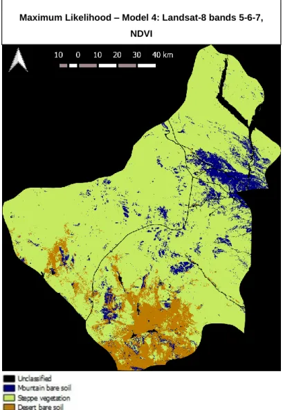
Figure 5.5 - Main classes using maximum likelihood - Model 4: Landsat-8 bands and NDVI ... 52

Figure 5.6 - Spectral signatures for the steppe vegetation classes using Landsat-8 bands: 2, 3, OLI-4, OLI-5, OLI-6 and OLI-7 – Model 1 ... 58

Figure 5.7 - Spectral signatures for the steppe vegetation classes using Landsat-8 bands: 2, 3, OLI-4, OLI-5, OLI-6 and OLI-7 and NDVI [band 8] – Model 2 ... 58

Figure 5.8 - Spectral signatures for the steppe vegetation classes using Landsat-8 bands: 2, 3, OLI-4, OLI-5, OLI-6 and OLI-7 and SRTM [band 8] – Model 3 ... 59

Figure 5.9 - Spectral signatures for the steppe vegetation classes using Landsat-8 bands: 2, 3, OLI-4, OLI-5, OLI-6 and OLI-7 and mean annual precipitation (MA precip.) [band 8] – Model 5 ... 59

Figure 5.10 - Spectral signatures for the steppe vegetation classes using Landsat-8 bands: OLI-2, OLI-3, OLI-4, OLI-5, OLI-6 and OLI-7 and mean annual temperature (MA temp.) [band 8] – Model 9 ... 60

(14)

xiv

Figure 5.11 - “Desert steppe pasture” F1-scores for all tested models using decision tree and maximum

likelihood ... 62

Figure 5.12 - “Steppe pasture” F1-scores for all tested models using decision tree and maximum likelihood ... 62

Figure 5.13 - “Medium high and low mountain steppe pasture” F1-scores for all tested models using decision tree and maximum likelihood ... 64

Figure 5.14 - “Mountain steppe pasture” F1-scores for all tested models using decision tree and maximum likelihood ... 65

Figure 5.15 - Steppe classification using maximum likelihood - Model 5: Landsat-8 bands, MA precipitation ... 69

Figure 5.16 - Steppe classification using decision tree - Model 5: Landsat-8 bands, MA precipitation ... 69

Figure 5.17 - Steppe classification using maximum likelihood - Model 13: Landsat-8 bands, MA precipitation and MA temperature ... 70

Figure 5.18 - Steppe classification using decision tree - Model 13: Landsat-8 bands, MA precipitation and MA temperature ... 70

Figure 5.19 - F1-scores weighted average for all tested models using decision tree and maximum likelihood ... 71

Figure A.1 - Main classes using maximum likelihood - Model 1: Landsat-8 bands ... 82

Figure A.2 - Main classes using maximum likelihood - Model 2: Landsat-8 bands and NDVI ... 82

Figure A.3 - Main classes using maximum likelihood - Model 4: Landsat-8 bands 5-6-7 and NDVI ... 83

Figure A.4 - Spectral signatures for the steppe vegetation classes using Landsat-8 bands: 2, 3, OLI-4, OLI-5, OLI-6 and OLI-7, NDVI [band 8] and SRTM [band 9] – Model 4 ... 84

Figure A.5 - Spectral signatures for the steppe vegetation classes using Landsat-8 bands: 2, 3, OLI-4, OLI-5, OLI-6 and OLI-7, NDVI [band 8] and mean annual precipitation (MA precip.) [band 9] – Model 6 ... 84

Figure A.6 - Spectral signatures for the steppe vegetation classes using Landsat-8 bands: 2, 3, OLI-4, OLI-5, OLI-6 and OLI-7, SRTM [band 8] and mean annual precipitation (MA precip.) [band 9] – Model 7 ... 85

Figure A.7 - Spectral signatures for the steppe vegetation classes using Landsat-8 bands: 2, 3, OLI-4, OLI-5, OLI-6 and OLI-7, NDVI [band 8], SRTM [band 9] and mean annual precipitation (MA precip.) [band 10] – Model 8 ... 85

Figure A.8 - Spectral signatures for the steppe vegetation classes using Landsat-8 bands: 2, 3, OLI-4, OLI-5, OLI-6 and OLI-7, NDVI [band 8] and mean annual temperature (MA temp.) [band 9] – Model 10 ... 86

Figure A.9 - Spectral signatures for the steppe vegetation classes using Landsat-8 bands: 2, 3, OLI-4, OLI-5, OLI-6 and OLI-7, SRTM [band 8] and mean annual temperature (MA temp.) [band 9] – Model 11 ... 86

Figure A.10 - Spectral signatures for the steppe vegetation classes using Landsat-8 bands: OLI-2, OLI-3, OLI-4, OLI-5, OLI-6 and OLI-7, NDVI [band 8], SRTM [band 9] and mean annual temperature (MA temp.) [band 10] – Model 12 ... 87

Figure A.11 - Spectral signatures for the steppe vegetation classes using Landsat-8 bands: OLI-2, OLI-3, OLI-4, OLI-5, OLI-6 and OLI-7, mean annual precipitation (MA precip.) [band 8] and mean annual temperature (MA temp.) [band 9] – Model 13 ... 87

Figure A.12 - Spectral signatures for the steppe vegetation classes using Landsat-8 bands: OLI-2, OLI-3, OLI-4, OLI-5, OLI-6 and OLI-7, NDVI [band 8], mean annual precipitation (MA precip.) [band 9] and mean annual temperature (MA temp.) [band 10] – Model 14 ... 88

Figure A.13 - Spectral signatures for the steppe vegetation classes using Landsat-8 bands: OLI-2, OLI-3, OLI-4, OLI-5, OLI-6 and OLI-7, SRTM [band 8], mean annual precipitation (MA precip.) [band 9] and mean annual temperature (MA temp.) [band 10] – Model 15 ... 88

Figure A.14 - Spectral signatures for the steppe vegetation classes using Landsat-8 bands: OLI-2, OLI-3, OLI-4, OLI-5, OLI-6 and OLI-7, NDVI [band 8] SRTM [band 9], mean annual precipitation (MA precip.) [band 10] and mean annual temperature (MA temp.) [band 11] – Model 16 ... 89

(15)

xv

Figure A.16 - Steppe classification using decision tree - Model 1: Landsat-8 bands ... 90

Figure A.17 - Steppe classification using maximum likelihood - Model 2: Landsat-8 bands and NDVI ... 91

Figure A.18 - Steppe classification using decision tree - Model 2: Landsat-8 bands and NDVI ... 91

Figure A.19 - Steppe classification using maximum likelihood - Model 3: Landsat-8 bands and SRTM ... 92

Figure A.20 - Steppe classification using decision tree - Model 3: Landsat-8 bands and SRTM ... 92

Figure A.21 - Steppe classification using maximum likelihood - Model 4: Landsat-8 bands, NDVI and SRTM ... 93

Figure A.22 - Steppe classification using decision tree - Model 4: Landsat-8 bands, NDVI and SRTM ... 93

Figure A.23 - Steppe classification using maximum likelihood - Model 6: Landsat-8 bands, MA precipitation and NDVI ... 94

Figure A.24 - Steppe classification using decision tree - Model 6: Landsat-8 bands, MA precipitation and NDVI ... 94

Figure A.25 - Steppe classification using maximum likelihood - Model 7 Landsat-8 bands, MA precipitation and SRTM ... 95

Figure A.26 - Steppe classification using decision tree - Model 7 Landsat-8 bands, MA precipitation and SRTM ... 95

Figure A.27 - Steppe classification using maximum likelihood - Model 8: Landsat-8 bands, MA precipitation, NDVI and SRTM ... 96

Figure A.28 - Steppe classification using decision tree - Model 8: Landsat-8 bands, MA precipitation, NDVI and SRTM ... 96

Figure A.29 - Steppe classification using maximum likelihood - Model 9: Landsat-8 bands, MA temperature ... 97

Figure A.30 - Steppe classification using decision tree - Model 9: Landsat-8 bands, MA temperature ... 97

Figure A.31 - Steppe classification using maximum likelihood - Model 10: Landsat-8 bands, MA temperature and NDVI ... 98

Figure A.32 - Steppe classification using decision tree - Model 10: Landsat-8 bands, MA temperature and NDVI ... 98

Figure A.33 - Steppe classification using maximum likelihood - Model 11: Landsat-8 bands, MA temperature and SRTM ... 99

Figure A.34 - Steppe classification using decision tree - Model 11: Landsat-8 bands, MA temperature and SRTM ... 99

Figure A.35 - Steppe classification using maximum likelihood - Model 12: Landsat-8 bands, MA temperature, NDVI and SRTM ... 100

Figure A.36 - Steppe classification using decision tree - Model 12: Landsat-8 bands, MA temperature, NDVI and SRTM ... 100

Figure A.37 - Steppe classification using maximum likelihood - Model 14: Landsat-8 bands, MA precipitation, MA temperature, NDVI ... 101

Figure A.38 - Steppe classification using decision tree - Model 14: Landsat-8 bands, MA precipitation, MA temperature, NDVI ... 101

Figure A.39 - Steppe classification using maximum likelihood - Model 15: Landsat-8 bands, MA precipitation, MA temperature, SRTM ... 102

Figure A.40 - Steppe classification using decision tree - Model 15: Landsat-8 bands, MA precipitation, MA temperature, SRTM ... 102

Figure A.41 - Steppe classification using maximum likelihood - Model 16: Landsat-8 bands, MA precipitation, MA temperature, NDVI, SRTM... 103

Figure A.42 - Steppe classification using decision tree - Model 16: Landsat-8 bands, MA precipitation, MA temperature, NDVI, SRTM ... 103

(16)

(17)

xvii

List of Tables

Table 3.1 - Landsat-8 OLI available bands for this work: description, wavelength and resolution. Adapted from Roy et al., 2014. ... 31 Table 4.1 - Weighting for each pasture class based on the real area extent per class used for calculate F1-scores weighted averages ... 46 Table 5.1 - Accuracy report for the main classes classification using maximum likelihood for Model 1, Model 2, Model 3 and Model 4 ... 51 Table 5.2 - Increasing (+) and decreasing (-) classification accuracies generated by the addition of Landsat-8 NDVI-derived: comparison of pairs of models with and without NDVI ... 54 Table 5.3 - Increasing (+) and decreasing (-) classification accuracies generated by the addition of SRTM data set: comparison of pairs of models with and without SRTM ... 55 Table 5.4 - Increasing (+) and decreasing (-) classification accuracies generated by the addition of mean annual precipitation data set: comparison of pairs of models with and without mean annual precipitation……... ... 56 Table 5.5 - Increasing (+) and decreasing (-) classification accuracies generated by the addiction of mean annual temperature data set: comparison of pairs of models with and without mean annual temperature ... 57 Table 5.6 - Accuracy report for the classification of the Pasture Steppe vegetation for the best F1-scores weighted average: Model 5 and Model 13 for maximum likelihood and Model 13 for decision tree (highlighted in blue) ... 63 Table 5.7 – Mapped areas per class and classified area in proportion to real area extent for the best performing models (highlighted in blue): Model 5 and Model 13 using maximum likelihood and decision tree ... 68 Table A.1 - Accuracy report of the Pasture Steppe using maximum likelihood and decision tree classifiers for Model 1, Model 2 and Model 3 ... 104 Table A.2 - Accuracy report of the Pasture Steppe using maximum likelihood and decision tree classifiers for Model 4, Model 6 and Model 7 ... 105 Table A.3 - Accuracy report of the Pasture Steppe using maximum likelihood and decision tree classifiers for Model 8, Model 9 and Model 10 ... 106 Table A.4 - Accuracy report of the Pasture Steppe using maximum likelihood and decision tree classifiers for Model 11, Model 12 and Model 14 ... 107 Table A.5 - Accuracy report of the Pasture Steppe using maximum likelihood and decision tree classifiers for Model 15 and Model 16 ... 108

(18)

(19)

xix

Acronyms

ASTER - Advanced Spaceborn Thermal Emission and Reflection Radiometer ADB - Asian Development Bank

AGB - Above Ground Biomass

AVHRR - Advanced Very High Resolution Radiometer AVIS-2 - Visible/Infrared Imaging Spectrometer DEM – Digital Elevation Model

DM - Drought Monitoring EO - Earth Observation

EOTAP - Earth Observation for a Changing Asia Pacific EVI - Enhanced Vegetation Index

GIS – Geographic Information System GPS - Global Positioning System

HRV - High Resolution Visible

JFPR - Japan Fund for Poverty Reduction LAI – Leaf Area Index

Landsat MSS – Landsat Multispectral Scanner Landsat TM – Landsat Thematic Mapper

Landsat-7 ETM+ - Landsat-7 Enhanced Thematic Mapper Plus Landsat-8 OLI – Landsat-8 Operational Land Imager

LULC – Land Use/ Land Cover

MODIS - Moderate-Resolution Imaging Spectroradiometer NDVI – Normalized Difference Vegetation Index

NIR – Near-infrared Qgis - Quantum GIS RGB - Red-Green-Blue RS – Remote sensing ROI – Region of Interest

SPOT - Satellite for Earth Observation. From French: Satellite Pour l’Observation de la Terre

SRTM - Shuttle Radar Topographic Mission TWI - Topographic Wetness Index

(20)

(21)

21 1. Introduction

1.1 Problem definition and previous approaches review

The vast grasslands of Mongolia are part of the steppe that is located between forest and desert belts of Inner Asia and Central Asia (Sutie et al., 2005). Steppe vegetation is determined by climatic and edaphic factors which promote grasses and associated herbaceous plants growth and prevent dominance of woody plants, such as trees and shrubs (Wallis de Vries et al., 1996). Mongolian steppes occur at a semi-arid climate and are among the largest contiguous expanses of grassland in the world, encompassing a region of considerable ecological importance (Badarch

et al., 2009).

Grasslands in Mongolia cover 1 210 000 km2_{(around 80 percent of the land area of the}

country) (Sutie et al., 2005) and support around 30 million head of domestic livestock, including camels, cattle, yaks, horses, sheep and goats and also populations of wild ungulates (Fernandez-Gimenez and Allen-Diaz, 2001). Mongolia has an extensive livestock production which constitutes the main economic activity in the country (Sutie et al., 2005).

Grasslands in arid and semi-arid regions are facing desertification or degradation processes caused by climate change and human activities (He et al., 2005), leading to negative impacts on herder livelihoods, carbon sequestration and biodiversity conservation (Jun Wang et

al., 2014). Since 1940 average temperature in Mongolia has increased by more than 2 ºC and

total precipitation dropped by 7% (16 mm), causing that Mongolia’s fragile steppe ecosystem to degrade at a rapid rate (Badarch et al., 2009). As a consequence of climate change, there has been an increased frequency of droughts occurrence in Mongolia, causing decreases in phytomass and changes in phenology (Shinoda et al., 2010). The occurrence of droughts during the early growth may cause vegetation to die before reaching maturity, shortening the growth period and decrease net primary production (Shinoda et al., 2007). Additionally, in the last 70 years, population density increased by more than threefold and total livestock numbers by more than 2,3-fold interfering with ecological balance and causing problems like overgrazing, which accelerated vegetation degradation (Karnieli et al., 2013).

The occurrence of land degradation in large areas is problematic because the resources (money, personnel and technology) available are limited (He et al., 2005). Monitoring and managing these processes within grasslands using field surveys for mapping vegetation might be difficult to accomplish, since these are expensive, manpower-demanding, time consuming (Karnieli et al., 2013) and may be incompatible with the increasing demand for precisely located spatial data of natural sites (Král and Pavlis, 2006). For this reason, satellite remote sensing has been widely used for a large number of vegetation applications (Karnieli et al., 2013).

Remote Sensing (RS) and Geographic Information System (GIS) provide the tools for advanced ecosystem management (Koirala, 2010). RS methods have been widely used for monitoring and management of pasture resources and GIS has become the most powerful tool

(22)

22

for providing information about grassland resource inventories and integration of data and mechanisms for analysis, modeling and forecasting. In order to offer the decision-makers the best tools and data to support their decision making process, it is important to define and classify accurately the land cover (Rodriguez, 2014). Satellite remote sensing data can provide data sources for large areas in land cover classification (Kawamura and Akiyama, 2010) . For mapping pasture resources, thematic information may be generated by applying image classification using parametric, non-parametric algorithms or a combination of both (Amarsaikhan and Sato, 2003).

However, there are many factors that can affect the success of a classification procedure, such as the complexity of the landscape in a study area, selected remotely sensed data, image pre-processing and classification approaches. For this reason, classifying remotely sensed data into a thematic map still remains a challenge. Although much research concerned with image classification has been done previously, the continuous emergence of new classification algorithms and techniques demand continuous reviews for guiding and selecting suitable classification procedures for specific studies (Lu and Weng, 2007).

The major problem tackled in this study, concerns the thematic level of detail for mapping vegetation, which is dependent on the imagery spatial resolution of the remotely sensed data. In order to provide information for livestock management resources, mapping vegetation species composition can provide the most detailed information for this purpose. However, since species composition varies within the different pasture types, influenced by geophysical factors, mapping these features can also provide important information. Additionally, mapping grassland properties could indicate which areas are more or less productive for livestock, helping on the definition of emergency grazing reserves (grazing areas in a good state for livestock production that can be used when droughts occur or when overgrazed areas are prominent).

1.2 Scope and objectives

This thesis was motivated and developed under the project “Climate-resilient rural livelihoods in Mongolia” that supports EOTAP (Earth Observation for a Changing Asia Pacific) and conducted at DEIMOS Engenharia SA company. The project aims to help the Mongolian Governmental Agencies to develop a sustainable, climate proof livestock sector, able to overcome the productivity and income loss problems, related to overgrazing and climate change, though Earth Observation (EO) services, that include a Land Use/ Land Cover (LULC) service and a Drought Monitoring (DM) service.

The current study is linked to the LULC mapping service that complements a previous Asian Development Bank (ADB) project funded by the Japan Fund for Poverty Reduction (JFPR), where some non-EO pasture type condition maps for Bayankhongor were already developed to help the local users to implement pasture management measures. The goal of this thesis is to map the steppe vegetation into relevant thematic classes, capable of providing information for the definition of areas to set aside as emergency grazing reserves by the local users, in three districts

(23)

23

(soums) - Dzag, Khureemaral and Buutsagaan – within Bayankhongor province (aimag), Mongolia.

The main objectives of this study are:

1. To find out the higher thematic detail to map the steppe vegetation through remote sensing data, to serve the purpose of defining emergency grazing reserves for the livestock.

2. To compare different combinations of Landsat-8 (spectral bands and Landsat-8 NDVI-derived) and geophysical data (including elevation, mean annual precipitation and mean annual temperature data), using two classification algorithms, in order to investigate which combination of data sets yields the best results and which classification algorithm is more suitable for incorporating these data sets when performing the classification.

1.3 Thesis structure overview

This thesis is divided into six chapters. Chapter 1 is an introductory chapter that presents the problem definition and previous approaches review, scope and objectives and the current thesis structure overview. Chapter 2 contains a literature review divided into three sections. The first provides information about the importance of imagery spatial resolution and field measurements, for mapping species composition and other pasture vegetation properties, that could be of importance for the definition of livestock emergency grazing areas. The second section focus on different procedures for mapping pasture types and the third section presents a review about classification algorithms.

Chapter 3 is also divided into three sections. The first gives a general overview about the study area. The second and third sections describe the collected data for performing the LULC classification. Chapter 4 presents the adopted methodology and the procedures to achieve the goal and objectives of this thesis. Chapter 5 describes the results and discussion obtained for the LULC classification, through a comparison analysis between the selected data sets and classification algorithms. Chapter 6 presents the main conclusions, summarizing the developed work, main results and limitations. At the end, recommendations for future research developments are given.

(24)

24 2.1 Mapping species composition and other grassland properties

through remote sensing data: the importance of spatial

resolution and field measurements

Spatial dimension of key land elements may range from less than one meter to more than one kilometer, depending on the potential of the optical satellite imagery used in the classification. A key land element is defined as a physical component of the land that characterizes one or more land cover classes. Therefore, the capacity to detect all of the key land elements is strongly correlated with the spatial resolution of the RS data. If the pixel spatial resolution is larger than the dimension of the land elements, it is not possible to detect the single land elements (Martinez and Mollicone, 2012) .

For instance, using a coarse resolution sensor (250-1000 m), such as NOAA-AVHRR (National Oceanic and Atmospheric Administration- Advanced Very High Resolution Radiometer), SPOT (satellite for EO. From French: Satellite Pour l’Observation de la Terre,) or Terra-MODIS (Moderate-Resolution Imaging Spectroradiometer), the potentially identifiable key land elements are only broad land cover patterns. Whereas if medium resolution sensor (30-60 m) is used, such as Landsat MSS (MultiSpectral Scanner), Landsat TM (Thematic Mapper), Landsat ETM+ (Enhanced Thematic Mapper Plus) or Landsat OLI (Operational Land Imager), separating extensive masses of evergreen and deciduous forest becomes possible. And by using high resolution sensors (10-30 m), such as Terra-ASTER (Advanced Spaceborn Thermal Emission and Reflection Radiometer) or SPOT-4 HRV (High Resolution Visible), or very high (<10 m) resolution sensors, such as SPOT-5, IKONOS or QuickBird, recognizing large individual trees becomes possible (Martinez and Mollicone, 2012).

Concerning the land use category grassland, the land elements are grasses and shrubs (Martinez and Mollicone, 2012). In fact, even for very high resolution it is difficult to achieve good results in discriminating species composition. For instance, Schmidtlein and Sassin (2004), used Airborne Visible/Infrared Imaging Spectrometer (AVIS-2) with a pixel size of 2 by 2 m, but the models obtained for the cover of single species proved to be weak. Reflectance of vegetation is very complex, because it depends on variables, like plant health, physical and chemical vegetation structure. For this reason, it is only partially correlated with plant species composition, making it the most difficult vegetation attribute to detect with remote sensing techniques (Lewis, 1998).

Apart from species composition, it is important to consider other grassland properties, because they can be used to define areas of major interest within the grasslands and may be important indicators for the classification procedure. Different grassland properties have been quantified from remotely sensed data, including grass cover and its temporal change, grassland biomass, yield and grassland degradation. Quantification of other grassland features, like productivity and carrying capacity, rely on environmental variables that cannot be acquired directly from remotely sensed data. These features require data that is difficult to obtain without field observations and ground sampling (e.g. soil fertility and moisture content) (Gao, 2006).

(25)

25

Zha et al. (2003) attempted to apply a reflectance-based method to quantify percent grass cover from Landsat TM data for a semi-arid grassland. Field measurements for the spectral reflectance of grass were made at 68 random sites and each location was determined with a portable Global Positioning System (GPS). Results showed that percent grass cover sampled on the ground does not verify a statistically significant relationship with the value of its corresponding pixel value on TM-derived Normalized Difference Vegetation Index (NDVI) image. The authors concluded that it was impossible to quantify percent grass cover using this sample point method directly. The main explanation for this, is that in situ grass cover measurement was made in a sampling plot of 1 m2_{, while NDVI pixel value is based on a ground area of 30 by 30 m}2_{, making}

very unlikely that the site at which ground cover was sampled is representative at the entire pixel area. Also, NDVI values derived from satellite image range from 0,4067 to 0,5805, much narrower than from in situ measurements, ranging within 0,2898 to 0,6283. However, satisfactory results were obtained when the spectral reflectance data measured with the field spectrometer was used to calibrate satellite data (R2_{= 0,74).}

Liu et al. (2005) used a similar methodology to study grassland cover density in an alpine meadow soil. Similar results were obtained showing that in situ sampled grass cover and their corresponding pixel values on the NDVI image were weakly correlated. After calibrating satellite data with the spectral reflectance data, a strong linear regression relationship (R2_{= 0,745) was}

established. These results reveal the need for combining remotely sensed data with in situ sampling and locating ground samples on geometrically rectified satellite images.

Karnieli et al. (2013) studied the reliability of remote sensing vegetation indices to provide information about the effect of grazing on vegetation degradation. This research was taken along the Mongolian pastures in six study sites, three of them located within the mountain steppe zone and the other three at the steppe zone. Each site consisted in pairs of study polygons comprising an ungrazed (fenced-off) area and a heavily grazed area (outside the fences). The selected vegetation index was the Enhanced Vegetation Index (EVI), in order to reduce the soil background and atmospheric effects throughout the entire study area and also because it is more sensitive to variations in leaf cellular structure, expressed in the near infrared (NIR) portion of the spectrum. Four Landsat-7 ETM+ images were used to create a continuous scene and EVI was computed from reflectance values. Ground truth data was collected to provide information about biophysical variables (plant density, species composition, above ground biomass (AGB), and percentage cover) and plant spectral reflectance. Field observations showed that plant density, AGB and percentage cover values were significantly higher in the ungrazed areas than in the grazed ones, as expected. However, the grazed areas showed significantly higher EVI values than the ungrazed areas, consistently in each of the study sites. This result was found to be linked with the presence of unpalatable species that invaded into the grazed areas, which promoted the shifting of dominant species composition from “climax” species, like perennial grasses and forbs, to unpalatable forbs and weedy annuals, which have a denser leaf structure and therefore inducing higher spectral responses in near-infrared (NIR) region.

(26)

26

Imagery spatial resolution also plays an important role in obtaining a reliable quantification of grassland properties. For instance, spatial resolutions suitable for estimating Leaf Area Index (LAI) lie between 2 and 18 m (being the most accurate at 2 and 5 m). Also, the ratio of NIR and visible reflectance is considered a poor predictor of LAI or biomass (Sellers, 1985). (Phinn et al., 1996) used high spatial resolution Airborne Digital Video Imagery to map AGB for five major semi-arid plant communities in New Mexico. Results show that beyond 2 to 4 m pixel size, shrub forms became unrecognizable. Variations in NDVI values due to spatial differences in vegetation cover, biomass and/or vigor conditions were evident at larger pixel sizes, however NDVI patterns become undistinguishable for detecting biomass from 4,6 m pixel size in the more continuously covered grassland. Up to 8 m pixel sizes features larger than individual shrubs were evident, including bare and vegetated areas and soil.

2.2 Mapping pasture types: satellite data, vegetation indices and

geophysical factors

The use of high resolution remotely sensed data presents some disadvantages associated with infrequent coverage, high costs and high data volume. Consequently, coarse and medium resolution satellites have been used by researchers for producing regional scale land cover classifications (Wang and Tenhunen, 2004). Monitoring land cover requires spectral coverage and resolution that is well suited for vegetation characterization. For this tasks, spectral coverage in the visible, near infrared and shortwave infrared are required (Wulder et al., 2008). Landsat data provides medium resolution data with no costs for the users. Throughout more than 40 years, Landsat mission has demonstrated capabilities for mapping and monitoring land cover and its value is well established (Roy et al., 2014).

A vegetation index consists on a simple and effective measurement used to access earth’s surface vegetation in remote sensing. There are several indices for highlighting vegetation features (Gandhi et al., 2015). The Normalized Difference Vegetation Index (NDVI) is one of the most commonly used remote sensing derived measurement (Yu et al., 2003). It is calculated as a ratio difference between red and near-infrared (NIR) bands, either from the digital number or reflectance values (Liu et al., 2003). NDVI data can be combined with satellite data for improving classification’s accuracy, for instance, Gandhi et al. (2015) used Landsat TM data along with satellite NDVI-derived and elevation data, to perform a land cover classification of Vellore District. Sivanpillai et al., 2009 verified that the predictive ability for the estimation of sagebrush cover categories using vegetation indices, including NDVI, was 1% higher than the predictive ability of Landsat TM spectral bands over a semi-arid ecosystem in Western US.

Pasture types distribution are strongly influenced by geographic features and their impacts on climate (Yu et al., 2003) being mainly affected by elevation, temperature and precipitation (Wen et al., 2010). Several studies show improvements when remotely sensed data is combined with geophysical data. For instance, Liu et al., 2003 stacked three geophysical data sets (elevation, mean annual precipitation and mean annual temperature) together with Advanced

(27)

27

Very High Resolution Radiometer (AVHRR) and AVHRR NDVI-derived data after dividing China into nine bio-climatic regions. The nine land-cover maps for individual regions of China were then assembled. Results showed that the combination of remotely sensed data with geophysical data sets can improve the classification of spatial patterns of vegetation distribution and contribute for the reduction of confusion in the land cover classification.

Liu et al. (1998) verified an improvement on land cover classification of Northeast China, when geophysical data (precipitation, temperature and elevation) was added to an AVHRR image, compared to a conventional classification method using only AVHRR data. Cibula and Nyquist (1987) verified that an increase on the number of land cover classes that could be differentiated using terrain, temperature and precipitation resulted on an improvement of classification’s accuracy. Liu et al. (1998) combined a model that described the relationships between land cover, slope and elevation, that resulted on an accuracy improvement for the vegetation classification using Landsat TM spectral data on Helan Mountain in China (Liu et al., 2003).

2.3 Classification algorithms

GIS plays an important role in developing knowledge-based classification approaches because of its capability of managing different sources of data and spatial modelling. As different types of ancillary data, such as: Digital Elevation Model (DEM), soil map, precipitation and temperature, become available they can be incorporated into the classification procedure. This leads to the possibility of separating vegetation classes using data on terrain features or using temperature, precipitation and soil data to predict land cover distribution at a large scale. Including these relationships in a classification procedure has proven to be effective in improving classification accuracy. A critical step is to develop approaches to identify the best appropriate variables that are most useful in separating land cover classes. The success of an image classification depends mostly on the availability of high-quality remotely sensed imagery and ancillary data, the design of a proper classification procedure, and the analyst’s skills and experiences (Lu and Weng, 2007 ).

Per-pixel classifiers typically develop a signature through the combination of the spectra of all training-set pixels from a given feature. This signature contains the contributions of all the materials present in training pixels. It does not take into account the impact of mixed pixels. Per pixel classification algorithms can be parametric or non-parametric, such as maximum likelihood, minimum distance, artificial neural network, decision tree and support vector machine (Lu and Weng, 2007).

The maximum likelihood classifier is widely used for mapping land cover features. It is based on the assumption that the members of each class follow a Gaussian frequency distribution, that evaluates the membership probability of an unknown pixel to be assigned to a given class. Each pixel is assigned to a class for which it has the highest membership probability

(28)

28

value. This classifier involves the estimation of class mean vectors and covariance matrices from the training data (Pal and Mather, 2003).

When multisource data is used in a classification procedure, parametric algorithms, such as maximum likelihood, are typically not appropriated. Non-parametric classifiers are especially suitable for the incorporation of non-remote-sensing data into the classification procedure, because no statistical parameters are needed to separate image classes (Lu and Weng, 2007). One of the most commonly used non-parametric classifiers is the decision tree classifier. The decision tree uses a multi-stage or sequential approach to the problem. Unlike conventional statistical classifiers, the labeling process is based on simple decisions based on the results of sequential tests, rather than a simple complex decision (Pal and Mather, 2003).

The decision tree classification procedure consists on a recursively partition of a data set into smaller homogeneous subdivisions on the basis of tests defined at each node in the tree, applied to one or more feature values. Figure 2.1, defines the composition of a tree, where each box is a node at which tests (T) are applied to recursively split data into successively smaller groups. The labels (A, B, C) at each leaf node refer to the class label assigned to each observation (Friedl and Brodley, 1997).

Figure 2.1 - Composition of a decision tree. Retrieved from Friedl and Brodley, 1997

There are univariate and multivariate decision trees. The univariate decision tree is one in which the decision boundaries of each node are defined by the outcome of a test applied to a single feature evaluated at each node. The characteristics of the decision boundaries are estimated empirically from the training data. The test outcome splits the data into two or more subsets. Each test has a discrete number of outcomes. The input data is recursively partitioned until a leaf node is reached and the class label is assigned to the observation. For cases when the locations of decision boundaries in feature space can only be properly defined in terms of combinations of features, the univariate tree is not appropriated (Pal and Mather, 2003).

The multivariate decision tree is a more complex tree, than the univariate which introduces factors that can affect their performance. It allows the extension of the splits to include

(29)

29

linear combinations of features. A set of linear discriminant functions is estimated at each node of the multivariate tree. Also, any number of different algorithms can be used to estimate the splitting rule. When different classification algorithms are used at different nodes it is called a hybrid decision tree (Pal and Mather, 2003).

3. Study area and data

3.1 General characterization of the study area

Mongolia is located in central Asia, being bounded on the north by Russia and on the east, south and west by China. It has a total area of 1 565 000 km2_{. The topography of Mongolia}

consists mainly of a vast plateau with an elevation that ranges from 914 to 1524 m, with mountain ranges in the north and west reaching to heights of 4267 m above sea level (Dagvadorj et al., 2009).

There are six vegetation zones in Mongolia based on different elevation, precipitation distribution and soil type: alpine tundra (3,0% of the area), mountain taiga (4,1%), mountain steppe (25,1%), steppe (26,1%), desert steppe (27,2%) and desert (14,5%). Biological yield of Mongolian pastures can range from 1050-1500 kg/ha in high mountain, to 650-1300 kg/ha in steppe and to 290-380 kg/ha in desert steppe. Vegetation growing season is short and very dependent on climate, particularly rainfall. New growth in the northern mountainous areas begins in mid-April, but on other regions it may not begin until mid-May. Some of the pasture species reach their final growth stage in August, but others may continue its vegetative growth until mid-September or remain green until October (Damiran, 2005).

The climate is cold semi-arid and markedly continental (Sutie et al., 2005) characterized by short hot summers, in which falls most of the annual precipitation (85-90% in June, July and August) (Dagvadorg et al., 2001) and long cold winters. Winter and spring are both typically windy and cold. In early summer and spring frequently occur severe droughts and strong winds (with velocities exceeding 20 m/s) (Sutie et al., 2005), that may cause low productivity of vegetation in this area. Increases in spring temperature may stimulate earlier vegetation photosynthesis activity and, at the same time, increase the water stress in arid and semi-arid ecosystems (Dagvadorg et

al., 2001).

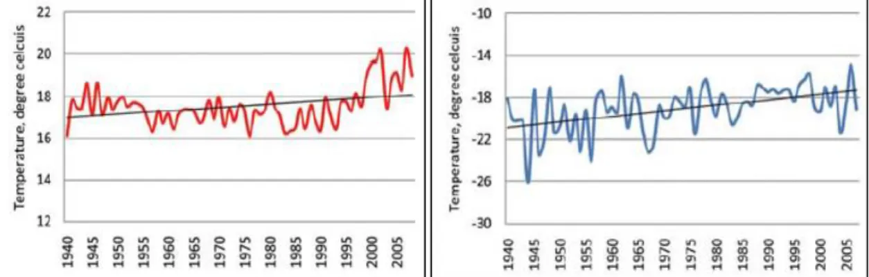
Figures 3.1 and 3.2 show the increase registered on average temperature in summer and winter seasons, respectively. Figure 3.3 presents the 16 mm decrease on average precipitation registered in Mongolia, from 1940 to 2005 (Dagvadorj et al., 2009). In Bayankhongor, summer temperatures increased significantly from 1984 to 2003 in mountain steppe, steppe and desert steppe, spring temperatures also increased (Khishigbayar et al., 2015).

(30)

30

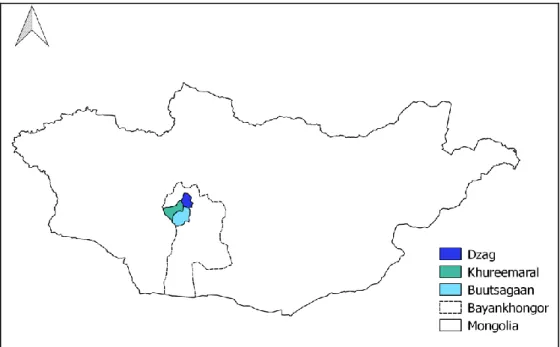
The study area consists of three soums: Dzag (46°56'N, 99°9’E), Khureemaral (46°24'N, 98°17'E) and Buutsagaan (46°10'N, 98°41'E) located in Bayankhongor aimag, Mongolia (Figure 3.4). Dzag has a total land area of 432800 ha; Khureemaral, 584000 ha; and Buutsagaan, 256100 ha. A document provided by the local users shows the existing pasture types within the steppe and also the main vegetation species composition.

Figure 3.3 - Warm season precipitation trend (1940-2005). Retrieved from Dagvadorj et al., 2009

Dzag has 88 km2 _{of high mountain pasture, mainly dominated by Festuca lenensis. The}

mountain steppe pasture covers an area of approximately 1426 km2 _{, having Festuca lenensis,} Stipa krilovii and Artemisa frigida as the dominant species. The steppe pasture covers an area of

779 km2_{and it is mainly composed by Leymus chinensis, Festuca lenensis and Stipa orientalis.}

Interzonal river valleys and depressions meadow pasture occupies an area of 237 km2_{, being}

mainly composed by Artemisa frigida.

Khureemaral has 1571 km2_{of medium high and low mountain steppe pasture with} Festuca lenensis, Artemisa frigida and Stipa krilovii. The steppe pasture covers an area of 1990

km2_{, being mainly composed by Stipa krilovii, Stipa capilata, Artemisa frigida, Agropyron} cristatum, Leymus chinensis and Festuca lenensis. The desert steppe pasture occupies 611 km2

and it is mainly dominated by Stipa gobica and Artemisa frigida. It also contains interzonal river valleys and depressions meadow pasture, with Achnatherum slendens, Allium polyrrhizum and

Kalidium gracile, covering an area of 159 km2_.

Figure 3.2 - Average winter temperature trend (1940-2005). Retrieved from Dagvadorj et al., 2009 Figure 3.1 - Average summer temperature

trend (1940-2005). Retrieved from Dagvadorj et al., 2009

(31)

31

Buutsagaan has 2362 km2_{occupied by medium high and low mountain steppe pasture,}

mainly composed by Festuca lenensis, Stipa gobica, Caragana pygmaea and Artemisa frigida. The steppe pasture covers 1051 km2_{with Festuca lenensis, Stipa krilovii and Caragana pygmaea.}

The desert steppe pasture covers 1712 km2_{, being mainly composed by Stipa gobica, Anabasis} brevifolia, Allium polyrrhizum, Caragana pygmaea, Cleistogenes squarrosa, Artemisa xerophytica

and Ajiana fruticosa. The gobi desert pasture occupies 30 km2_{and it is composed by Anabasis} brevifolia and Allium polyrrihizum. Interzonal river valleys and depressions meadow pasture

occupies 166 km2_{within the soum and it is mainly composed by Allium polyrrhizum, Kalidium} gracile and Achnatherum splendens.

3.2 Remotely sensed data

The imagery used for the classification consists of Landsat-8 OLI seven bands with 30 m resolution, retrieved from earthexplorer.usgs.gov. The image is from 30 August 2014, corresponding to the summer season. The Landsat-8 imagery contains the spectral information of seven bands, as listed in Table 3.1.

Table 3.1 - Landsat-8 OLI available bands for this work: description, wavelength and resolution. Adapted from Roy et al., 2014.

Band description Wavelength (µm) Resolution (m)

OLI-1 – blue 0,43 – 0,45 30

OLI-2 - blue 0,45 – 0,51 30

Figure 3.4 - Study area: Dzag, Khureemaral and Buutsagaan soums located in Bayankhongor aimag, Mongolia

(32)

32

OLI-3 – green 0,53 – 0,59 30

OLI-4 – red 0,64 – 0,67 30

OLI-5 – near infrared 0,85 – 0,88 30

OLI-6 – shortwave infrared 1,57 – 1,65 30

OLI-7 – shortwave infrared 2,11 – 2,29 30

The Landsat-8 false-color image using OLI-5, OLI-6 and OLI-2 mapped to Red-Green-Blue (RGB), is presented in Figure 3.5. In this false-color composite, healthy vegetation appears in shades of orange; green represents sparse grasslands; soils appear in shades of browns and purples; and clear deep water is very dark. Google Earth was used to visually confirm these assumptions.

NDVI ratio was calculated using red and NIR bands (OLI-4 and OLI-5, respectively), accordingly to Equation 3.1.

𝑁𝐷𝑉𝐼 =

𝑁𝐼𝑅−𝑅𝐸𝐷_{𝑁𝐼𝑅+𝑅𝐸𝐷} Equation 3.1

Landsat-8 false-color composite

Figure 3.5 - Landsat-8 OLI false-color image using OLI-5, OLI-6 and OLI-2 mapped to RGB for Dzag, Khureemaral and Buutsagaan

(33)

33

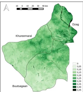
NDVI values range from -1,0 to 1,0 (Weiss et al., 2004), variating with the absorption of red light by plant chlorophyll and the reflection of infrared radiation by water-filled leaf cells. In other words, the degree of greenness is equal to vegetation’s chlorophyll concentration (Gandhi

et al., 2015). The positive values (NIR>RED) indicate green vegetated surfaces, and as the NDVI

values increase, the vegetation greenness increases with it. Negative values indicate non-vegetated areas, such as water, ice, snow and bare soil (Weiss et al., 2004). Landsat-8 NDVI-derived is presented in Figure 3.6.

Figure 3.6 – Landsat-8 NDVI-derived with 30 m resolution for the study area

3.3 Geophysical data

3.3.1 Elevation data

The Shuttle Radar Topographic Mission (SRTM) Void Filled data set with 30 m resolution was retrieved from earthexplorer.usgs.gov. It contains elevation data that results from additional processing to address areas of missing data or voids. These voids were filled using interpolation algorithms in conjunction with other sources of elevation data.

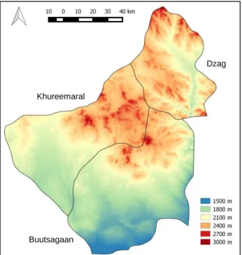
Figure 3.7 shows the elevation data from SRTM, used to complement the spectral information from Landsat-8 bands. The elevation at the study area ranges from 1433 m to 3005 m. In Dzag elevation ranges from 1826 m to 3005 m, being the soum that reaches the highest elevation. Mountain steppe pasture is expected to be found on the higher elevations of this soum, along with steppe pasture, on lower regions. Buutsagaan’s elevation ranges from 1432 m to 2919 m, reaching the lower elevation of the three soums; Khureemaral’s elevation ranges from 1737 m to 2871.The desert steppe pasture is expected to be on the lower elevations of Buutsagaan

Dzag

Khureemaral

(34)

34

and Khureemaral and on the higher elevations of this two soums, medium high and low mountain steppe pasture and steppe pasture are expected to be.

Figure 3.7 - Elevation data from SRTM with 30 m resolution for the study area

3.3.2 Precipitation and temperature data

Mean annual precipitation and mean annual temperature data sets were extracted from worldclim.org, both being for the time period between 1950 to 2000. Despite the time period not including the years between 2000 to 2014, annual climatic means would not change drastically within fourteen years, in order to change the spatial distribution of the Pasture Steppe vegetation.

The resolution of the precipitation and temperature data is 30 seconds (approximately 1 km). Since finding a better resolution for precipitation and temperature data was not possible, these two layers will be taken as a lower resolution than the Landsat-8 and SRTM images.

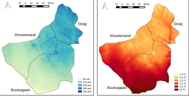
Mean annual precipitation and mean annual temperature images are represented in figures 3.8 and 3.9, respectively. In Dzag mean annual precipitation ranges from 146 mm to 237 mm and mean annual temperature ranges from -7,5 ºC to -2,3 ºC, reaching the higher mean annual precipitation and the lower temperature values from the three soums. Mountain steppe pasture is expected to be found where higher values of mean annual precipitation and lower values of mean annual temperature are present. For lower precipitation values and higher temperature values is where the steppe pasture is expected to be found.

In Buutsagaan, mean annual precipitation ranges from 81 mm to 201 mm and mean annual temperature ranges from -6,5 ºC to 0,8 ºC, reaching the lower mean annual precipitation and the higher mean annual temperature of the study area. In Khureemaral, mean annual precipitation ranges from 93 mm to 184 mm and mean annual temperature ranges from -6,6 ºC to -0,8 ºC. In Khureemaral and Buutsagaan, where the lower mean annual precipitation values and the higher mean annual temperature values are, is where the desert steppe pasture is

Buutsagaan Khureemaral

(35)

35

expected to be located. Whereas, higher mean annual precipitation and lower mean annual temperature values are correspondent to medium high and low mountain steppe pasture and steppe pasture.

3.4 Data pre-processing

Python functions created, in collaboration with DEIMOS team, were applied to perform cloud, water and snow masks to the spectral bands of Landsat-8 and two mosaics comprising the study area were joined on the SRTM data set. Mean annual precipitation and mean annual temperature data sets were subjected to a re-projection from 1 km to 30 m resolution, in order to be used along Landsat-8 and SRTM data. This task was performed on Qgis.

Since multisource estimators (Landsat-8 and geophysical data) were combined on the classification procedure, a standardization of the data was needed. All the estimators (Landsat-8, NDVI, SRTM, mean annual precipitation and mean annual temperature) were converted to z-scores, which is a dimensionless quantity that sets the data values to a zero mean (Helldén and Tottrup, 2008). The z-score is calculated by determining the mean and standard deviation for each estimator and then subtracting the mean from each estimator, finally it divides this value by its standard deviation. It is given by Equation 3.2, where 𝑥 is a raw score to be standardized, 𝜎 is the standard deviation of the population and 𝜇 is the mean of the population (Helldén and Tottrup, 2008). The estimators standardization was performed using a Python function created in collaboration with DEIMOS team.

𝑧 =

𝑥 − 𝜇

𝜎 Equation 3.2

Figure 3.9 - Mean annual temperature data from 1950 to 2000 with 1 km resolution for the study area

Figure 3.8 - Mean annual precipitation data from 1950 to 2000 with 1 km resolution for the study area Buutsagaan Dzag Khureemaral Khureemaral Dzag Buutsagaan

(36)

(37)

37 4. Methods

4.1 Selection of a suitable classification method

Since the images available for this study are from Landsat-8 with a spatial resolution of 30 m, discriminating the different species and other vegetation features will not be possible, because the dimension of the land elements (grasses and shrubs) is much smaller than the spatial resolution of the images. Additionally, since collecting field information at the study site was not possible, quantifying grassland properties, like AGB and yield, plant density, productivity, LAI, or percentage cover was considered to be infeasible. It is possible that these properties, relying only on vegetation indices, could provide misleading information, to the local users, for the definition of emergency grazing reserves, because of the possible presence of unpalatable plants that might have invaded the grazed areas. For the stated reasons, discriminating the steppe into its different pasture types was considered to be the best option for achieving the goal of this thesis.

The nomenclature used for the pasture types follows the same of the training points provided by the local users. The training points provided by the local users were collected on field campaigns, by a team of the Ministry of Industry and Agriculture (Project Management Unit – PMU) in collaboration with JFPR. Based on the training points provided, the study area has been classified into: “desert steppe pasture”, “steppe pasture”, “medium high and low mountain steppe pasture” and “mountain steppe pasture”. One point for “gobi desert steppe pasture” and another for “interzonal river valleys and depressions meadow pasture” were also provided, but they were excluded, because it would be necessary more points to map these classes.

On the first attempts to classify the study area into the four aimed classes, the results showed low accuracies, because there was a high confusion among “medium high and low mountain steppe pasture” and “mountain steppe pasture” and also “medium high and low mountain steppe pasture” with “steppe pasture”. The confusion among different land cover classes can be reduced through masking areas that are not to be classified, but have similar spectral properties, providing the capability for achieving a greater control over the classification process (McCloy, 1995). (Xian et al., 2015) wanted to map shrubland components across the northwest United States, but a confusion between other land cover classes existed. In order to perform a hierarchical classification approach, a mask of non-shrubland areas, such as forests, urban and agriculture was created.

In this case, classifying and then masking the non-steppe land cover classes, present at the study area, was considered to be the best approach for performing a more accurate classification of the pasture steppe classes. For this reason, the main classes present at the study area were identified, in order to reduce the classification confusion among the Pasture Steppe classes. The next section, 4.1.1, explains in more detail the procedure for the identification and classification of the main classes and section 4.1.2 describes the classification of the steppe vegetation into its different pasture types, after masking the main classes.

(38)

38 4.1.1 Main classes – Bare soil, water and vegetation

Using the Landsat-8 image, with seven spectral bands with false color composition on RGB of OLI-5, OLI-6 and OLI-2 (Figure 3.5) and Google Earth software, five main classes were identified: two classes for bare soil: “desert bare soil” and “mountain bare soil”; one class for rivers and waterbodies “water”; and two classes for vegetation “riparian vegetation” and “steppe vegetation”. Mountain bare soil is mainly seen in Dzag in shades of purples, but also in Khureemaral and Buutsagaan in shades of browns. Desert bare soil appears in shades of gray in Khureemaral and Buutsagaan. Rivers are very dark and waterbodies are black and purple. The riparian vegetation represents the interface between terrestrial and aquatic ecosystems, it appears in shades of orange alongside the rivers and waterbodies of the study area. Because of its proximity to water, the riparian vegetation is much more luxuriant than the sparse vegetation present at the steppe vegetation (shades of greens). NDVI confirms it, because its values are considerably higher alongside rivers and waterbodies (Figure 3.6). Even though this main class consists on vegetation it was chosen to mask it, because the riparian vegetation is not allocated to any of the pasture classes selected for the classification.

Since no training nor testing points, collected in the field, were available, the Regions of Interest (ROI) were defined, based on Landsat-8 image (Figure 3.5) and Google Earth satellite images, in order to perform a supervised classification. These ROIs were created with the semi-automatic classification plugin on Quantum GIS (Qgis). For the collection of the training and testing data preference was given to pixels that were located in homogeneous areas with neighboring pixels belonging to the same class.

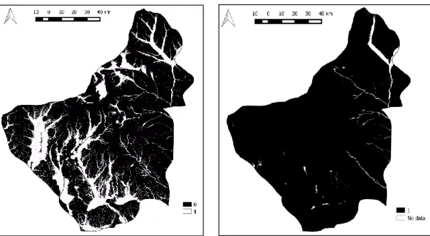
The classification was performed using the seven bands: 1, 2, 3, 4, OLI-5, OLI-6 and OLI-7. These bands were also combined with Landsat-8 NDVI-derived to try a better separation of the vegetation classes from soil and water classes. Since non-remotely-sensed data would not be incorporated into this classification procedure, the maximum likelihood classifier was used. When the main classes classification was performed using maximum likelihood, a high confusion among “mountain bare soil” and “water” classes was detected. To reduce this confusion, a classification using only three bands: OLI-5, OLI-6 and OLI-7 was also performed, because in these wavelengths the spectral signatures were better separated, than for the remaining wavelengths. However, since the confusion among “mountain bare soil” and “water” classes still remained, the “water” class was masked, so that the classification of the remaining classes could be performed. To mask the “water” class the Topographic Wetness Index (TWI) derived from the SRTM data set was performed on Qgis.

TWI is a DEM-based index that works as a proxy for soil moisture, functioning as a relative measure of the long-term soil moisture availability of a given site. TWI is defined by Equation 4.1, where As is the specific catchment area (the cumulative upslope area draining through a cell divided by the contour width), and β is the local slope (Kopecký and Cizková, 2010).

𝑇𝑊𝐼 = 𝑙𝑛

𝐴𝑠