SIMULATION OF THE VELOCITY FIELD IN COMPOUND CHANNEL FLOW USING
DIFFERENT CLOSURE MODELS
M. Filonovich
1,3, R. Azevedo
1, L. R. Rojas-Solorzano
2and J. B. Leal
1,31
Universidade Nova de Lisboa, Faculdade de Ciências e Tecnologia, Caparica, Portugal
2
Universidad Simón Bolívar, Caracas, Venezuela
3
CEHIDRO, Instituto Superior Técnico, Lisbon, Portugal
ABSTRACT
In this study a comparison of three turbulence closure models (two isotropic and one anisotropic) with experimental data is performed. The interaction between the main channel (MC) flow and the floodplain (FP) generates a complex flow structure. A shallow mixing layer develops between the MC flow and the slower FP flow generating a high horizontal shear layer, streamwise and vertical vortices, momentum transfer and other phenomena, related to velocity retardation and acceleration. This phenomenon dissipates part of the kinetic energy and contributes to the reduction of the velocity differences between the MC and the FP. The large scale vortices that are generated in the shear layer are anisotropic, provoking the formation of secondary flow cells that influence the primary velocity distribution. These three-dimensional turbulent structures can be reasonable well reproduced by a simple anisotropic model (Algebraic Stress Model). The isotropic models are capable of simulating the boundary layer, especially the model base in -ω equations, but cannot simulate the shear layer that develops at the interface.
INTRODUCTION
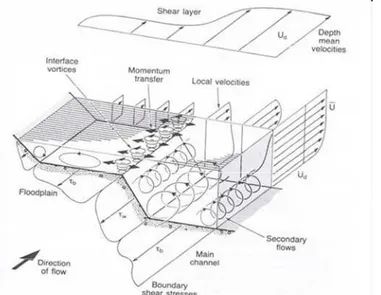
Most natural rivers have compound cross-section composed by a main channel and by one or more floodplains on the lateral sides. For most of the time the water flows only in the main channel, however, when flooding occurs the water depth exceeds the bank full depth of the main channel and thus overflow occurs on the floodplains. The fast flow in the main channel is retarded by the slower flow on the floodplains, causing lateral momentum transfer. The shear layer that develops at the interface of the main channel and the floodplain by the difference of velocities affects turbulence structures and streamwise and vertical vortices are developed. Turbulent structures in compound channel flow indicate three-dimensional (3D) behavior (Fig. 1). There are two kinds of vortices that are generated at the interface between the main channel and the floodplain; one is a horizontal vortex due to shear layer of the streamwise flow, first observed by Sellin (1964), and the other is the secondary flow in the cross section due to anisotropy of turbulence, also called secondary flow of 2nd kind ( . Nezu and Nakagawa, 1993). These effects have been observed experimentally by Shiono and Knight (1991), and Tominaga and Nezu (1991) using fiber-optic Laser-Doppler anemometer (LDA) and numerically by Naot . (1993), using an algebraic Reynolds stress model (ARSM), by Shiono and Lin (1992) and Pezzinga (1994), using a non-linear -ε model and by Cokljat and Younis (1995), using the full Reynolds-stress transport model. They have found a significant influence of secondary flows onto momentum transfer and boundary shear stress.
Figure 1. Three dimensional description of compound channel flow by Shiono and Knight (1991).
is used, then secondary flows are accurately simulated and the distribution of mean primary velocity and the wall shear stress are also accurately reproduced. But the main difficulty lies in the choice of the turbulence model. Thus, isotropic eddy viscosity models, like the standard k-ε model, are robust and economic but are incapable of producing secondary flows. Instead, the ARSM is being often used lately; it reasonably predicts secondary flows and is computationally economic compared to Direct Numerical Simulation, DNS, or more complex models ( . . Large Eddy Simulation, LES).
The present study simulates the uniform flow in compound channel for high relative depth (≈ 50%), using ANSYS CFX Computational Fluid Dynamics (CFD) code. For this purpose -ε model, Shear Stress Transport (SST) model and Explicit Algebraic Reynolds Stress Model (EARSM) were employed. The -ε model and SST model are isotropic models based on Boussinesq’s approximation and do not produce secondary flows, while EARSM is derived from the Reynolds stress transport equations and is able to simulate secondary flows caused by turbulence anisotropy . The main purpose of the study is comparison of the numerical results obtained by isotropic and anisotropic models with the experimental velocity results obtained by a Laser Doppler Velocimeter (LDV).
EXPERIMENTAL SET-UP AND EXPERIMENTS DETAILS
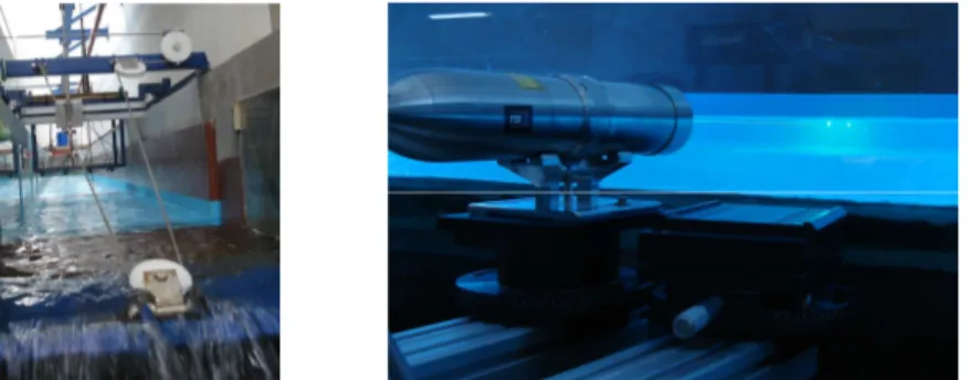
The experimental studies were carried out in the Hydraulics Laboratory of the University of Beira Interior in prismatic channel (Fig. 2a) with a bed slope = 0.001, 10 m length and with asymmetric trapezoidal compound section. The compound channel geometry and dimensions are shown in Figure 3. In this figure is the water level above channel bottom, is the bankfull level above channel bottom, main channel bottom width, and section width. The uniform regime was established by imposing a discharge of 24.7 l/s which corresponds to a relative height = ( – )/ ≈ 50%. The streamwise instantaneous velocity of the flow was measured using a LDV. Positioning of the system probe was achieved with 0.1 mm precision positioning system controlled by computer. The measurements were performed in back-scattering mode through the lateral glass of the channel (Fig. 2b). The water depth was measured using a point gauge and acoustic probes; the total discharge was measured using an electromagnetic flow meter installed in the recirculation pipe of the channel.
Figure 2. a) Photo with donstream view of the channel; b) Photo of the LDV measuring laterally.
º
Figure 3. Cross- section of the compound channel
!
"
"
!
#$!
% &'
#$!
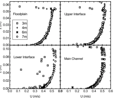
Figure 4. Measured vertical profiles of time-averaged velocity in the floodplain, in the upper and lower interfaces (Fig. 3), and in the middle of the main channel, at cross-sections = 3, 4, 6 and 7 m.
NUMERICAL MODELLING
The flow field was calculated using a commercial 3D CFD code (ANSYS CFX 12.0). This code uses a control-volume-based finite element method, where the governing equations are discretized over each control volume, using a second-order upwind scheme for the advection terms in momentum and turbulence equations. The resulting system is then solved in a coupled manner, and the results are then interpolated to the grid nodes. The convergence criterion was settled when a global mass imbalance was less than 0.1%.
In this work, the flow dynamics is modeled by numerically solving the Reynolds Averaged Navier-Stokes (RANS) equations for the water-air combination. To model the air-water segregated flow, the mass conservation of each phase is solved, while the momentum equation (RANS) for each phase is added up to eliminate the interphase momentum transfer term. There is a closure equation for the volume fraction, which states that both phases volume fraction must add up to one at every fluid cell. The free surface model is accompanied by an interphase sharpening algorithm, which guarantees a minimum diffusion of the volume fraction around the interphase.
The domain, exactly coincident with the experimental flume, was discretized using approximately 1,200,000 regular hexahedral elements aligned to the main directions. For turbulence modeling purposes, the + of the element closest to the bottom walls were kept around 20 for the floodplain and 50 for the main channel, using therefore, wall functions for all the turbulent models here explored.
A uniform velocity field with a water depth of 0.103m and 5% of turbulence intensity was prescribed at the inlet; while a hydrostatic pressure profile with zero velocity derivatives was set at the outlet. The upper boundary condition was prescribed on the air, at 0.05 m above the expected free surface, with free-slip wall to allow the free motion of the air along the channel, while facilitating the numerical robustness of the simulation. The bottom wall was prescribed with a non-slip boundary condition and an absolute roughness of 0.0002m.
Three different turbulence models were used; all based on the basic RANS equations: -ε model; Shear Stress (SST) model; and Explicit Algebraic Reynolds Stress Model (EARSM). The first two models belong to the family of isotropic two-equation models, while the third model captures the natural anisotropy within the wall turbulence and therefore, solves for the 6 Reynolds stresses. The standard -ε model with wall functions for dampening the turbulent viscosity near the walls is used (Rodi, 1993). The SST model accounts for the transport of the turbulent shear stress and uses a
combination of the best features of the -ε model for free turbulence, and the standard Wilcox -ω model for the solution of the wall turbulence (Menter, 1994). The use of this model in this study aims to determine the possible highly accurate predictions of the onset and the amount of flow separation under adverse pressure gradients. The EARSM represents an extension of the standard -ε two-equation model. This is derived from the Reynolds stress transport equations and gives a nonlinear relation between the Reynolds stresses and the mean strain-rate and vorticity tensors (Wallin and Johansson, 2000). This model is used in the present study due to the higher order terms it solves, such that it may be able to capture effects of secondary flows.
Vertical Profiles of Time-Averaged Velocity
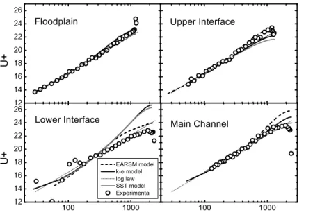
The vertical profiles of time-averaged velocity measured and simulated numerically with -ε, SST and EARSM turbulence models in cross-section = 7 m are presented in Fig. 5. The figure also includes the log-law ( . . Nezu and Nakagawa, 1993):
( )
1 ln
+ +
= +
κ (1)
where *
+
= is the non-dimensional flow velocity, is the shear velocity, κ is the von Kármán constant equal to
0.41, *
+
= νis the non-dimensional vertical coordinate,
ν
is the kinematic viscosity equal to 1,01x10⁻⁶ m2/s at 20ºC, and is a constant that for smooth bottoms takes the value 5.3 ( . Nezu and Nakagawa, 1993). The values of * and can be obtained by applying Clauser’s method ( . . Nezu and Nakagawa, 1993) where a linear regression is used to fit the data of ln( ) and inside the inner layer ( . ., / < 20%). A practically constant value of * = 0.022 m/s was obtained, while values of were more scattered ranging from 3 to 7.(
)*+,% -.
/ ,,0 )1
"
(
(
% &'
(
"
Figure 5. Measured and simulated ( -ε, SST and EARSM models) vertical profiles of time averaged velocity in the floodplain, in the upper and lower interfaces, and in the middle of the main channel, at cross-section = 7 m.
Analyzing the results presented in Fig. 5 one can conclude that, in the inner layer ( + < ≈450), all models give similar results and with good agreement with experimental data. Another conclusion is that in the floodplain and in the middle of the main channel the results seem almost independent of the turbulence model used and show good agreement with the experimental data, except near the free-surface. In the interface verticals and for the outer layer ( + > ≈450) EARSM model gives results slightly overestimated but closer to the experimental data than the other isotropic models. This means that the depth-averaged velocity in the floodplain can be computed using simplified models (isotropic), but in the upper and lower interfaces those models will, respectively, underestimate and overestimate the depth-averaged velocity, being necessary the use of anisotropic models like EARSM.
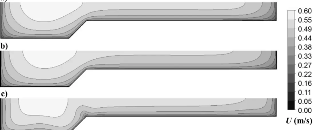
Isovel lines, secondary flow vectors, and TKE
The isovel lines obtained numerically with -ε, SST and EARSM turbulence models in cross-section = 7 m are presented in Fig. 7. The isovel lines of EARSM (Fig. 7c) bulge significantly upward near the upper interface as a result of secondary flow cells generated by turbulence anisotropy and represented in Fig. 1 ( . Nezu, 1994). The isovel lines of
-ε and SST don’t show that behavior since they assume isotropic turbulence and therefore cannot reproduce the secondary flow.
Figure 7. Isovel lines obtained numerically in cross-section = 7 m with turbulence model: a) -ε; b) SST; and c) EARSM.
Figure 8. Secondary flow vectors obtained numerically in cross-section = 7 m with EARSM turbulence model.
Figure 9. Turbulent Kinetic Energy (TKE) results [m2/s2], obtained numerically in cross-section = 7 m with turbulence model: a) -ε; b) SST; and c) EARSM.
Fig. 9 presents the Turbulent Kinetic Energy (TKE) results obtained numerically with -ε, SST and EARSM turbulence models in cross-section = 7 m. Comparing the results obtained with -ε model (Fig. 9a) and SST model (Fig. 9b), one can conclude that the latter performs better near the walls. This is because in CFX -ε is not optimized for boundary
a)
b)
c)
(m/s)
Maximum secondary vel. = 0.014 m/s
≈ 2.5% of primary vel.
a)
b)
layer flows, whereas SST model uses -ω equations near the walls which allow obtaining better results ( . Menter, 1994). Nevertheless, the EARSM shows the more realistic results (Fig. 9c), since it not only models the turbulence created by the walls, but it also simulates the turbulence arising from the interaction between the flows in the main channel and in the floodplain.
CONCLUSIONS
The numerical simulation of experimental results with three different turbulence models: -ε and SST, both isotropic, and EARSM, anisotropic, allowed to verify that using anisotropic turbulence models is required if velocity profiles are to be accurately predicted in the interface region. Isotropic models underestimate velocities in the upper interface and overestimate them in the lower interface. In the main channel isotropic models perform better and in the floodplain all models give similar results. Isovel lines, secondary flow vectors, and TKE numerical results confirm the relevance of modeling anisotropy in the sense that it generates secondary flow responsible for changing the isovel lines of streamwise velocity, especially in the upper interface where a shear layer develops.
ACKNOWLEDGMENTS
The authors wish to acknowledge the financial support of the Portuguese Foundation for Science and Technology through the project PTDC/ECM/70652/2006. The first and second authors wish to acknowledge the financial support of the Portuguese Foundation for Science and Technology through the Grants No. SFRH/BD/64337/2009 and
SFRH/BD/33646/2009, respectively.
REFERENCES
1. Bousmar, D.; Riviere, N.; Proust, S.; Paquier, A.; Morel, R. and Zech, Y. (2005) Upstream discharge distribution in
compound-channel flumes, , 131(5): 408-412.
2. Chow, V.T. (1959) , McGraw Hill, New York.
3. Cokljat, D. and Younis, B. (1995) Second Order Closure Study of Open-channel Flows, , 121(2): 94-107.
4. Lin, B. and Shiono, K. (1995) Numerical Modelling of Solute Transport in Compound Channel Flows, , 33(6): 773-788.
5. Menter, F.R. (1994) Two-equation eddy-viscosity turbulence models for engineering applications, , 32(8): 1598-1605.
6. Naot, D., Nezu, I. and Nakagawa, H. (1993) Calculation of compound open channel flow. , 119(12): 1418-1426.
7. Nezu, I. (1994) Compound open-channel turbulence and its role in river environment, ! "
# $ % , Keynote address, Singapore.
8. Nezu, I. and Nakagawa, H. (1993) & ' (, IAHR Monograph Series, A.A. Balkema, Rotterdam, Netherlands.
9. Pezzinga, G. (1994) Velocity distribution in compound channel flows by numerical modeling. , 120(10): 1176-1197.
10. Rodi, W. (1993) Turbulence Models and their Application in Hydraulics, a State of the Art Review, IAHR Monograph Series, 3rd edition, Delft.
11. Sellin, R.H.J. (1964) A laboratory investigation into the interaction between the flow in the channel of a river and that over its floodplain, ) , 7: 793-802.
12. Shiono, K. and Knight, D.W. (1991) Turbulent open-channel flows with variable depth across the channel,
* + , 222: 617-646.
13. Shiono, K. and Lin, B. (1992) Three Dimensional Numerical Models for Two Stage Open Channel Flows,
, -!./ " " , + + , ,
Ed. Gayer, Starosolszky, Maksimovic, pp. 123–130.
14. Sofialidis, D. and Prinos, P. (1998) Compound open-channel flow modeling with nonlinear low-reynolds k-ε models, , 124(3): 253-262.
15. Tominaga, A. and Nezu, I. (1991) Turbulent structure in compound open channel flows. , 117(1): 21-40.
16. Wallin, S. and Johansson, A. (2000) A complete explicit algebraic Reynolds stress model for incompressible and
compressible flows, * + ,403: 89-132.