Marina Filonovich
Faculdade de Ciências e Tecnologia Universidade Nova de Lisboa
NUMERICAL MODELLING OF
COMPOUND CHANNEL FLOW
Dissertação para obtenção do Grau de Doutor em Engenharia Civil
Orientador: João Gouveia Aparic
io Bento Leal
Assistant Professor, FCT/UNL,Portugal
Professor, Universitetet i Adger, Norway
Co-orientador: Luis R. Rojas-
Solórzano
Associate Professor
Nazarbayev University, Kazakhstan
Juri:
Presidente: Prof. Fernando Manuel Anjos Henriques
Arguentes: Prof. Rui Miguel Lage Ferreira
Prof. José Manuel Paixão Conde
Vogais: Prof. Mário Jorge Rodrigues Pereira de Franca
Prof. Maria Rita Lacerda Morgado
Fernandes de Carvalho Mesquita David
N
0de
Arquivo_______________________________
[Numerical Modelling of Compound Channel Flow]
Copyright © [Marina Filonovich], Faculdade de Ciências e Tecnologia, Universidade Nova de
Lisboa.
A Faculdade de Ciências e Tecnologia e a Universidade Nova de Lisboa têm o direito, perpétuo e sem limites geográficos, de arquivar e publicar esta dissertação através de exemplares
impressos reproduzidos em papel ou de forma digital, ou por qualquer outro meio conhecido ou
i
Acknowledgements
I would like to thank both the Civil Engineering Department of the Faculty of Sciences and Technology of New University of Lisbon (FCT/UNL) and the Foundation of Science and Technology (FCT) for providing the necessary resources and financial support through the scholarship SFRH/BD/64337/2009 and through the projects PTDC/ECM/70652/2006, PTDC/ECM/117660/2010 and RECI/ECM-HID/0371/2012 for the duration of this PhD.
There are numerous people that I would like to thank, both academically and socially, for enriching my life over the last four years.
First of all, I would like to express gratitude to my supervisors, Prof. João Gouveia Aparicio Bento Leal and Prof. Luis R. Rojas-Solórzano, for their guidance, enthusiasm and criticism, which allowed all of this to be possible. To both of them, for their great support and encouragement, for sharing with me your wealth of knowledge, for helpful discussions in person and remotely, I give my sincere and heartfelt thanks.
Prof. Rui Ferreira and Prof. Mário Franca deserve a special mention for organising the
International Workshops. Thank you for introducing me and having the opportunity to discuss and to have a feedback on my research work from the experts in fluvial hydraulics community and CFD modelling (Koji Shiono, Vladimir Nikora, Thorsten Stoesser, Wim Uijttewaal, Dubravka Pokrajac, to mention a few). Special gratitude to the experts for willing to share with us their invaluable experience. I am also grateful to George Constantinescu and Weiming Wu for their invaluable feedback on my research that took place at Master Class of the River Flow 2012 Congress in Costa Rica; and special thanks to Rafael Murillo, the organiser of the Congress, for making possible for me to attend this Master class.
Special thanks to our Travelling Nerds group (Stephan Spiller, Inés Mera Rico, Helena
Nogueira, Ana Margarida Ricardo, Bruño Fraga, Sándor Baranya and Mona Jafarnejad) for
spending unforgettable time in Costa Rica. It was a fantastic trip despite the earthquake, heavy rains and tropical virus. This was an adventure that will be remembered forever! Thank you for sharing with me this part of your lives, your Tovarisch!
I would like to express special thanks to my friends Matthew Wilkinson and his lovely wife Elizabete for enriching my social life and my English. Thank you for delightful dinners, barbecues and lots of parties. Matthew, your mushroom risotto and baked goat cheese will be always my favourite dish.
My thanks to Ian Paterson and Katarzyna Wojtyczka for inviting me and my family for the Christmas party, where we had a chance to know and become friends with these amazing and joyful people, Przemek Jankowski, Aleksandra Kawalek and Kenny Walker. Thanks to all of you for the wonderful time that we spent together during these several months. It is not much but it seems like we know each other forever and is so easy and comfortable to chat with you that time just flies (like during the Easter). Special thanks to Kenny for sharing with me the typical Portuguese recipe that most Portuguese people do not know. It was the best Arroz de Pato ever!
My thanks to João Fernandes, Hugo Biscaia and Noel Franco at this difficult final stage for
your help, support and understanding. I would also like to thank Ricardo Azevedo for providing me with the experimental data for validating my numerical simulations. To Moises Brito, Silvia
Saggiori, Sílvia Rute Amaral, Ricardo Birjukov Canelas, Olga Birjukova Canelas, Edgar
Ferreira, Rui Aleixo, Pawel Jerzy Wojcik, Iwona Bernacka-Wojcik many thanks for your help, support and just for sharing with me your experience and friendship.
ii
particularly, I’m grateful to Prof. Manuel A. J. Gonçalves de Silva, Prof. João C. G. Rocha de Almeida, Prof. Fernando M. A. Henriques, Prof. Válter J. G. Lúcio, Prof. António M. Pinho
Ramos and all others who not been specifically mentioned here. Special thanks to Carla Teixeira and to Maria da Luz Sousa for being not only good professionals but also good persons willing always to help and to listen.
The last months were not easy for me…being far away from my beloved husband and
daughter and finishing the PhD thesis, but I could always count on my friends Andrey Lyubchik
and his gorgeous wife Elena Lygina. I’m very grateful to them for helping me with my daily
problems in this difficult period of my life, for supporting and understanding.
I would also like to express my deep gratitude to my parents in-law for their encouragement and believing in me. Undoubtely, the completion of this research would not have been possible without their support.
At last but not least I would like to thank my husband Sergej for his love and care, patience, responsibility and understanding. Thank you for being tolerant when I was in a bad mood. You
are the best husband and I’m so lucky to have you! Ятебялюблю!
iii
Abstract
The main objectives of the present study are to evaluate the performance of most common RANS turbulence closure models in simulating river flows, where secondary currents play an important role, and to contribute to the understanding of the relative importance of the underlying physical hypotheses enclosed in each model. Guidelines for CFD users are also proposed, regarding mesh independence and computational domain approach.
For that purpose, ANSYS-CFX package was used allowing the simulation of uniform flows in straight asymmetric trapezoidal and rectangular compound channels with several different RANS turbulence closure models. Namely, isotropic k- and shear stress transport (SST) models and anisotropic explicit algebraic Reynolds stress models (EARSM) and Reynolds stress models (RSM). In anisotropic models two approaches were used for the near-wall region, one was the standard k- model and the other a modified k- model (BSL). Also different pressure-strain rate models were used: LRR-IP, LRR-IQ and SSG.
Verification and validation of the numerical solutions was performed using Grid Convergence Index method together with linear regression analysis. Local mesh refinement of regions of interest improved significantly the convergence of the turbulent field. The comparison of the simulations with existing experimental data showed better agreement for anisotropic models. Nevertheless, some discrepancies were observed and further analysed. The transport terms revealed to be important, which invalidates the hypothesis of negligible anisotropy diffusion implicit in the weak equilibrium condition of EARSM. The anisotropy convection and streamline curvature corrections, established for flow in rotating frames, did not improve the EARSM results. The RSM performs better than EARSM, but still presents problems due to limitations of the near-wall and free-surface modelling, of the adopted transport/diffusion and pressure-strain rate models, and to the isotropic dissipation rate assumption. The two former seem to have a higher impact on the quality of the solution.
v
Resumo
Os objectivos deste estudo foram a avaliação da performance de modelos de turbulência
(acoplados às equações RANS) na simulação de escoamentos fluviais com correntes
secundárias e contribuir para o conhecimento sobre a validade das hipóteses simplificativas de
cada modelo. Propuseram-se ainda procedimentos para utilizadores de CFD relativos à
independência da malha e à implementação do domínio de cálculo.
Foi utilizada a aplicação ANSYS-CFX na simulação de escoamentos uniformes em canais
rectos com secção composta assimétrica (rectangular e trapezoidal). Usaram-se modelos de
turbulência isotrópicos, k- e shear stress transport (SST), e anisotrópicos, explicit algebraic Reynolds stress models (EARSM) e Reynolds stress models (RSM). Nestes últimos testaram-se
duas abordagens para a região da parede, uma baseada no modelo k- e a outra num modelo k-
modificado (BSL). Testaram-se ainda diferentes modelos para a correlação da pressão com a
taxa de deformacão: LRR-IP, LRR-IQ e SSG.
A verificação e validação das soluções numéricas foi efectuada usando o método Grid Convergence Index juntamente com análise de regressão linear. O refinamento local da malha
nas regiões de interesse melhorou significativamente a convergência do campo turbulento. A comparação das simulações com dados experimentais existentes mostrou melhores resultados para os modelos anisotrópicos. Nestes, os termos de transporte revelaram-se importantes,
invalidando a hipótese de difusão anisotrópica desprezável, implicita no EARSM. As correcçöes da convecção da anisotropia e da curvatura das linhas de corrente, estabelecidas para
escoamentos com rotacão, não melhoraram a qualidade dos resultados do EARSM. O RSM
apresenta melhores resultados, mas ainda assim subsistem problemas relacionados com o
tratamento das regiões da parede e da superfície livre, com os modelos dos termos de transporte e de correlação da pressão com a taxa de deformação e com a hipótese de taxa de dissipação turbulenta isotrópica. Os dois primeiros parecem ter maior impacto na qualidade da solução.
Palavras-chave: canal de secção composta, leito principal, leito de cheia, modelo de
vii
Contents
1 Introduction……… 5
1.1 Background and motivation….…………...………. 5
1.2 Objectives and methodology..……….. 8
1.3 Thesis outline...………. 9
1.4 References………. 11
2 Basic concepts in turbulence modelling... 17
2.1 Introduction………... 17
2.2 Governing equations and Reynolds averaging... 17
2.3 Problems and limitations in turbulence modelling... 19
2.4 Eddy viscosity models... 20
2.5 Reynolds stress models... 26
2.5.1 Reynolds stress model... 26
2.5.2 Omega-based Reynolds stress models……...……….. 32
2.5.3 Algebraic Reynolds stress models... 33
2.5.4 Explicit algebraic Reynolds stress models... 34
2.6 References………. 39
3 Modelling approach...……… 47
3.1 Introduction to computational fluid dynamics (CFD)….………. 47
3.2 Structure of the ANSYS CFX...…..………. 48
3.3 Discretisation and solution theory.………... 51
3.3.1 Finite volume method (FVM)...……… 51
3.3.2 Numerical differentiation schemes……….. 54
3.3.3 Pressure-velocity coupling... 56
3.3.4 Linear equation solution and multigrid technique... 58
3.3.5 Boundary conditions and near-wall modelling... 59
3.3.6 Errors and uncertainty in CFD modelling... 64
3.4 References ………...…. 68
4 Literature review...………...……… 75
4.1 Introduction...……….. 75
4.2 Inbank flows in straight channels………...…..………. 77
4.2.1 Rectangular open-channels...…….……… 77
viii
4.3 Flow in straight compound channels.………... 86
4.3.1 Rectangular compound channels...……….. 88
4.3.2 Trapezoidal compound channels………...….. 94
4.4 References……….….………... 97
5 Summary of results... 105
5.1 Research Paper I: Credibility analysis of computational fluid dynamic simulations for compound channel flow... 105 5.2 Research Paper II: Simulation of the velocity field in compound channel flow using different closure models... 107 5.3 Research Paper III: Prediction of compound channel secondary flows using anisotropic turbulence models... 109 5.4 Research Paper IV: Open-channel secondary flow simulation with RSM and EARSM... 110 6 Conclusions and future research... 119
6.1 Conclusions……….. 119
6.2 Future research...………..………..……. 120
Appendix A Research Papers
ix
List of Figures
Figure 3.1. Structured and unstructured grids. 50
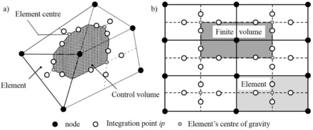
Figure 3.2. Control volume around grid node in 2D mesh: (a) unstructured; (b) structured.
52
Figure 3.3. Mesh element. 52
Figure 3.4. Coarsening for 3D grid. 59
Figure 3.5. Wall boundary conditions: (a) single fluid domain; (b) two-fluid domain.
61
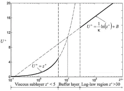
Figure 3.6. Subdivisions of the near-wall region. 63
Figure 4.1. Schematic representation of natural river. 76
Figure 4.2. Measured secondary-current velocity vectors at a section in: (a) closed duct; (b) open-channel (after Nezu 2005).
78
Figure 4.3. Isovels of streamwise velocity and secondary currents in rectangular open-channel for aspect ratio 2 (adapted from Tominaga
etal. 1989).
79
Figure 4.4. Calculated secondary current streamlines in open-channels under various aspect ratios (after Naot and Rodi 1982).
79
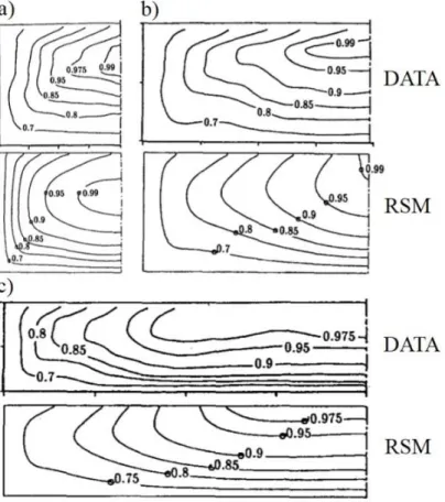
Figure 4.5. Predicted (RSM) and measured seconary flow in rectangular open-channel: Aspect ratios (a) 2; (b) 3.94; (c) 8 (adapted from Cokljat and Younis 1995).
80
Figure 4.6. Contours of primary velocity in rectangular open-channel: Aspect ratios (a) 2; (b) 3.94; (c) 8 (adapted from Cokljat and Younis 1995).
81
Figure 4.7. Predicted (RSM) and measured turbulence anisotropy for open rectangular channel with aspect ratio = 2 (adapted from Cokljat and Younis 1995).
82
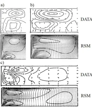
Figure 4.8. Secondary current vectors: (a) RSM by Kang and Choi (2006a); (b) experiment Nezu and Rodi (1985); (c) RSM by Cokljat (1993); and (d) LES by Shi etal. (1999) (adapted from Kang and Choi 2006a).
83
Figure 4.9. Secondary current vectors in smooth trapezoidal channels (adapted fromTominaga etal. 1989).
84
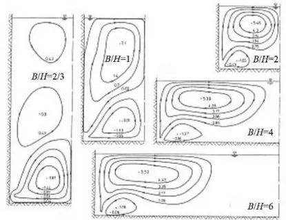
Figure 4.10. Secondary flow cells pattern in smooth trapezoidal channels with different aspect ratio: (a) 2b/H ≤ 2.2; (b) 2b/H ≥ 4 (adapted
fromKnight etal. 2007).
85
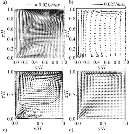
Figure 4.11. Velocity contours and secondary velocity vectors in smooth trapezoidal channels: (a) k-; (b) SSG; (c) SMC- (adapted from
x Knight etal. 2005).
Figure 4.12. Schematic representation of compound channel: (a) symmetric rectangular compound channel; (b) asymmetric rectangular compound channel; (c) symmetric trapezoidal compound channel and (d) asymmetric trapezoidal compound channel.
86
Figure 4.13. Hydraulic parameters associated with overbank flow in a trapezoidal compound channel (after Shiono and Knight 1991).
87
Figure 4.14. Schematic representation of flow field in: (a) a shallow depth flow; (b) deep depth flow (adapted from Nezu etal. 1999).
89
Figure 4.15. Experimental and computed contours of the streamwise velocity: (a) data by Tominaga et al. (1989); (b) model by Pezzinga (1994); (c) data by Tominaga and Nezu (1991) and (d) model by Sofialidis and Prinos (1998) (adapted from Pezzinga (1994) and Sofialidis and Prinos (1998)).
90
Figure 4.16. Vector plots of the secondary currents and contours of the primary velocity in asymmetric compound channels for hr = 0.5 (adapted
from Cokljat and Younis 1995).
91
Figure 4.17. Contours of the streamwise velocity in asymmetric compound channels for hr = 0.5 (adapted from Thomas and Williams 1995a,
Cater and Williams 2008, Kara etal. 2012).
93
Figure 4.18. Boundary shear stress in symmetric compound channel with trapezoidal cross-section (after Knight et al. 2005).
xi
List of Tables
Table 1.1. Top 10 important flood disasters for the period 1900 to 2014. 5 Table 1.2. The most devastating flood disasters. Top 10 at economic losses for
the period 1900 to 2014. 6
Table 2.1. Values of the constants in the k- model for open-channel flows
(Nezu and Nakagawa 1993). 23
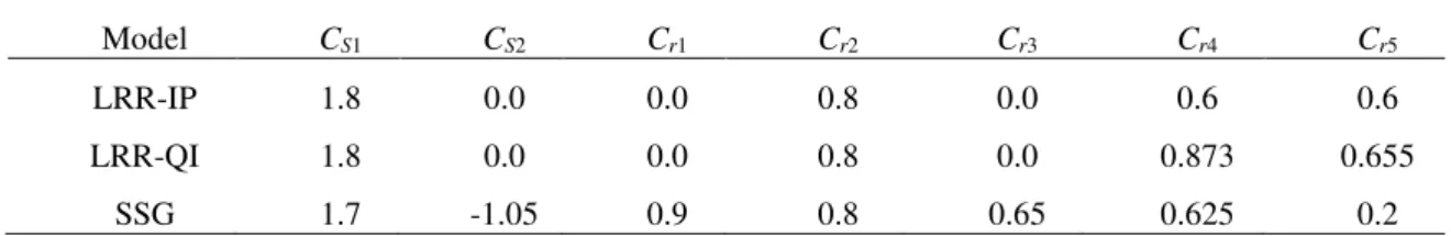
Table 2.2. Values of the constants in the the k- model (Wilcox 1988). 24 Table 2.3. Values of the coefficients in the BSL k- model. 25 Table 2.4. Values of the constants in the LRR-IP, LRR-QI and SSG models. 32
xiii
List of Abbreviations and Symbols
Latin alphabet
Symbol Description Units
A Cross sectional area; coefficient matrix [m 2]; [-]
A3 Coefficient from EARSM [-]
aij Reynolds stress anisotropy tensor [-]
B Total channel top width; constant in the logarithmic velocity law
[m]; [-]
Bfp Floodplain width [m]
Bmc Main channel top width [m]
b Main channel half bottom width in symmetric compound
channels; main channel bottom width in asymmetric compound channels
[m]; [m]
C Volume fraction [-]
CD Model constant [-]
CDiff Constant from EARSM [-]
C1, C2, C, Empirical constants in the k-ε model [-]
CS Coefficient from the gradient-diffusion model [-]
C1, C2 Rotta constant and constant from LRR-IP and LRR-QI
models
[-]
C1 Constant from EARSM [-]
CS1, CS2, Cr1, Cr2,
Cr3, Cr4, Cr5
Constants in the LLR-IP, LLR-QI and SSG models [-]
21
a e , 32
a
e Approximate relative error between meshes 1 and 2, and between meshes 2 and 3, respectively
[-]
Fs Factor of safety [-]
F1 Blending function [-]
f Darcy-Weisbach friction factor [-]
f1, f2, f3 Fine-, medium- and coarse grid solution of the variable of
interest obtained with grid spacing h1, h2 and h3,
respectively
[]
xiv
H Water depth [m]
hb Main channel bankfull height [m]
hfp Floodplain water depth [m]
h1, h2, h3, grid size of fine-, medium- and coarse grid, respectively [m]
hr Relative depth [-]
I turbulence intensity [-]
k Turbulence kinetic energy [m 2/s2]
L Length of compound channel; largest length scales (eddy size)
[m]; [m]
l Turbulence length-scale [m]
N Total number of cells of the calculation domain; shorthand notation in the EARSM expression; shape function
[-]; [-]; [-]
Δnj Discrete outward surface vector [-]
P Wetted perimeter [m]
Pij Production term [m2/s3]
p Instantaneous pressure field; apparent order of accuracy [Pa]; [-]
∆p Pressure change [Pa]
Q Flow discharge [m3/s]
R Hydraulic radius [m]
R2 Correlation coefficient [-]
Rij Traceless pressure-strain rate correlation [m2/s3]
rn Residual [-]
Re Reynolds number [-]
RSxx, RSyy, RSzz Normal Reynolds stresses [N/m2]
RSxy, RSxz, RSyz Tangential Reynolds stresses [N/ m2]
r21 and r32 Refinement factor between fine mesh 1 and medium mesh
2, and between medium mesh 2 and coarse mesh 3, respectively
[-]
Sij Mean strain-rate tensor normalized with the turbulent
time-scale
[-]
S0 Bed slope [-]
S Source term []
xv
Tkij Reynolds stress flux [m3/s3]
u'kij
T , Tkij
p' ,T
kij Turbulent transport, pressure transport and viscous diffusion[m3/s3]
t Time [s]
Ud Depth-averaged streamwise velocity [m/s]
u Instantaneous streamwise velocity [m/s]
u* Friction velocity [m/s]
𝑈̅ Time-averaged streamwise velocity [m/s]
u´ Streamwise fluctuation velocity [m/s]
' '
j iu
u Reynolds stress tensor [m2/s2]
Vd depth-averaged spanwise velocity [m/s]
v Instantaneous spanwise velocity [m/s]
𝑉̅ Time-averaged spanwise velocity [m/s]
v´ Spanwise fluctuation velocity [m/s]
∆Vi Volume of the ith cell [m3]
Wd Depth-averaged vertical velocity [m/s]
w Instantaneous vertical velocity [m/s]
𝑊̅ Time-averaged vertical velocity [m/s]
w´ Vertical fluctuation velocity [m/s]
x Cartesian coordinate in the streamwise direction; longitudinal distance from inlet
[m]; [m]
y Cartesian coordinate in the spanwise direction [m]
z Cartesian coordinate in the vertical direction [m]
z+ Non-dimensional vertical coordinate [-]
IIS, II, III, IV, V Invariants of Sijand Ωij [-]
Greek alphabet
Symbol Description Units
1, 2, 3 Empirical coefficients of the Wilcox model, of the
transformed k-ε model and of BSL model, respectively
xvi
Secondary current term [N/m2]
Diffusion coefficient [-]
ij Pressure-strain correlation [m2/s3]
ij Vorticity tensor normalized with the turbulent time-scale [-]
, 3 Constants from k- and BSL models, respectively [-]
, , 3 Constants from k- and BSL models, respectively [-]
1, …, 10 Coefficients from the Reynolds stress anisotropy tensor [-]
ij The Kronecker delta [-]
Dissipation rate of TKE [m2/s3]
ij Dissipation tensor [m2/s3]
Any variable of interest []
Kolmogorov length scale [m]
Von Kármán constant [-]
Dimensionless eddy viscosity [-]
Molecular viscosity [kg/(ms)]
Pi [-]
ν Kinematic viscosity [m2/s]
νt Eddy viscosity [m2/s]
ρ Density of the fluid [kg/m3]
k, , Constants (turbulent Schmidt number) from k-, - and
-equations
[-]
2, 3 Constants (turbulent Schmidt number) from BSL model [-]
Time-scale; shear stress [s]; [N/m2]
a Apparent shear stress [N/m2]
Specific dissipation rate or turbulence frequency or turbulence vorticity
[s–1]
Subscripts
Symbol Description
xvii
d Depth-averaged value
fp Floodplain
i Stands for local values in the ith cell or node
ip Integration point
l Logarithmic region
max Maximum
mc Main channel
min Minimum
r Refined
s Sublayer
t Turbulent
up Upwind
w Wall
Superscripts
Symbol Description
+ Variable scaled by viscous and velocity scales, ν/ u* and
u*
Fluctuating quantity
‾ Time-averaged or global variable
(eq) Equilibrium value
(h) Harmonic
nb Neighbour
(r) Rapid
(s) Slow
Abbreviations and Acronims
Symbol Description
xviii
BSL Menter’s baseline k- model
CC Curvature correction/corrected
CFD Computational fluid dynamics
COHM Coherence method
DNS Direct numerical simulation
EARSM Explicit algebraic Reynolds stress model
FCF Flood channel facility
FEM Finite element method
FLT Fu, Launder and Tselepidakis model
FP Floodplain
FVM Finite volume method
GCI Grid convergence index
HFA Hot film anemometer
LDA Laser Doppler anemometry
LDV Laser Doppler velocimetry
LES Large eddy simulation
LHS Left hand side
LRR Launder-Reece-Rodi pressure-strain rate correlation model
LRR-IP Isotropization of production model of the LRR
LRR-QI Quasi-isotropic LRR
MC Main channel
PBC Periodic boundary conditions
PISO Pressure implicit solution by split operator method
PIV Particle image velocimetry
RANS Reynolds-averaged Navier Stokes (equations)
RHS Right hand side
RMS Root mean square
RSM Reynolds stress model
SERC Science and Engineering Research Council
xix
SIMPLEC SIMPLE consistent
SIMPLER SIMPLE revised
SKM Shiono and Knight method
SST Menter’s shear-stress transport model
SSG Speziale-Sarkar-Gatski pressure-strain rate correlation model
TKE Turbulence kinetic energy
VOF Volume of fluid
WDCM Weighted divided channel method
CHAPTER 1
_____________________________________________________________________________
3
Contents
_____________________________________________________________________________
5
1
INTRODUCTION
1.1 BACKGROUND AND MOTIVION
Rivers are the arteries of the Earth, and they are of enormous importance. Although they contain only about 0.0001% of the total amount of water in the world, the rivers drain nearly 75% of the earth's land surface to the sea (Hebert and Ontario 2013).
Since the ancient times the rivers have attracted people. Rivers have been used as a source of drinking water, as a source of food and building materials (sand and gravel) and for transportation. It is therefore no surprise that the river banks, also called floodplains, have attracted the ancients to establish their settlements there. These settlements have become big cities. Nowadays, most of the major cities of the world are situated on the banks of the rivers.
Floods are one of the most frequent natural hazards and occur in almost every country in the world. They account for about a third of all natural disasters (i.e. floods, earthquakes or storms) world-wild, but are responsible for over half the deaths (Berz 2000). The floods are generally
considered among the deadliest natural disasters ever recorded, and almost certainly the
deadliest of the 20th century (cf. Table 1.1).
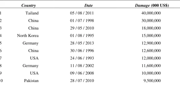
In the period from 1998 to 2009 floods and storms were considered the most costly hazards (EEA). From the Table 1.2 it is evident that the floods caused the highest economic losses over the past decades. This is an outcome from the increase of population and the growth of assets on the river floodplains.
Table 1.1: Top 10 important flood disasters for the period 1900 to 2014. (Source: EM-DAT: The OFDA/CRED International Disaster Database, Universite catholique de Louvain, Brussels, Belgium)
Country Date Nº killed
1 China July 1931 3,700,000
2 China July 1959 2,000,000
3 China July 1939 500,000
4 China 1935 142,000
5 China 1911 100,000
6 China July 1949 57,000
7 Guatemala October 1949 40,000
8 China August 1954 30,000
9 Venezuela 15 of December 1999 30,000
_____________________________________________________________________________
6
Table 1.2: The most devastating flood disasters. Top 10 at economic losses for the period 1900 to 2014. (Source: EM-DAT: The OFDA/CRED International Disaster Database, Universite catholique de Louvain, Brussels, Belgium)
Country Date Damage (000 US$)
1 Tailand 05 / 08 / 2011 40,000,000
2 China 01 / 07 / 1998 30,000,000
3 China 29 / 05 / 2010 18,000,000
4 North Korea 01 / 08 / 1995 15,000,000
5 Germany 28 / 05 / 2013 12,900,000
6 China 30 / 06 / 1996 12,600,000
7 USA 24 / 06 / 1993 12,000,000
8 Germany 11 / 08 / 2002 11,600,000
9 USA 09 / 06 / 2008 10,000,000
10 Pakistan 28 / 07 / 2010 9,500,000
At present it is not possible to prevent flood disasters, thus a comprehensive understanding of the flood phenomenon has to be considered. Thus, in 1986 the Science and Engineering Research Council (SERC) and Hydraulics Research Ltd (HR) have constructed the Flood Channel Facility (FCF) to provide a database for validating the numerical models and to enable engineers to understand the hydraulic processes involved in river flooding. Most floods originate a so-called compound channel flow, where the flow is deeper and faster in a main channel (inbank flow) and shallower and slower in lateral floodplains (overbank flow).
The European Commission adopted the Directive 2007/60/EC that aims to reduce and manage the risks that floods pose to human health, the environment, cultural heritage and economic activity. The directive applies to all types of floods and will be implemented with a preliminary assessment of the river basin’s flood risk, as well as associated coastal zones and then followed by the development of flood hazard maps and flood risk maps by 2013 (European Environmental Agency 2010).
7
Practitioners, in general, still use 1D models for assessing flow conditions in real rivers setups, where a roughness coefficient accounts for all 3D effects (Morvan etal. 2008), making it case sensitive and implicitly increasing modelling uncertainty. Recently, 2D (streamwise and lateral directions) models are being used more often. They explicitly can account for significant variations in the cross-section shape and area, which includes floodplain flow and meandering channels (Wright 2001). Despite that, the roughness coefficients still bear some uncertainty, since they have to account for all the vertical processes that are not modelled (Morvan et al. 2008). These can be relevant when secondary flow (i.e. flow circulations transverse to the main downstream flow direction also known as helical flow) is important, like the ones occurring in channel bends, floodplain/channel interactions and to a lesser extent in straight channels (Wright 2001).
Although, the use of 3D models in real river configurations is still rare, both the increase of computational capacity and the need for more physically based predictions will push forward their use in the near future. Moreover, 3D models provide more reliable estimates of bed shear stress and other more useful information, such as the three-dimensional flow field important for mixing processes (cf. Lane et al. 1999). In this context, the use of CFD commercial codes seems more probable to occur, rather than the use of research codes developed in the academia. Mainly, because the former are user-friendly and incorporate most of the turbulence closure models, starting from the simplest one- or two-equation models to a more advanced large eddy simulation (LES). It is important to notice that the majority of commercial codes stemmed from aerodynamics industrial applications. They often present additional shortcomings, like “hidden” default strategies (Knight 2013), using default values for the empirical coefficients that sometimes cannot be changed. Nevertheless, commercial models have demonstrated their ability in simulating laboratory open-channel flows, giving results in good agreement with the experiments (Morvan et al. 2002, Morvan 2005). Even so, their validation within river flow configurations is still far to be considered fully accomplished.
Even if a CFD commercial package is available, the user will have to face a critical choice about the model that should be used. The choice is usually a compromise between the accuracy of the results and the computational time required. At present, the use of LES and Direct Numerical Simulation, DNS (this one is not usually available in commercial packages), can be discarded, due to the large quantity of data to manage and to the exceptionally high computational time required. This leaves as viable alternatives the models based on Reynolds Averaged Navier-Stokes (RANS) equations coupled with a turbulence closure model. Within
_____________________________________________________________________________
8
In the context of river flow modelling, and more precisely of compound-channel flow, it is important to assess which model will have the best binomial accuracy vs. computational time.
1.2 OBJECTIVES AND METHODOLOGY
The main objectives of the present study are:
i) to provide users of commercial CFD packages modelling guidelines regarding mesh resolution and computational domain modelling approach;
ii) to provide users of commercial CFD packages a clear picture of the performance of most common RANS turbulence closure models in simulating river flows with non-negligible secondary currents;
iii) to contribute to the understanding of the relative importance of the underlying physical hypotheses implicitly enclosed in each model in the prediction of secondary flows.
To achieve these objectives 3D simulations of laboratorial compound channel flows, where turbulence data was available (Tominaga and Nezu 1991 and Azevedo et al. 2012), were performed using the commercial package ANSYS-CFX. The simulated experiments correspond to asymmetric compound channel configurations with high flow stages (relative depth, defined as the relation between the flow depth in the floodplain and the one in the main channel, equal to 0.5), since this configuration is known to produce strong secondary flow (e.g. Nezu 1994).
Since the main focus was on accuracy vs. computational time required for different turbulence closure models, it was decided to start with the less time demanding, and most used,
k- model and then continue with the use of more complex and time demanding turbulence closure models. At the end, six different turbulence models were used, which are, in increasing order of complexity (details on each model can be consulted in Chapter 2): k- model; shear stress transport model (SST) that uses a mixture of both k- and k- models; explicit algebraic Reynolds stress model coupled with an -equation and LRR-IP pressure-strain rate correlation model (EARSM); explicit algebraic Reynolds stress model coupled with a modified -equation and LRR-QI pressure-strain rate correlation model (BSL EARSM); Reynolds stress model coupled with an -equation and SSG pressure-strain rate correlation model (SSG RSM), and Reynolds stress model coupled with a modified -equation and LRR-QI pressure-strain rate correlation model (BSL RSM).
9
transport equations, identifying the relevant terms. Some corrections available in the CFD package, mostly developed for air flows, where tested and evaluated, namely the ones regarding the EARSM.
In terms of computational domain it was decided to start by modelling the entire experimental flume, specifying the exact laboratorial inlet and outlet conditions, and to use a two fluid (water + air) domain, avoiding the specification of free-surface boundary conditions. With the increase of turbulence model complexity it was necessary, due to computational time constrains, to adopt a smaller computational domain. This was accomplished by using a single phase fluid (water), being the free-surface modelled as a rigid lid with free slip conditions (see Chapter 3 for details). Also periodic boundary conditions were imposed at the inlet and outlet, allowing to shorten the length of the computational domain.
For reaching solid conclusions on the accuracy of each model and comparing different simulations it was also necessary to establish verification and validation criteria for the latter, ensuring that the turbulent velocity field was converged. For that purpose several meshes were used, starting with a coarser one and refining it locally, in the regions of interest (i.e. bottom, walls, free-surface and interface between main channel and floodplain), until reaching an acceptable convergence of the turbulent field.
1.3 THESIS OUTLINE
The present work is divided into six chapters and two appendixes. Since the results originated a sum of papers with self-contained introductions and references, and independent pagination, notation and text style, it was decided to present them in Appendix A as the original published papers.
Chapter 1 introduces the reader to the studied topic, giving a background that motivated this study, stating the main objectives and a brief description of the methodology used to accomplish them, and presenting the outline of the thesis.
In Chapter 2 a brief review of the governing equations and turbulence closure models is presented together with some problems and limitations in turbulence modelling. This chapter allows readers not familiar with turbulence closures models to have an overview of the main characteristics of the models used in the thesis.
_____________________________________________________________________________
10
Chapter 4 encloses some significant contributions concerning numerical modelling of the inbank flow in straight rectangular and trapezoidal open channels, and then the main aspects on numerical modelling of rectangular and trapezoidal compound channel flows are briefly summarised. This chapter aims to give the reader a picture of the turbulent field in compound channel flows and the different numerical approaches used previously by other authors in their simulations.
Chapter 5 summarizes the results of each individual research paper, allowing the reader to have an overall view of the link between research papers and its sequence.
Chapter 6 resumes the main conclusions and findings of this thesis and suggests topics for further research.
11
1.4 REFERENCES
Azevedo, R., Rojas-Solórzano, L. R. and Leal, J. B. 2012 Experimental characterization of straight compound-channel turbulent field. In Proc. of 2nd European IAHR Congress. 27-29 June, Munich, Germany.
Berz, G. 2000 Flood disasters: Lessons from the past – worries for the future. Proc. Inst. Civil Eng. Water and Maritime Engineering, London 142 (1), 3-8.
Directive 2007/60/EC of the European Parliament and of the Council of 23 October 2007 on the assessment and management of flood risks (Text with EEA relevance).
European Environmental Agency 2010 Mapping the impacts of natural hazards and technological accidents in Europe. An overview of the last decade. Technical report ISSN 1725-2237, 13, 1-144. European Environmental Agency Disasters in Europe: more frequent and causing more damage
(http://www.eea.europa.eu/highlights/natural-hazards-and-technological-accidents)
Hebert, P. and Ontario, B. 2013 River. Retrieved from http://www.eoearth.org/view/article/155760
Knight, D. W. 2013 River hydraulics – a view from midstream. Journal of Hydraulic Research51 (1), 2-18.
Knight, D. W. and Shamseldin, A. 2006 River basin modelling for flood risk mitigation. Taylor & Francis, Leiden.
Knight, D. W., Tang, X., Sterling, M., Shiono, K. and McGahey, C. 2010 Solving open channel flow problems with a simple lateral distribution model. In River Flow 2010, Proc. Int. Conf. on Fluvial Hydraulics, 41-48, A. Dittrich, K. Koll, J. Aberle, P. Geisenhainer, eds. Braunschweig.
Lane, S. N., Bradbrook, K. F., Richards, K. S., Biron, P. A. and Roy, A. G. 1999 The application of computational fluid dynamics to natural river channels: three-dimensional versus two-dimensional approaches. Geomorphology29 (1), 1-20.
Morvan, H. P. 2005 Channel shape and turbulence issues in flood flow hydraulics. Journal of Hydraulic Engineering, 131 (10), 862-865.
Morvan, H., Knight, D., Wright, N., Tang, X. and Crossley, A. 2008 The concept of roughness in fluvial hydraulics and its formulation in 1D, 2D and 3D numerical simulation models. Journal of Hydraulic Research46 (2), 191-208.
Morvan, H. P., Pender, G., Wright, N.G. and Ervine, D. A. 2002 Three-dimensional hydrodynamics of meandering compound channels. Journal of Hydraulic Engineering 128 (7), 674-682.
Nezu, I. 1994 Compound open-channel turbulence and its role in river environment. Keynote Address of 9th APD-IAHR Congress, Delft, The Netherlands, 1-24.
Tominaga, A. and Nezu, I. 1991 Turbulent structure in compound open-channel flows. Journal of Hydraulic Engineering 117 (1), 21-40.
CHAPTER 2
_____________________________________________________________________________
15
Contents
_____________________________________________________________________________
17
2
BASIC CONCEPTS IN TURBULENCE MODELLING
2.1 INTRODUCTION
In this chapter a brief review of the governing equations valid for constant-property (e.g. density and viscosity) Newtonian fluids and isothermal flows under a constant gravitational field are presented. A detailed review of several turbulence models used to closure the Reynolds Averaged Navier-Stokes (RANS) equations is also presented, focusing on the main assumed hypotheses that can have impact on the numerical results.
Equations in the following Subchapters use Cartesian index notation, where i = 1 is for x - direction (along the flow) and streamwise velocity component u, i = 2 is for y - direction (across the flow) and transversal velocity component v, and i = 3 is for z (orthogonal to the fluid bed) and vertical velocity component w.
2.2 GOVERNING EQUATIONS AND REYNOLDS AVERAGING
The basic system of governing equations for incompressible fluid flows is based on the conservation laws of physics:
- conservation of mass (i.e. continuity equation), - conservation of momentum (Newton’s second law).
The mass-conservation or continuity equation for an incompressible fluid can be written as (e.g. Pope 2000):
0 or 0 div i i x u z w y v x u u (2.1)
The second equation, conservation of momentum, states that the rate of change of momentum equals the sum of the forces on a fluid element. For a constant-property (e.g. density and viscosity) Newtonian fluid and isothermal flow under a constant gravitational field can be written (e.g. Pope 2000):
i j i j i j i j i f x u x x p x u u t u
1 (2.2)
where p is instantaneous pressure field, ρ is the fluid density, ν is the fluid kinematic viscosity and fi are body forces. Equations (2.2) are known as Navier-Stokes equations for
_____________________________________________________________________________
18
Equations (2.2) completely describe the laminar-turbulent field and may, in principle, be solved directly in so called direct numerical simulation (DNS). However, the numerical solution is extremely difficult, since the significantly different length and time scales in a turbulent field need to be resolved, and thus the stable solution requires such a fine mesh resolution that the computational effort grows rapidly with increasing Reynolds number. Thus, practically in most turbulent flows the flow-field variables are decomposed into the mean and fluctuating parts. This process is known as the Reynolds decomposition and can be expressed as:
' i i
i
U
u
u
(2.3)where ui is the instantaneous velocity component,
'
i
u is the fluctuating part for which ui' 0 and
i
U
is the mean velocity. Note that this mean value should be obtained from classic statistics knowing the probability density function of the random variable (velocity field). However, a very common approach, also adopted here, is to consider that the flow is statistically stationary (i.e. all statistics are invariant under a shift in time). This allows estimating the statistical mean by performing a average (over a time interval). For statistically stationary flows, the time-averaged value tends to the statistical mean value as the used time interval tends to infinity (e.g. Pope 2000).Substituting the decomposition (2.3) for velocity and pressure into the continuity and momentum equations (Eqs. (2.1) and (2.2
)
), and then by averaging all the terms in the equations and taking into account that ui'0 and Ui Ui , the Reynolds averaged Navier-Stokes equations (RANS) for constant-property Newtonian fluids are obtained (e.g. Pope 2000):0
i ix
U
(2.4) j j i j i j i j i j ix
u
u
x
U
x
x
P
x
U
U
t
U
' '1
(2.5)For brevity, the overbars indicating the averaged values are dropped from Ui and P from here
19
correlation matrix between fluctuating components of the velocity field, is also denominated the Reynolds stress tensor.
2.3 PROBLEMS AND LIMITATIONS IN TURBULENCE MODELLING
Turbulence can either be resolved or modelled. Resolving implies proper solution of the governing equations (at all scales) with no modelling or empirical assumptions. Modelling implies a solution that uses some degree of approximation and empiricism.
There are three levels of resolving turbulence: fully resolved, partially resolved, and unresolved. Direct Numerical Simulation (DNS) is one technique that attempts to fully resolve turbulent flow by solving the Navier-Stokes equations at all length and time scales. In DNS turbulence or empirical models are not required.
The ample variation in length and time scales is an important characteristic of turbulent flows which is in part responsible for the difficulty encountered in the numerical and theoretical analysis of turbulent flows. The largest length scales (eddy sizes), given by L, in the flow account for most of the transport of momentum and energy. The size of these eddies is constrained by the physical boundaries of the flow. Thus, for compound channel flow the largest eddies can have the size of the channel width.
Kinetic energy from large eddies is transferred to the smaller eddies during the cascading process until it is dissipated into heat (Pope 2000). As we approach smaller and smaller length scales, the viscous effects become more important. Thus, the size of the smallest eddies, η, at which this energy is dissipated depends on the dissipation rate, ε, and viscosity, ν, and is defined as:
4 / 1 3
(2.6)
This length scale is called the Kolmogorov length scale and it characterizes the smallest dissipative eddies. Therefore, it corresponds to the smallest length scale needed to properly resolve turbulent flow.
The time scale, τ, of the smallest eddies is:
2 / 1
(2.7)
_____________________________________________________________________________
20
Reynolds number of 105, the ratio L/η is proportional to 1015/4. Thus, to resolve the entire range
of length scales in 3D turbulent flow, we would need a computational domain that consists of at least 1010 grid points. The amount of information resulting from such simulation would exceed
the capacity of any existing computer. This becomes even clearer when the unsteady, transient nature of turbulence is considered. Thus, the problem with DNS is that it consumes enormous computational resources since the grid resolution must be on the order of the Kolmogorov scales as indicated in previous paragraphs. Currently, DNS is a research tool and is only feasible for simple flows at lower Reynolds numbers (Kim etal. 1987).
Large Eddy Simulation (LES) attempts to partially resolve turbulence. The fundamental idea is that the small scales of turbulence (close to the Kolmogorov scales) can be modelled by a subgrid model, while the larger scales are resolved by the governing equations. Grid resolution is on the order of the turbulent scale that wants to be solved, thus in LES the computational demands are considerably smaller than in DNS. The LES has become more and more popular and shows good results when compared to experimental data (e.g. Thomas and Williams 1995, Cater and Williams 2008, Stoesser 2010, Kara etal. 2012). Nevertheless, its application to real setups is still impractical, due to the exceptionally high computational effort required.
The most practical and still the most popular method of dealing with turbulence is that based on RANS equations. Only mean flow quantities are resolved. In the RANS method, all scales of turbulence are modelled; grid resolution is in the order of the mean flow scale - not a turbulent scale. This offers huge computational savings when compared to both DNS and LES. The complexity of RANS models ranges from purely algebraic or zero-equation models to a more complex Reynolds stress models.
Reynolds stresses appearing in RANS have to be related to the mean motion itself before the equations can be solved, since the number of unknowns and number of equations must be equal. From equations (2.4) and (2.5) we have 10 unknowns (P, U1, U2, U3, and six Reynolds
stresses ui'u'j ) and only 4 equations, which configures an unclosed mathematical problem. The
absence of these additional equations is often referred to the turbulence closure problem. To close these equations, i.e. have the same number of equations and unknowns, extra equations are introduced through the different turbulence models, which will be described in the next subchapters.
2.4 EDDY VISCOSITY MODELS
21
laminar flow, the turbulent stresses are assumed to be proportional to the mean velocity gradients (e.g. Nezu and Nakagawa 1993). The Reynolds stress tensor is then related to the mean flow field through:
ij i j j i t j i k x U x U u
u
3 2 ' ' (2.8)
where νt is the eddy viscosity; δijis the Kronecker delta (δij = 1 for i = j; and δij = 0 for i≠j); and
k is the turbulence kinetic energy, defined as k ui'ui' 2.
As will be shown in later subchapters, the primary goal of many turbulence models is to find some estimation for the eddy viscosity to model the Reynolds stresses. These may range from the relatively simple algebraic models, to the more complex models such as the k-ε model, where two additional transport equations are solved in addition to the mean flow equations. Here only two-equation models will be presented (more details of zero- or one-equation models can be found in standard books like Rodi (1993), Pope (2000) or Wilcox (2006).
The two-equation models are the simplest complete models, since these models provide independent transport equations for both variables, the turbulence kinetic energy and the turbulence length scale, or some equivalent parameter.
Kolmogorov (1942) and Prandtl (1945) suggested determining the distribution of k by solving a model transport equation forthis quantity, which can be obtained by introducing the Reynolds decomposition in the Navier-Stokes equations, multiplying by the velocity and taking time-average of the resulting equation (e.g. Pope 2000). The resulting transport equation for k
can be written as:
of n dissipatio of rate ' ' production e turbulenc ' ' of transport Turbulent ' ' ' ' of transport Convective of change of Rate ν ρ 2 k j i j i P j i j i k j j i i k i i k x u x u x U u u p u u u x x k U t k (2.9)
Equation (2.9) is the exact k-equation and is of no use in the turbulence model since new unknown correlations appear in the turbulent transport and dissipation terms. To obtain a closed set of equations, model assumptions must be introduced for these terms. Thus, turbulent transport term is often modelled with a gradient-diffusion concept (2.10). The reader should keep in mind that gradient-diffusion hypothesis is applicable to high Reynolds number flows and is not valid in certain flow regions, such as the viscous sublayer near walls.
_____________________________________________________________________________ 22 i k t j j i
x
k
p
u
u
u
' ' ' '2
(2.10)where σk is the turbulent Schmidt number that does not have a universal value and empirical
values have been used in different studies in the range of 0.2 - 1.3 (Tominaga and Stathopoulos 2007). The selected value of σk has a significant effect on the prediction of the results. Thus,
Tominaga and Stathopoulos (2007) recommended that σk should be determined by considering
the dominant flow structures for each case. However, σk generally takes value around 1.0 (e.g.
Nezu and Nakagawa 1993, Pope 2000, Rodi 1993).
Taking into account the above mentioned assumptions in (2.8) and (2.10), equation (2.9) reads: k P j i i j j i t k i k t i k i i k x U x U x U x k x x k U t k of n dissipatio of rate production e turbulenc of transport Turbulent convection by of Transport of change of Rate (2.11)
The choice of the second variable in two-equation models is arbitrary and many proposals have been presented. Thus, Davidov (1961), Harlow and Nakayama (1968) and Jones and Launder (1972) suggested an equation for the dissipation rate ε = k3/2/l, being l a turbulence
length-scale; Rotta (1951) proposed an equation for kl; Kolmogorov (1942) an equation for the turbulence frequency ω = k1/2/l; Saffman (1970) an equation for turbulence vorticity ω2 = k/l2
and Speziale et al. (1992) an equation for the turbulent time-scale τ = l/k1/2. Two of the most
popular dependent variables for the second variable have been the dissipation rate ε and the specific dissipation rate ω. These models will be discussed in more details since they have been applied to calculate compound channel flow in this study (see Research Paper II).
The k-ε model is the best-known two-equation turbulence model and is incorporated in most commercial CFD codes. The most used formulation of the k-ε model, referred as the “standard”
k-ε model, is of Jones and Launder (1972). Those authors proposed the following transport equation for the dissipation rate:
of transport Turbulent ofrate and dissipation Production 2 1 convection by of Transport of change of Rate i t i i i x x C P C k x U t (2.12)
23
t Ck2 (2.13)
It should be referred that equation (2.12) is not the exact transport equation for ε, but rather an entirely empirical equation that can account better for the fact that ε is determined by the large-scale motions (energy cascade) instead of motions in the dissipative range (cf. Pope 2000). The k-ε model involves the five empirical constants Cμ, Cε1, Cε2, σkand σε. Their standard
values for open-channel flows are presented in the Table 2.1. The choice of these constants is based on the compatibility of the model to the logarithmic velocity distribution near the wall in channel flows with Von Kármán constantκ = 0.41 (Nezu and Nakagawa 1993).
In open-channel flows, vertical fluctuations, w, are damped by the free-surface, which
results in νt approaching to zero near the free-surface (Nezu and Nakagawa 1993). This surface
damping can be accounted for in the k-ε model by decreasing Cμ near the free-surface by means of damping functions, or surface-proximity function (Celik and Rodi 1984).
Table 2.1: Values of the constants in the k-ε model for open-channel flows (Nezu and Nakagawa 1993)
Cμ Cε1 Cε2 σk σε
0.09 1.44 1.92 1.2 1.2
Another popular two-equation model is the k–ω model (being the turbulence frequency ω = ε/k), which will be presented here in the form given by Wilcox (1988). The k-ω model solves the k-transport equation (2.11) and a transport equation for ω, instead of the ε-equation (2.12). The k-transport equation, re-written replacing ε = kω, and the transport equation for ω can be written (Wilcox 1988):
k P x k x x k U t k i k t i i i ' (2.14) 2 P k x k x x k U t i t i i i (2.15)
and the eddy viscosity is given:
tk
(2.16)The k-ω model involves five empirical constants β’, β, α, σkand σω. Their standard values are
_____________________________________________________________________________
24
Table 2.2: Values of the constants in the k- ω model (Wilcox 1988).
β’ β α σk σω
0.09 0.075 5/9 2 2
Another two-equation model was proposed by Menter (1994), which combines the best behaviour of the k-ε and k-ω models (k-ω performs better near the wall region and k-ε performs better in the fully turbulent region). This model is implemented into ANSYS CFX and it is known as the Baseline (BSL) k-ω model. This model will be discussed here in more details, since it was used for the calculations in the present study (Research Papers III and IV).
The BSL model proposed by Menter (1994) suggested a hybrid model using a transformation of the k-ε model into k-ω model in the near-wall region and the standard k-ε model in the fully turbulent region far from the wall. Thus, Wilcox model (Eq. (2.14)) is multiplied by a “blending function” F1 and the transformed k-ε model by a function (1-F1). Close to the walls the blending
function F1 is equal to one (leading to a standard ω- equation) and decreases to a value of zero
outside the boundary layer (corresponding to the standard ε- equation). The blending functions are used to achieve a smooth transition between the two models, yielding to the BSL model:
i i i t i i i x x k F P k x k x x k U t 2 1 2 3 3 3 2 1 (2.17)An extra source term, called cross-diffusion term, appears on the right hand side (RHS), which arises during the transformation. The model constants, Φ3(being Φeither , or ), are
related through a linear combination of a set of constants Φ1 and Φ2 (where subscripts 1 and 2
correspond to constants of k- and of k- models presented in Table 2.2 and Table 2.1,
respectively):
2 1 1
1
3 (1 )
F F (2.18)
Blending function F1 is defined as:
4 1 1tanhargF (2.19) with 2 2 2 ' 1 4 , 500 , max min arg z CD k z z k k (2.20)
25 10 2 10 , 2 max i i k x x k CD (2.21)
For completeness, all BSL constants are listed again in the Table 2.3.
Table 2.3: Values of the coefficients in the BSL k-ω model.
Φ1 β’ β1 α1 σk1 σω1
0.09 0.075 5/9 2 2
Φ2 β’ β2 α2 σk2 σω2
0.09 0.0828 0.44 1 1/0.856
Another two-equation model which has become very popular is the Shear Stress Transport (SST) k-ω model proposed also by Menter (1993). The k-ω based SST model accounts for the transport of the turbulent shear stresses, according to modifications introduced to the original k -ω model by Menter. One of these modifications is referred to obtain a limiter for the formulation of the eddy viscosity, given by:
1 2
1ω,
maxa SF
k a
t
(2.22)
where 𝑆 = √2𝑆𝑖𝑗𝑆𝑖𝑗, a1 is a constant and F2 is a blending function similar to F1.
22 2 tanharg
F (2.23) ω ν 500 , ω 2 max arg 2 ' 2 z z k (2.24)
A disadvantage of standard two-equation turbulence models is the excessive production of turbulence kinetic energy, P. Therefore, another formulation of limiters for the production term in the turbulence equations was suggested by Menter (1994) as:
,10β ω
minP 'k
P (2.25)
In conclusion, two-equation models have proven that they perform reasonably well for a wide range of flows of engineering interest, with some limitations that may be accounted with the use of special bounding or damping functions. Their major advantage is the simplicity, and the low computational cost compared to more complex models, such as RSM or LES.