Universidade do Minho Escola de Engenharia Departamento de Informática
Master Course in Computing Engineering
Christopher Borges Costa
Development of an integrated computational platform for
metabolomics data analysis and knowledge extraction
Master dissertation
Supervised by: Miguel Francisco de Almeida Pereira da Rocha
A C K N O W L E D G E M E N T S
Queria agradecer ao meu orientador e co-orientador, o Professor Miguel Francisco de Almeida Pereira da Rocha e o Professor Marcelo Maraschin, pela ajuda e apoio que deram para a realização desta dissertação.
Agradeço também a todas as pessoas que de alguma forma contribuíram para a realização deste projecto.
A B S T R A C T
In the last few years, biological and biomedical research has been generating a large amount of quan-titative data, given the surge of high-throughput techniques that are able to quantify different types of molecules in the cell. While transcriptomics and proteomics, which measure gene expression and amounts of proteins respectively, are the most mature, metabolomics, the quantification of small com-pounds, has been emerging in the last years as an advantageous alternative in many applications.
As it happens with other omics data, metabolomics brings important challenges regarding the ca-pability of extracting relevant knowledge from typically large amounts of data. To respond to these challenges, an integrated computational platform for metabolomics data analysis and knowledge ex-traction was created to facilitate the use of several methods of visualization, data analysis and data mining.
In the first stage of the project, a state of the art analysis was conducted to assess the existing meth-ods and computational tools in the field and what was missing or was difficult to use for a common user without computational expertise. This step helped to figure out which strategies to adopt and the main functionalities which were important to develop in the software. As a supporting framework, R was chosen given the easiness of creating and documenting data analysis scripts and the possibility of developing new packages adding new functions, while taking advantage of the numerous resources created by the vibrant R community.
So, the next step was to develop an R package with an integrated set of functions that would allow to conduct a metabolomics data analysis pipeline, with reduced effort, allowing to explore the data, apply different data analysis methods and visualize their results, in this way supporting the extraction of relevant knowledge from metabolomics data.
Regarding data analysis, the package includes functions for data loading from different formats and pre-processing, as well as different methods for univariate and multivariate data analysis, including t-tests, analysis of variance, correlations, principal component analysis and clustering. Also, it includes a large set of methods for machine learning with distinct models for classification and regression, as well as feature selection methods. The package supports the analysis of metabolomics data from infrared, ultra violet visible and nuclear magnetic resonance spectroscopies.
The package has been validated on real examples, considering three case studies, including the analysis of data from natural products including bees propolis and cassava, as well as metabolomics data from cancer patients. Each of these data were analyzed using the developed package with differ-ent pipelines of analysis and HTML reports that include both analysis scripts and their results, were generated using the documentation features provided by the package.
R E S U M O
Nos últimos anos, a investigação biológica e biomédica tem gerado um grande número de dados quan-titativos, devido ao aparecimento de técnicas de alta capacidade que permitem quantificar diferentes tipos de moléculas na célula. Enquanto a transcriptómica e a proteómica, que medem a expressão genética e quantidade de proteínas respectivamente, estão mais desenvolvidas, a metabolómica, que tem por definição a quantificação de pequenos compostos, tem emergido nestes últimos anos como uma alternativa vantajosa em muitas aplicações.
Como acontece com outros dados ómicos, a metabolómica traz importantes desafios em relação à capacidade de extracção de conhecimento relevante de uma grande quantidade de dados tipicamente. Para responder a esses desafios, uma plataforma computacional integrada para a análise de dados de metabolómica e extracção de informação foi criada para facilitar o uso de diversos métodos de visualização, análise de dados e mineração de dados.
Na primeira fase do projecto, foi efectuado um levantamento do estado da arte para avaliar os métodos e ferramentas computacionais existentes na área e o que estava em falta ou difícil de usar para um utilizador comum sem conhecimentos de informática. Esta fase ajudou a esclarecer que estratégias adoptar e as principais funcionalidades que fossem importantes para desenvolver no software. Como uma plataforma de apoio, o R foi escolhido pela sua facilidade de criação e documentar scripts de análise de dados e a possibilidade de novos pacotes adicionarem novas funcionalidades, enquanto se tira vantagem dos inúmeros recursos criados pela vibrante comunidade do R.
Assim, o próximo passo foi o desenvolvimento do pacote do R com um conjunto integrado de funções que permitem conduzir um pipeline de análise de dados, com reduzido esforço, permitindo explorar os dados, aplicar diferentes métodos de análise de dados e visualizar os seus resultados, desta maneira suportando a extracção de conhecimento relevante de dados de metabolómica.
Em relação à análise de dados, o pacote inclui funções para o carregamento dos dados de diver-sos formatos e para pré-processamento, assim como diferentes métodos para a análise univariada e multivariada dos dados, incluindo t-tests, análise de variância, correlações, análise de componentes principais e agrupamentos. Também inclui um grande conjunto de métodos para aprendizagem au-tomática com modelos distintos para classificação ou regressão, assim como métodos de selecção de atributos. Este pacote suporta a análise de dados de metabolómica de espectroscopia de infravermel-hos, ultra violeta visível e ressonância nuclear magnética.
O pacote foi validado com exemplos reais, considerando três casos de estudo, incluindo a análise dos dados de produtos naturais como a própolis e a mandioca, assim como dados de metabolómica de pacientes com cancro. Cada um desses dados foi analisado usando o pacote desenvolvido com
diferentes pipelines de análise e relatórios HTML que incluem ambos scripts de análise e os seus resultados, foram gerados usando as funcionalidades documentadas fornecidas pelo pacote.
C O N T E N T S Contents i 1 I N T R O D U C T I O N 1 1.1 Context 1 1.2 Objectives 2 1.3 Dissertation organization 2 2 S TAT E O F T H E A R T 5 2.1 Techniques 5
2.1.1 Nuclear Magnetic Resonance 5
2.1.2 Infrared Spectroscopy 6
2.1.3 Ultraviolet-visible 8
2.2 Workflow of a metabolomics experiment 9
2.2.1 Preprocessing 10
2.2.2 Metabolite identification and quantification 12
2.2.3 Univariate data analysis 13
2.2.4 Unsupervised Methods 14
2.2.5 Supervised Methods: machine learning 15
2.2.6 Feature Selection 18
2.3 Databases of metabolomics data 19
2.3.1 HMDB 19
2.3.2 MetaboLights 19
2.4 Available free tools for metabolomics 20
2.5 Data integration 21
3 D E V E L O P M E N T 23
3.1 Development strategy and tools 23
3.2 Dataset structure and creation 24
3.2.1 Dataset structure 24
3.2.2 Reading data and creating datasets 26
3.2.3 Conversion to/from other packages 26
3.3 Exploratory Analysis 27
3.3.1 Statistics 27
3.3.2 Graphics 27
3.4 Preprocessing 28
Contents
3.4.2 Spectral Corrections 28
3.4.3 Missing Values 30
3.4.4 Data normalization, transformation and scaling 30
3.4.5 Flat pattern filtering 31
3.5 Univariate data analysis 31
3.6 Unsupervised multivariate analysis 33
3.6.1 Dimensionality reduction 33
3.6.2 Clustering 35
3.7 Machine Learning and Feature Selection 37
4 C A S E S T U D I E S 41 4.1 Propolis 41 4.1.1 Introduction 41 4.1.2 NMR data 42 4.1.3 UV-Vis data 52 4.2 Cachexia 55 4.2.1 Introduction 55 4.2.2 Concentrations data 55 4.3 Cassava 61 4.3.1 Introduction 61 4.3.2 IR data 61 5 C O N C L U S I O N S A N D F U T U R E W O R K 65 ii
L I S T O F F I G U R E S
Figure 1 General workflow of a metabolomics experiment 10
Figure 2 Example of a peak overlap 13
Figure 3 Low-level fusion example 22
Figure 4 Intermediate-level fusion example 22
Figure 5 Representation of the structure of the data in a dataset 25
Figure 6 Boxplot for a subset of the metabolites in a dataset 27
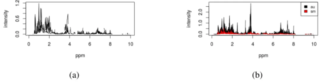
Figure 7 (a) Plot of plot.spectra.simple function from a subset of a dataset with 5 samples. (b) Plot of plot.spectra function from a subset of a dataset with 20 samples and colored by a metadata variable. 28
Figure 8 t-test, fold change and volcano plot from a metabolite’s concentrations dataset 33
Figure 9 (a) PCA scree plot generated by pca.screeplot function. (b) 2D PCA scores plot (PC1 and PC2) from the function pca.scoresplot2D. (c) 3D PCA scores plot (PC1, PC2 and PC3) from the function pca.scoresplot3D. (d) PCA Bi-plot generated by pca.biBi-plot function. 35
Figure 10 (a) Dendrogram with colored leaves from dendrogram.plot.col function. (b) k-means plot showing four clusters. 36
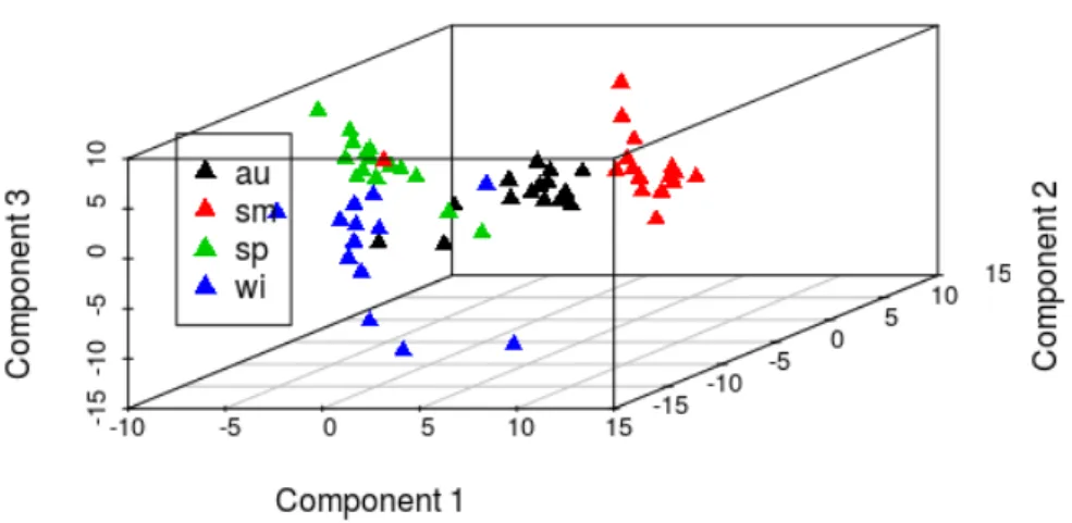
Figure 11 3D scatter plot of the first 3 components from a PLS model. 39
Figure 12 Dendrogram with season color labels. 44
Figure 13 k-meansplot with four clusters. 44
Figure 14 PCA scores plot (PC1 and PC2) grouped by seasons. 45
Figure 15 PCA scree plot. 46
Figure 16 PCA scores plot (PC1 and PC2) grouped by the clusters from k-means. 46
Figure 17 3D plot of the first 3 components of the pls model with seasons metadata 50
Figure 18 3D plot of the first 3 components of the pls model with agroregions
meta-data 51
Figure 19 Dendrogram with regions as label colors. 53
Figure 20 PCA 2D scores plot (PC1 and PC2) grouped with seasons metadata. 53
Figure 21 t-tests plot from the pipeline. 56
Figure 22 Fold change plot from the cachexia dataset. 57
Figure 23 Volcano plot from the t-tests and fold change. 58
Figure 24 Resulting dendrogram from hierarchical clustering. 58
Figure 25 Scree plot. 59
List of Figures
Figure 27 Resulting dendrogram from hierarchical clustering of cassava dataset with replicates. 63
Figure 28 2D plot score (PC1 and PC2) from cassava data without the replicates and
PPDs metadata. 63
L I S T O F TA B L E S
Table 1 Applications of NMR, IR and UV-Vis spectroscopies 8
Table 2 Databases of metabolomics data 20
Table 3 Available free tools for metabolomics data 21
Table 4 Resampling methods 37
Table 5 Some models with their tuning parameters. 38
Table 6 ANOVA results with seasons metadata. 43
Table 7 Members of the clusters of k-means. 45
Table 8 Classification models result with seasons metadata. 47
Table 9 Classification models result with agroregions metadata. 47
Table 10 Full results using pls with different number of components with seasons
metadata. 48
Table 11 Full results using pls with different number of components with agroregions
metadata. 49
Table 12 Confusion matrix of the pls model with seasons metadata 49
Table 13 Confusion matrix of the pls model with agroregions metadata 50
Table 14 Variable importance of the pls model with seasons metadata 51
Table 15 ANOVA results with seasons metadata. 52
Table 16 Classification models result with seasons metadata. 54
Table 17 Classification models result with regions metadata. 54
Table 18 Classification models result with years metadata. 54
Table 19 t-Tests results ordered by p-value. 56
Table 20 Fold change results ordered bylog2of fold change values from the data. 57
Table 21 Classification results. 60
Table 22 ANOVA results using the cassava dataset with no replicates with varieties
metadata. 62
Table 23 ANOVA results using the cassava dataset with no replicates with Postharvest Physiological Deterioration (PPD) metadata. 62
L I S T O F F O R M U L A S
1 Expected accuracy . . . 16
2 Kappa statistic. . . 16
3 Logarithmic transformation . . . 30
4 Cubic root transformation. . . 30
5 Auto scaling . . . 31
6 Pareto scaling . . . 31
7 Range scaling . . . 31
A C R O N Y M S
ANN Artificial Neural Network.18,19
ANOVA Analysis of Variance. 15,16,33,34,43,51,52,61
BATMAN Bayesian AuTomated Metabolite Analyser for NMR spec-tra. 13
COW Correlation Optimized Warping.13
CSV Comma Separated Values. 28
CT Computed Tomography. 55
DA Discriminant Analysis.9
DXA Dual energy X-ray Absortiometry.55
FC Fold Change.16,56
FDR False Discovery Rate. 16
FTIR Fourier-Transform Infrared. 8,20
GA Genetic Algorithms.20,65
HCA Hierarchical Cluster Analysis.16,22,36,37
HLF High-Level Fusion.22
HRMAS High Resolution Magic Angle Spinning.7
HSD Honest Significance Difference.15,16,34,43,51,52,61
IDE Integrated Development Environment.26
ILF Intermediate-Level Fusion. 22,23
iPLS interval Partial Least Squares.20
IR Infrared.4,11,13,18,22,23
kNN k-Nearest Neighbors.18,32
Acronyms
LLF Low-Level Fusion. 22,23
LR Linear Regression. 9
LV Latent Variables.18
MCMC Markov Chain Monte Carlo.14
MRI Magnetic Resonance Imaging.55
mRNA Messenger Ribonucleic Acid. 3
MS Mass Spectrometry.22,65
MSC Multiplicative Scatter Correction.13,22,30,31
NMR Nuclear Magnetic Resonance. 4,7,8,11–14,18, 21–23,
28,41,42,52,55,65
OSC Orthogonal Signal Correction.9
PC Principal Component.53
PCA Principal Component Analysis.16,18,22,34,45,46,53,
59,63
PLS Partial Least Squares. 18,20,39
PLS-DA Partial Least Squares - Discriminant Analysis. 18,22
PLS-r Partial Least Squares - regression.18
PPD Postharvest Physiological Deterioration.41,61–63
QDA Quadratic Discriminant Analysis.9
RFE Recursive Feature Elimination. 20,40
RIPPER Repeated Incremental Pruning to Produce Error Reduc-tion.19
RMSE Root Mean Square Error.38
SIMCA Soft Independent Modeling of Class Analogy.18
SVD Singular Value Decomposition. 34
SVM Support Vector Machine. 18,19,22,60
TOCSY Total Correlation Spectroscopy. 14
TSP, 0.024 g% Trimethylsilyl Propionate Sodium salt.42
TSV Tab Separated Values.28
Acronyms
1
I N T R O D U C T I O N
1.1 C O N T E X T
Metabolomics can be defined as the identification and quantification of all intra- cellular and extra-cellular metabolites with low molecular mass. It is one of the so called omics technologies that have recently revolutionized the way biological research is conducted, offering valuable tools in func-tional genomics and, more globally, in the characterization of biological systems (Nielsen and Jewett,
2007). Indeed, these technologies allow the global measurement of the amounts of different molecules (e.g. Messenger Ribonucleic Acid (mRNA)in transcriptomics, proteins in proteomics) providing nu-merous applications in biological discovery, biotechnology and biomedical research. Applications of metabolomics data include studying metabolic systems, measuring biochemical phenotypes, un-derstanding and reconstructing genetic networks, classifying and discriminating between different samples, identifying biomarkers of disease, analyzing food and beverage, studying plant physiology, providing for novel approaches for drug discovery and development, among others (Nielsen and Jew-ett,2007;Villas-Boas et al.,2007;Mozzi et al.,2012).
However, to achieve these goals, metabolomics data also bring important new challenges regarding the capability of extracting relevant knowledge from typically large amounts of data (Varmuza and Filzmoser,2009). Indeed, omics data have promoted the development and adaptation of numerous methods for data analysis. Unlike transcriptome and proteome technologies that are based in the anal-ysis of biopolymers with any biochemical similarity, metabolites have a large variance in chemical structures and properties, making difficult the development of high-throughput techniques and there-fore reducing the number of molecules that can adequately be measured in a sample (Villas-Boas et al.,
2007). This also implies a higher variety of techniques to be able to span all applications.
In order to respond to the challenges created by the data analysis of metabolomics data, a script based software was developed to address a wide variety of common tasks on metabolomics data analysis, providing a general workflow that can be adapted for specific case studies. This package includes tools for the visual exploration and preprocessing of the data, and further analysis to try to discover significant features regarding the type of the data with a wide variety of univariate and multivariate statistical methods, as well as machine learning and feature selection algorithms.
Chapter 1.I N T R O D U C T I O N
There are a few techniques to obtain metabolomics data. In this work, three techniques will be the main focus: Nuclear Magnetic Resonance (NMR),Infrared (IR)andUltraviolet-visible (UV-vis)
spectroscopies. Those will be explained later in more detail.
1.2 O B J E C T I V E S
Given the context described above, the main aim of this work will be the design and development of an integrated computational platform for metabolomics data analysis and knowledge extraction. The work will address the exploration and integration of data from distinct experimental techniques, focusing onNMR,UV-vis, andIR.
More specifically, the work will address the following scientific/technological goals:
• To design adequate pipelines for data analysis adapted to the distinct experimental techniques and analysis purposes.
• To implement data analysis methods for metabolomics data, taking advantage of existing open-source software tools, pursuing the development of new methods when needed.
• To design and implement specific machine learning and feature selection algorithms for the analysis of metabolomics data.
• To validate the proposed algorithms with case studies from literature and others of interest in the analysis of the potential of natural products, including for instance propolis or cassava samples.
• To write scientific publications with the results of the work.
1.3 D I S S E R TAT I O N O R G A N I Z AT I O N
This dissertation is divided in five chapters. This first chapter made a brief introduction to the theme of this dissertation and defines the objectives proposed with this work.
On the next chapter, the state of the art regarding metabolomics is covered, mentioning the existing techniques for metabolomics data acquisition, the workflow of a metabolomics experiment and data analysis with all its steps, the databases and free tools available for metabolomics, an overview of the main methods for data analysis (both univariate and multivariate) and a description of data integration and existing methods.
The third chapter describes the process of software development to reach the proposed package in R. All the software features are described, as well as the development strategy and the tools that were used, together with the details of the methods developed for each step of the metabolomics workflow. In the fourth chapter, three case studies were analyzed with the software developed. The details of each case study, the respective results, as well as the interpretation of those results are included in the chapter.
1.3. Dissertation organization
Finally, the last chapter contains the conclusions of the work done and the proposals for future work.
2
S TAT E O F T H E A R T
In this chapter, the state of the art of the metabolomics field will be covered. This includes the description of the main techniques and their characteristics, and the available methods for data pre-processing and analysis. The workflow of data analysis for a metabolomics experiment will be fully covered, which includes the preprocessing, metabolite identification and quantification, univariate and multivariate data analysis, the databases and free tools existent for metabolomics and data integration.
2.1 T E C H N I Q U E S
2.1.1 Nuclear Magnetic Resonance
NMR spectroscopy is one of the most frequently employed experimental techniques in the analysis of the metabolome. It allows identifying metabolites in complex matrices in a non-selective way, providing a metabolic characterization of a given cell or tissue sample. The 1D- and 2D-NMR ex-perimental approaches are useful for structure characterization of compounds and have been applied for the analysis of metabolites in biological fluids and cells extracts. NMRspectroscopy is a robust and non-destructive sample technique, relatively inexpensive after the initial high costs of installation, also useful for quantification of metabolites in biological samples. The main drawbacks are its poor sensitivity and large sample requirement that can be an obstacle in some situations (Rochfort,2005). Some variants (e.g. High Resolution Magic Angle Spinning (HRMAS) NMR) overcome some of these limitations.
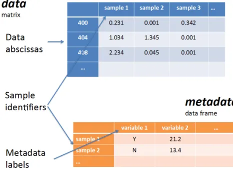
NMRprovides a spectrum with the chemical shifts in the x-axis and the intensities of the signal in the y-axis. These data are typically stored in a matrix where the chemical shifts and classification labels are the columns, and the samples are the lines (or the reverse). In this form, the data are ready to be pre-processed, analyzed and interpreted.
As said above,NMRis one of the most popular techniques employed on metabolomics experiments, so it has a lot of applications in a wide range of areas (Table1). It was used, for example, to determine the metabolic fingerprint and pattern recognition of silk extracts from seven maize landraces cultivated in southern Brazil (Kuhnen et al.,2010), predict muscle wasting (Eisner et al.,2010), identify farm
Chapter 2.S TAT E O F T H E A R T
origin of salmon (Martinez et al.,2009) or to classify Brazilian propolis according to their geographic region (Maraschin et al.,2012).
2.1.2 Infrared Spectroscopy
Infrared spectroscopy is a technique based on the vibrations of the atoms in a molecule. An infrared spectrum is commonly obtained by passing infrared radiation through a sample and determining what fraction of the incident radiation is absorbed at a particular energy. The energy at which any peak in an absorption spectrum appears corresponds to the frequency of vibration of a part of a sample molecule. The infrared spectrum can be divided into three main regions: the far-infrared (<400 cm−1), the mid-infrared (4000–400 cm−1) and the near-infrared (13 000–4000 cm−1).
The most significant advances in infrared spectroscopy have come about as a result of the intro-duction of Fourier-transform spectrometers. This type of instrument employs an interferometer and exploits the well-established mathematical process of Fourier-transformation. Fourier-Transform In-frared (FTIR)spectroscopy has dramatically improved the quality of infrared spectra and minimized the time required to obtain data. With the advantage of being simpler and less expensive, infrared spectroscopy can provide a complementary view of that provided byNMR.
There are many applications where infrared spectroscopy, usually in association with multivariate statistical methods, has been used with good results (Table1). In the food and beverage area, infrared spectroscopy was used to measure milk composition (Aernouts et al.,2011) and detect and quantify milk adulteration (Santos et al.,2013), classify beef samples according to their quality (Argyri et al.,
2010), compare metabolomes of transgenic and non-transgenic rice (Eymanesh et al.,2009), discrim-inate between different varieties of fruit vinegars (Liu et al.,2008), monitor spoilage in fresh minced pork meat (Papadopoulou et al.,2011) and predict different beer quality parameters (Polshin et al.,
2011).
Regarding the biological and medical fields infrared spectroscopy has achieved successful results, for instance in differentiating mild sporadic Alzheimer’s disease from normal aging of blood plasma samples (Burns et al.,2009), differentiating strains of bacteria (Kansiz et al.,1999;Preisner et al.,
2007) and yeasts (Cozzolino et al.,2006), and in discriminating different plant populations and the effects of environmental changes (Khairudin and Afiqah,2013).
2.1. Techniques
Reference Description Techniques Preprocessing Analysis
Acevedo et al.
(2007)
Discriminate wines
denomina-tion of origin UV-Vis Mean centering
SIMCA, SIMCA, KNN, ANNs, PLS-DA
Urbano et al.
(2006) Classification of wines UV-Vis First derivative SIMCA
Pereira et al.
(2011) Predict wine age UVV
Mean centering, Smoothing, 1st and 2nd derivative, MSC, SNV, OSC
PLS-r
Barbosa-García et al.(2007)
Distinguish between classes of
tequila UV-Vis
Derivative, centering of
columns PLS-DA
Anibal et al.
(2009)
Detect Sudan dyes (4 types) in
commercial spices UV-Vis Mean centering KNN, SIMCA, PLS-DA
Kruzlicová et al.
(2008)
Classification of different sorts of olive oil and pumpkin seed oil, supplemented with oil qual-ity
UV-Vis, IR None
LDA, Quadratic Dis-criminant Analysis (QDA), KNN, Linear Regression (LR), ANNs
Kumar et al.
(2013)
Clustering and classification of
tea varieties UV-Vis-NIR Normalization PCA, K-Means, ANNs
Souto et al.
(2010)
Classification of brazilian
ground roast coffee UV-Vis None SIMCA, LDA
Thanasoulias et al.(2003)
Discrimination of blue ball
point pen inks UV-Vis Normalization, Log
PCA, K-Means, Discrim-inant Analysis (DA)
Adam et al.
(2008)
Classification and individuali-sation of black ballpoint pen inks
UV-Vis None PCA
Thanasoulias et al.(2002)
Forensic soil discrimination with UV-Vis absorbance spec-trum of the acid fraction of hu-mus
UV-Vis Normalization, Log PCA, K-Means, DA
Aernouts et al.
(2011) Measure milk composition IR
Regions removed, baseline correction, MSC, SNV, 1st and 2nd Savitzky-Golay derivatives, Orthogonal Sig-nal Correction (OSC), mean centering
PLS-r
Santos et al.
(2013)
Detect and quantify milk
adul-teration IR
Normalization, Savitzky-Golay
2nd derivative, mean centering SIMCA, PLS-r
Argyri et al.
(2010)
Classify beef samples quality
and predict the microbial load IR
Smoothing (Savitzky-Golay),
mean centering PCA, ANNs
Eymanesh et al.
(2009)
Comparison of transgenic and
non transgenic rice IR, NMR Spectra divided in 287 areas PCA, LDA
Liu et al.(2008) Discriminate the varieties of
fruit vinegars IR MSC, 1st and 2nd derivative, SNV, Smoothing (Savitzky-Golay) PLS-DA, SVM Papadopoulou et al.(2011)
Quantify biochemical changes occurring in fresh minced pork meat
IR Mean centering, SNV, Outlier
samples removal PLS, PLS-DA, PLS-r
Polshin et al.
(2011)
Prediction of important beer
quality parameters IR
MSC, OSC, baseline cor-rection, SNV, 1st and 2nd Savitzky-Golay derivatives, mean centering
Chapter 2.S TAT E O F T H E A R T
Burns et al.
(2009)
Differentiating mild sporadic Alzheimer’s Disease from nor-mal aging IR None LR Kansiz et al. (1999) Discriminate between cyanobacterial strains IR Normalization, 1st and 2nd Savitzky-Golay derivatives, mean centering PCA, SIMCA, KNN Preisner et al. (2007)
Discrimination between differ-ent types of the Enterococcus faecium bacterial strain
IR
MSC, extended MSC, baseline correction, SNV, 1st and 2nd Savitzky-Golay derivatives, mean centering, sample outlier removal
PCA, Di-PLS
Cozzolino et al.
(2006)
Investigate metabolic profiles produced by S. cerevisiae dele-tion strains
IR Autoscaling, centering, second
derivative PCA, LDA
Khairudin and Afiqah(2013)
Discrimination of different plant populations and study temperature effects
IR Pareto scaling PCA, PLS-DA
Kuhnen et al.
(2010)
Pattern recognition of silk ex-tracts from maize landraces cul-tivated in southern Brazil
NMR Phasing, baseline correction PCA, SIMCA, HCA
Eisner et al.
(2010)
Predict if cancer patients are
losing weight NMR Log transform
NaiveBayes, PLS-DA, decision trees, SVM, Pathway informed analysis
Martinez et al.
(2009) Identify farm origin of salmon NMR Peak alignment, normalization
PCA, SVM, Bayesian belief network, ANNs
Maraschin et al.
(2012)
Classify Brazilian propolis ac-cording to their geographic re-gion
NMR
Phasing, baseline correction, peak alignment, missing values treatment, data filtering
PLS-DA, Random Forests, decision trees, rule set
Masoum et al.
(2007)
Confirmation of wild and farmed salmon and their origins
NMR Filtering uninformative
at-tributes, COW SVM
Table 1: Applications of NMR, IR and UV-Vis spectroscopies
2.1.3 Ultraviolet-visible
Similar to infrared spectroscopy, ultraviolet-visible spectroscopy refers to the absorption of radiation as a function of wavelength, due to its interaction with the sample in the ultraviolet-visible spectral region. It uses light in the visible and adjacent (near-UV-visand near-infrared) ranges.
Also with the advantage of being simpler and less expensive than more sophisticated techniques, ultraviolet-visible spectroscopy can provide a fast way of discriminating samples, thus offering a complementary view to other types of data in many situations.
Ultraviolet-visible spectroscopy has been applied successfully with chemometrics analysis in areas such as food and beverage, and forensics (Table 1). It was used, for instance, to classify wines according to their region, grape variety and age (Acevedo et al.,2007;Urbano et al.,2006;Pereira et al., 2011), discriminate different classes of tequila (Barbosa-García et al., 2007), determine the
2.2. Workflow of a metabolomics experiment
adulteration of spices with Sudan I-II-III-IV dyes (Anibal et al.,2009), classify different sorts of olive oil and pumpkin seed oil (Kruzlicová et al.,2008), discriminate different Indian tea varieties (Kumar et al.,2013) and classify Brazilian ground roast coffee (Souto et al.,2010).
In forensics, ultraviolet-visible spectroscopy was used in cases such as the discrimination of ball-point pen inks (Thanasoulias et al.,2003;Adam et al.,2008) and the discrimination of forensic soil (Thanasoulias et al.,2002).
2.2 W O R K F L O W O F A M E TA B O L O M I C S E X P E R I M E N T
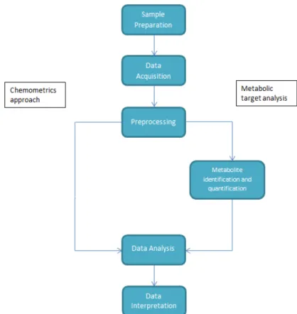
Two distinct approaches can be chosen for planning and executing a metabolomics experiment. The first, known as a chemometrics approach or metabolic fingerprinting, makes use of the preprocessed data, normally spectra or peaks list, and the analysis is done over that data typically for sample discrim-ination. That approach was for instance used in the discrimination between wild and farmed salmon and their origins (Masoum et al.,2007). The second approach, known as metabolic target analysis or profiling focuses on the identification and quantification of compounds present in the sample, being that information used to run the analysis. A metabolic target analysis was for instance used in predict-ing cancer-associated skeletal muscle wastpredict-ing from1H-NMRprofiles of urinary metabolites (Eisner et al.,2010). The second approach is used mostly forNMR data, since identifying and quantifying metabolites inIRandUV-visdata is complex.
The general workflow of a metabolomics experiment generally consists in the steps of sample prepa-ration, data acquisition, preprocessing, data analysis and data interpretation (see Fig. 1). Once the samples are prepared and the data is acquired, it will be preprocessed to correct some issues and im-prove the performance of the next step, data analysis, where the information will be extracted. The last two steps will be the main focus of this project.
Chapter 2.S TAT E O F T H E A R T
Figure 1: General workflow of a metabolomics experiment
2.2.1 Preprocessing
As this step has great importance in the results, almost all the literature has put some thought in preprocessing, testing sometimes a few combinations of methods and analyzing the results obtained, to know which preprocessing methods are better or worse with the data being analyzed. Preprocessing is important to make samples analyzable and comparable. Normally, the preprocessing steps consist on missing values and outlier removal, some peak spectra processing and normalization or scaling.
There are two major choices regarding missing values handling: their removal, removing the feature or the sample containing the missing value, or replacing by a value such as the row or column mean, or using more sophisticated methods (e.g. nearest neighbors). Also, there are sometimes samples or variables that are considered outliers (observation point that is distant from other observations) due to variability in measurement or experimental error. Those are typically excluded from the dataset.
Peak spectra processing refers to corrections or selections made over the spectra. For that task, there are methods such as baseline correction, which, as the names indicates, is needed to correct an unwanted linear or non-linear bias along the spectra. Another method is smoothing, which means reducing the noise of the spectra, and help for both visual interpretation and robustness of the analysis by trying to smooth enough to reduce the noise while retaining as much as possible of the peaks,
2.2. Workflow of a metabolomics experiment
especially the small ones. One popular method of smoothing is the Savitzky-Golay filter which is a process known as convolution that fits successive sub-sets of adjacent data points with a low-degree polynomial by the method of linear least squares.
There are some other methods related to peak spectra processing like binning, peak alignment, among others. Binning is useful when there are a large number of measurements per spectrum, it divides the spectrum into a desired number of bins, forming a new spectra with fewer variables. The reasons for using binning are that the number of variables can be too high and another less obvious reason is the implicit smoothing and the potential for correcting small peak shifts. There are a few dangers regarding the bad placing of the bins, by removing information or producing false informa-tion.
InNMR, peaks can be shifted due to instrumental variations, sample pH or interferences in the anal-ysis, for example. Those shifts need to be corrected before the data analanal-ysis, so that each metabolite appears where it is expected. There are a few methods of doing peak alignment, some simpler than others which are more robust. The simplest form of peak alignment is to divide the spectra into a num-ber of local windows where peaks are shifted to match across spectra. That is fast, since everything is done locally, but may lead to misalignment when peaks fall into the wrong local window or are split into two windows, just as when binning. One of the more robust peak-alignment procedures is called
Correlation Optimized Warping (COW). It uses two parameters – section length and flexibility – to control how spectra can be warped towards a reference spectrum (Liland,2011).
In many cases, to make variables comparison possible, the data needs to be standardized to be comparable. The common process of standardizing values does their subtraction by the mean and division by the standard deviation. An alternative process is the use of median and the mean absolute deviation. Centering the data can make many data analysis techniques work better and it means that the mean spectrum is subtracted from each of the spectra. It depends on the particular dataset whether centering the data does make sense or not.
The calculation of derivatives of the spectrum is often used mostly inUV-visandIRspectroscopy. It is the result of applying a derivative transform to the data of the original spectrum, being useful for two reasons: the first and second derivatives may swing with greater amplitude then the original spectra, in many cases separating out peaks of overlapping bands. In some cases, this can be a good noise filter since changes in baseline have negligible effect on derivatives. Multiplicative Scatter Correction (MSC) is a pre-processing step needed for measurement of many elements. It is a transformation method used to compensate for additive and/or multiplicative effects in spectral data.
On ultraviolet-visible spectroscopy’s metabolomics literature, it can be perceived that in compar-ison to infrared spectroscopy, less methods were used regarding peak spectra processing and the raw data were typically just normalized and derivatives calculated (check Table 1). On infrared spectroscopy, more methods for peak spectra processing were applied such as smoothing, with the Savitzky-Golay method being the most used, baseline and scatter correction, most often usingMSC. In this case, derivatives were also calculated (first and second derivatives) and the data normalized.
Chapter 2.S TAT E O F T H E A R T
OnNMRdata, peak spectra processing was employed such as peak alignment, binning and baseline correction, while usually standardization is also applied.
The methods of preprocessing used can vary much from dataset to dataset, taking into account the data’s quality and the type of the data. In Table1, the various preprocessing methods used in several cases from the literature are summarized in the fourth column.
2.2.2 Metabolite identification and quantification
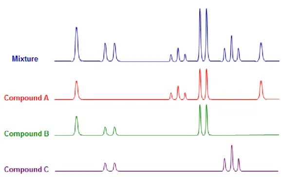
SinceNMRproduces a large number of peaks from possibly hundreds of metabolites, the identifica-tion and quantificaidentifica-tion of metabolites is quite difficult due to shifting peak posiidentifica-tions, peak overlap, noise and effects of the biological matrix. Figure2 shows an example of peak overlap. So, this is a complex problem to solve with 100% accuracy, but there are some tools that achieve good results such asBayesian AuTomated Metabolite Analyser for NMR spectra (BATMAN), MetaboMiner or Metabohunter which will be described briefly next.
BATMAN, is an R package which deconvolutes peaks from 1-dimensionalNMRspectra, automat-ically assigning them to specific metabolites and obtaining concentration estimates. The Bayesian model incorporates information on characteristic peak patterns of metabolites and is able to account for shifts in the position of peaks commonly seen inNMR spectra of biological samples. It applies aMarkov Chain Monte Carlo (MCMC)algorithm to sample from a joint posterior distribution of the model parameters and obtains concentration estimates with reduced mean estimation error compared with conventional numerical integration methods (Hao et al.,2012).
MetaboMiner is a standalone graphics software tool which can be used to automatically or semi-automatically identify metabolites in complex biofluids from 2DNMRspectra. MetaboMiner is able to handle both 11H-1H Total Correlation Spectroscopy (TOCSY) and1H-13C heteronuclear single quantum correlation (HSQC) data. It identifies compounds by comparing 2D spectral patterns in theNMRspectrum of the biofluid mixture with specially constructed libraries containing reference spectra of 500 pure compounds. Tests using a variety of synthetic and real spectra of compound mixtures showed that MetaboMiner is able to identify >80% of detectable metabolites from good qualityNMRspectra (Xia et al.,2008).
MetaboHunter is a web server application which can be used for the automatic assignment of1
H-NMRspectra of metabolites. MetaboHunter provides methods for automatic metabolite identification based on spectra or peak lists with three different search methods and with the possibility for peak drift in a user defined spectral range. The assignment is performed using as reference libraries manually curated data from two major publicly available databases ofNMRmetabolite standard measurements (HMDB and MMCD). Tests using a variety of synthetic and experimental spectra of single and multi-metabolite mixtures have shown that MetaboHunter is able to identify, in average, more than 80% of detectable metabolites from spectra of synthetic mixtures and more than 50% from spectra corre-sponding to experimental mixtures (Tulpan et al.,2011).
2.2. Workflow of a metabolomics experiment
Figure 2: Example of a peak overlap
2.2.3 Univariate data analysis
On data analysis, the input is usually a matrix, with either a compound list or a peak list and their values for different samples. Either way, the complexity of metabolomics data requires complex analysis methods. Data analysis can be used to predict values like beer quality parameters (Polshin et al.,2011) or to predict the class label of a certain sample, as in the identification of the farm origin of salmon (Martinez et al.,2009). There are three main types of methods for data analysis: univariate analysis, unsupervised multivariate techniques and supervised multivariate techniques, these last two explained in more detail insubsection 2.2.4andsubsection 2.2.5. With the first approach, the analysis is carried out on a single variable at a time and several statistical measures can be employed to describe the data. The unsupervised and supervised multivariate approaches on the other hand use more than one statistical outcome variable at a time in the analysis. The differences between the last two is that the first do not use any metadata, e.g. information about natural groups within the data, while the latter requires samples that are divided into at least two classes (or groups) to allow the methods to conduct a learning (or training) process.
This section will focus on univariate statistical analysis. From the many techniques, a few most popular ones will be explained given their importance in metabolomics data analysis, namely t-tests,
Analysis of Variance (ANOVA)and fold change analysis.
A t-test is a statistical hypothesis test in which the test statistic follows a Student’s t distribution.It can be used only for situations where the data is splitted into two groups, being applied to a single data variable. The method can determine if the means of the variable in the two groups are significantly
Chapter 2.S TAT E O F T H E A R T
different from each other by giving a p-value. If this value is inferior to 0.05 (or any other significance level that is selected) the null hypothesis is rejected, which means that we can say that the means of the variable for the two groups are different. On the contrary, if the p-value is superior to 0.05, the null hypothesis cannot be rejected, which means that the estimate of the mean of the two groups can be identical. Applied to metabolomics, t-tests can be used on each of the variables (ppm, wavelength, etc) to see what are the most significant ones in the discrimination between two classes.
ANOVAconstitutes a set of statistic models and tests associated that is used to analyze the differ-ences between group means and associated procedures. In the simplest form ofANOVA, one-way
ANOVA, it provides a statistical test to check if the means of several groups are equal, and so it gen-eralizes the t-test to more than two groups. Some post hoc tests can be used withANOVA like the Tukey’sHonest Significance Difference (HSD)test used to compare all possible pairs of group means. The F-test plays an important role in one-wayANOVA, it is used for testing the statistical signif-icance by comparing theF statistic, which compares the variance between groups with the variance within groups. The ANOVAF-test is known to be nearly optimal in the sense of minimizing false negative errors for a fixed rate of false positive errors.
In the cases where multiple tests need to be conducted, as it is the case with metabolomics data, the p-values can be adjusted for multiple testing using various methods. One of the most common is theFalse Discovery Rate (FDR). It controls the expected proportion of false discoveries amongst the rejected hypotheses. TheFDRis a less stringent condition than the family-wise error rate.
AnANOVAonly tells you that there are differences between your groups, not where they lie. There-fore a post-hoc test like Tukey’sHSDcan be used to examine where the differences lie.
Also,ANOVAgeneralizes to the study of the effects of multiple factors (Two-wayANOVA, three-wayANOVA, etc). It examines the influence of two or more different categorical independent vari-ables on one dependent variable. It can determine the main effect of contributions of each independent variable and also identifies if there is a significant interaction effect between them .
The Fold Change (FC) is a measure that shows how much a variable mean changes within two groups. It is calculated by getting the ratio of the mean value of the variable in one group to the same value in the other group. The higher the fold change value is for a feature, the more likely that feature is significant to discriminate the two groups.
2.2.4 Unsupervised Methods
Usually,Principal Component Analysis (PCA)is employed to check if natural groups (clusters) arise and/or to reduce dimensionality. PCAis the most frequently applied method for computing linear latent variables (components). PCAcan be seen as a method to compute a new coordinate system formed by the latent variables (which are orthogonal) and where only the most informative dimensions are used. Latent variables fromPCAoptimally represent the distances between the objects in a high-dimensional variable space. It is a very popular technique and it is used frequently on all types
2.2. Workflow of a metabolomics experiment
of metabolomics data (Varmuza and Filzmoser, 2008). The results of a PCA analysis include the scores of the supplied data on the principal components, i.e. the transformed variable values that corresponds to a particular data point, the matrix of variable loadings, which are the weights of each original variable on the new coordinates and the standard deviations (or variance) explained by each of the principal components (or cumulative).
Also, to verify if natural groups arise and determine their composition, clustering techniques such as k-means or hierarchical clustering can be used. Cluster analysis tries to identify coherent groups (i.e., clusters) of objects, while no information about any group membership is available, and usually not even the optimal number of clusters is known. In other words, cluster analysis tries to find groups containing similar objects (Varmuza and Filzmoser,2008). There are two main types of clustering methods, hierarchical and nonhierarchical clustering.
Hierarchical Cluster Analysis (HCA)organizes data in tree structures with the main clusters con-taining subclusters and so on. Generally, there are two types ofHCA, the first is agglomerative which means that the process starts with each observation as a cluster, and then pairs of clusters are merged as the hierarchy moves up. On the other hand, the second approach is divisive, which means that all observations start in a single cluster and then the splits are done recursively as the hierarchy moves down. The result from HCAis generally a dendrogram. In order to know what clusters should be splitted or merged, a measure of dissimilarity between sets of observations is required. Commonly that measure is achieved with the use of a distance metric between two observations (e.g. Euclidean or Manhattan distances) and a linkage criterion (e.g. nearest neighbour or complete linkage) that calculates the distance between sets of observations as a function of the pairwise distances between observations.
Nonhierarchical clustering organizes data objects into a set of flat groups (typically non overlap-ping). It is a class of methods that aim to partition a dataset into a pre-defined number of clusters, typically using iterative algorithms that optimize a chosen criterion. One important methods is k-means clustering, where heuristics that start from initial random clusters, proceeds by transferring observations from one cluster to another, until no improvement in the objective function can be made. k-means clustering is a nonhierarchical clustering method that seeks to assign each observation to a cluster, minimizing the distance of the observation to the cluster mean.
2.2.5 Supervised Methods: machine learning
The general workflow of machine learning consists of creating predictive models in order to classify new samples to a specific output, i.e. the goal is to learn a general rule that maps the inputs into outputs. To construct a predictive model, the learner algorithm must generalize from its experience, i.e. training examples must be provided (labeled) and from those, the learner has to build a general model to try to predict new unlabeled samples with good accuracy results. There are two approaches, classification and regression. Classification is used when the output that we are trying to predict is a
Chapter 2.S TAT E O F T H E A R T
non-numeric value, i.e. a set of categories, and the algorithm will try to assign the unlabeled sample to one of the categories. Regression is used when the output is a numeric value and the algorithm will try to predict the numeric output value for the new sample.
Besides the accuracy, which is the proportion of samples correctly classified, to evaluate the per-formance of the models built, there are many other metrics, like the Kappa statistic, which compares the observed accuracy with an expected accuracy. The calculation of the expected accuracy is related to the actual number of instances of each class, along with the number of instances that the classifier labeled for each class. Letnc be the number of classes, tibe the actual number of instances of a class i, cithe number of instances that the classifier labeled as belonging to that class andn the total number of instances, the expected accuracy is calculated as it shows in Equation1.
expected_accuracy= nc ∑ i=1 ti×ci n n (1)
Formula 1: Expected accuracy
Now the Kappa statistic can be calculated using both the observed accuracy and the expected accu-racy, as shown in Formula2.
kappa_statistic= observed_accuracy−expected_accuracy
1−expected_accuracy (2)
Formula 2: Kappa statistic
Essentially, the Kappa statistic is a measure of how closely the instances classified by the classifier matched the actual data label, controlling for the accuracy of a random classifier as measured by the expected accuracy.
Popular supervised methods, used commonly in metabolomics experiments, arePartial Least Squares - Discriminant Analysis (PLS-DA)(Partial least squares – discriminant analysis), k-Nearest
Neigh-bors (kNN),Linear Discriminant Analysis (LDA)andSoft Independent Modeling of Class Analogy (SIMCA)for classification tasks. For regression,Partial Least Squares - regression (PLS-r)(Partial least squares – regression) is usually applied.
Partial Least Squares (PLS)is a supervised multivariate calibration technique that aims to define the relationship between a set of predictor data X (independent variables) and a set of responses Y(dependent variables). The PLS method projects the initial input–output data down into a latent space, extracting a number of principal components, also known as Latent Variables (LV) with an orthogonal structure, while capturing most of the variance in the original data. The firstLVconveys the largest amount of information, followed by the secondLVand so forth.PLS-DAis a variant used when the Y is categorical (Varmuza and Filzmoser,2008).
2.2. Workflow of a metabolomics experiment SIMCAis a method based on disjoint principal component models proposed by Svante Wold. The idea is to describe the multivariate data structure of each group separately in a reduced space using
PCA. The special feature of SIMCAis that PCAis applied to each group separately and also the number of PCs is selected individually and not jointly for all groups. A PCAmodel is an envelope, in the form of a sphere, ellipsoid, cylinder, or rectangular box optimally enclosing a group of objects. This allows for an optimal dimension reduction in each group to reliably classify new objects. Due to the use ofPCA, this approach works even for high-dimensional data with a small number of samples. In addition to the group assignment for new objects, SIMCA also provides information about the relevance of different variables to the classification or measures of separation (Varmuza and Filzmoser,
2008).
K-nearest neighbor (kNN) classification methods require no model to be fitted because they can be considered as memory based. These methods work in a local neighborhood around a considered test data point to be classified. The neighborhood is usually determined by the Euclidean distance, and the closest k objects are used for estimation of the group membership of a new object.
Also, more sophisticated machine learning techniques have been used to build classification models in order to give good prediction results. Techniques likeArtificial Neural Network (ANN),Support Vector Machine (SVM)s (Support Vector Machines), random forests, decision trees and rule induction algorithms were applied on some metabolomics experiments with very good results onNMR,IRand
UV-visdata that can be used to predict new unlabeled samples (see Table1).
SVMs are a machine learning approach that can be used for both classification and regression. In the context of classification they produce linear boundaries between object groups in a transformed space of the variables (using a kernel), which is usually of much higher dimension than the original space. The idea of the transformed higher dimensional space is to make groups linearly separable. Furthermore, in the transformed space, the class boundaries are constructed to maximize the margin between the groups. On the other hand, the back-transformed boundaries are nonlinear.
Decision trees are represented by n-ary trees where each node specifies a test to the value of a certain input attribute and each branch that exits the node corresponds to a value of that attribute, originating a similar sub-tree. In the bottom of the tree are the leaves that represent the predicted values. The classification process is recursive, beginning in the root of the tree and going from branch to branch according to the attribute value until a leaf is reached. An example of this technique is the C4.5 algorithm and its implementation in the J48 method included in the WEKA data mining tool (Quinlan,1993;Witten et al.,2011).
Classification rules follow a similar structure as decision trees, but instead of an n-ary tree, they consist of a list of rules ordered by the quality of the rules. If an example’s attributes follow the con-ditions of the rules then the classification output is the output value of the rule. An implementation of this is JRip, which implements a propositional rule learner,Repeated Incremental Pruning to Produce Error Reduction (RIPPER)(Cohen,1995;Witten et al.,2011).
Chapter 2.S TAT E O F T H E A R T
Random forests are an ensemble learning method for classification and regression, consisting of a set of decision trees. It uses the bagging method as a way to choose the examples and selects the set of attributes to test in each tree randomly. The CART algorithm is used as the tree induction algorithm and uses the out-of-bag error for validation (Breiman,2001).
ANNare computational representations that mimic the human brain, trying to simulate its learning process. The term "artificial" means that neural nets are implemented in computer programs that are able to handle the large number of necessary calculations during the learning process. The most popular type ofANN has three layers, the input layer, the hidden layer and the output layer. Input data are put into the first layer, the hidden layer nodes do some calculations and the output is gathered from the last layer.ANNs can be used for regression and classification.
In Table1, some of these (and other) methods used in metabolomics data analysis studies available in the literature are listed. These include tasks of visual analysis, data reduction, classification and regression tasks.
2.2.6 Feature Selection
Feature selection tries to find the minimum set of features (in metabolomics, can be compounds or peaks, for instance) that achieves maximum prediction performance. Feature selection is important in various ways. It makes models more robust and generally improves accuracy, also providing im-portant information to users regarding which variables are more discriminant. There are two main approaches: filters and wrappers. Filters select features on the basis of statistical properties of the val-ues of the feature and those of the target class, while wrappers rely on running a particular classifier and searching in the space of feature subsets, based on an optimization approach.
A number of feature selection methods has been proposed in the literature. Among them, the most popular wrappers are interval selection methods, such asinterval Partial Least Squares (iPLS)used in species identification using infrared spectroscopy (Lima et al.,2011) andGenetic Algorithms (GA)
used in bacteria discrimination usingFTIRspectroscopy (Preisner et al.,2007).
In theiPLSmethod, the data are subdivided into non-overlapping partitions; each of these groups undergoes a separatePLS modeling to determine the most useful variable set. To capture relevant variation in the output, models based upon the various intervals usually need a different number of
PLScomponents than do full-spectrum models (Balabin and Smirnov,2011).
AGAis a metaheuristic optimization algorithm that has a population of candidate solutions. Over a number of generations, it will evolve the population of candidate solutions, generating new solutions in each generation using selection operators and reproduction operators. For each solution its quality is given by a fitness value, calculated using a defined objective function.
Also Recursive Feature Elimination (RFE), also known as backward selection, is a wrapper ap-proach. It first uses all features to fit the model, and then each feature is ranked according to its importance to the model. Then for each subset the most important variables are kept and the model
2.3. Databases of metabolomics data
is refitted and performance calculated, with the rankings for each feature recalculated. Finally, the subset with the best performance is determined and the top features of the subset are used to fit the final model.
Regarding filter approaches, simple univariate statistical tests can be used to pre-select the features that pass some specific criterion (e,g. information gain, correlation with output variable) and then the model is built with those selected features. Also flat pattern filters that remove variables with low variability among instances can be used to filter the features prior to the construction of the model.
2.3 D ATA B A S E S O F M E TA B O L O M I C S D ATA
As said before, the number of databases of metabolomics data made available to the public is growing (Table 2). The most notable database that can be mentioned is the Human Metabolome Database (http://www.hmdb.ca/). For experimental data, there is also MetaboLights (http://www. ebi.ac.uk/metabolights/). Other databases provide also complementary information about metabolites and metabolism, such as KEGG (http://www.genome.jp/kegg/), PubChem (http:
//pubchem.ncbi.nlm.nih.gov/) and others.
2.3.1 HMDB
The Human Metabolome Database is a freely available electronic database containing detailed infor-mation about small molecules (metabolites) found in the human body. It is intended to be used for ap-plications in metabolomics, clinical chemistry, biomarker discovery and general education. Four addi-tional databases, DrugBank (http://www.drugbank.ca), T3DB (http://www.t3db.org), SMPDB (http://www.smpdb.ca) and FooDB (http://www.foodb.ca) are also part of the HMDB suite of databases. DrugBank contains equivalent information on ∼1600 drugs and drug metabolites, T3DB contains information on 3100 common toxins and environmental pollutants, and SMPDB contains pathway diagrams for 440 human metabolic and disease pathways, while FoodDB contains equivalent information on ∼28,000 food components and food additives. (Wishart et al.,
2013)
2.3.2 MetaboLights
MetaboLights is a database for metabolomics experiments and derived information. The database is cross-species, cross-technique and covers metabolite structures and their reference spectra as well as their biological roles, locations and concentrations, and experimental data from metabolic experi-ments. It will provide search services around spectral similarities and chemical structures (Haug et al.,
Chapter 2.S TAT E O F T H E A R T
Name URL Short description
HMDB http://www.hmdb.ca Detailed information on metabolites found in the human body Metabolights http://www.ebi.ac.uk/metabolights Database for metabolomics experiments and derived information
MMMDB http://mmmdb.iab.keio.ac.jp Mouse multiple tissue metabolome database SMDB http://www.serummetabolome.ca Serum metabolome database
MeKO@PRIMe http://prime.psc.riken.jp/meko/ A web-portal for visualizing metabolomic data of Arabdiopsis MPMR http://metnetdb.org/mpmr_public/ A metabolome database for medicinal plants
ECMDB http://www.ecmdb.ca/ E. coli metabolome database YMDB www.ymdb.ca Yeast metabolome database SMPDB http://www.smpdb.ca Small Molecule Pathway Database
FooDB http://www.foodb.ca Resource on food constituents, chemistry and biology DrugBank http://www.drugbank.ca Combines drug data with comprehensive drug targets
BMRB http://www.bmrb.wisc.edu/metabolomics Central repository for experimentalNMRspectral data MMCD http://mmcd.nmrfam.wisc.edu Database on small molecules of biological interest BML-NMR http://www.bml-nmr.org/ Birmingham Metabolite LibraryNMRdatabase
IIMDB http://metabolomics.pharm.uconn.edu/iimdb Both known and computationally generated compounds KEGG http://www.genome.jp/kegg/ Contains metabolic pathways from a wide variety of organisms PubChem http://pubchem.ncbi.nlm.nih.gov Database of chemical structures of small organic molecules
Table 2: Databases of metabolomics data
2.4 AVA I L A B L E F R E E T O O L S F O R M E TA B O L O M I C S
Computational tools for metabolomics have been growing in the past years being already available a good set of free tools (Table3). One notable example is MetaboAnalyst (Xia et al., 2009,2012), a web-based metabolomic data processing tool. It accepts a variety of input data (NMRpeak lists, binned spectra,Mass Spectrometry (MS)peak lists, compound/concentration data) in a wide variety of formats. It also offers a number of options for metabolomic data processing, data normalization, multivariate statistical analysis, visualization, metabolite identification and pathway mapping. In par-ticular, MetaboAnalyst supports methods such as: fold change analysis, t-tests,PCA,PLS-DA, hier-archical clusteringSVMs. It also employs a large library of reference spectra to facilitate compound identification from most kinds of input spectra. It works based on the open-source R scientific com-puting platform (http://www.r-project.org).
Also, there are several packages from Bioconductor project (http://www.bioconductor. org) for R, which target a set of biological data analysis tasks, focusing on omics data, with some specific metabolomics packages mainly forMS, which is another technique for metabolomics data ac-quisition that will not be the focus here (http://bioconductor.org/packages/release/
BiocViews.html#___Metabolomics).
Still for R, there two important packages, hyperSpec and ChemoSpec. ChemoSpec is a collection of functions for plotting spectra (NMR,IR, etc) and carrying out various forms of top-down exploratory data analysis, such asHCA,PCAand model-based clustering. Robust methods appropriate for this type of high-dimensional data are employed. ChemoSpec is designed to facilitate comparison of samples from treatment and control groups. It also has a number of data pre-processing options available, such as normalization, binning, identifying and removing problematic samples, baseline correction, identifying and removing regions of no interest like the water peak in1-NMRor theCO2 peak inIR(Hanson,2013).
2.5. Data integration
Name URL Short description
MetaboAnalyst http://www.metaboanalyst.ca Web application to analyze metabolomic data hyperSpec http://hyperspec.r-forge.r-project.org R package to handle spectral data and metadata ChemoSpec http://cran.r-project.org/web/packages/ChemoSpec R package to handle spectral data
Metabolomic Package http://cran.open-source-solution.org/web/packages/Metabonomic/ R-package GUI for the analysis of metabonomic profiles
speaq https://code.google.com/p/speaq/ Integrated workflow for robust alignment and quantitative analysis ofNMR
Automics https://code.google.com/p/automics/ Platform forNMR-based spectral processing and data analysis
MeltDB https://meltdb.cebitec.uni-bielefeld.de Web-based system for data analysis and management of metabolomics
metabolomics http://cran.r-project.org/web/packages/metabolomics Collection of functions for statistical analysis of metabolomic data
metaP-Server http://metabolomics.helmholtz-muenchen.de/metap2/ Web application to analyze metabolomic data Bioconductor http://bioconductor.org/packages/release/BiocViews.html
#___Metabolomics Bioconductor R packages for metabolomics
Table 3: Available free tools for metabolomics data
hyperSpecis a R package that allows convenient handling of hyperSpectral data sets, i. e. data sets combining spectra with further data (metadata) on a per-spectrum basis. The spectra can be anything that is recorded over a common discretized axis. hyperSpec provides a variety of possibilities to plot spectra, spectral maps, the spectra matrix, etc. It also provides preprocessing and data analysis methods. Regarding proprocessing, hyperSpec offers a large variety of methods, such as cutting the spectral range, shifting spectra, removing bad data, smoothing, baseline correction, normalization or
MSC. In data analysis,PCAand clustering techniques can be performed with this package (Beleites,
2012).
As wee can see from Table3, there are many tools for the metabolomics analysis, but MetaboAna-lyst, which is the only integrated framework looses flexibility because it is more oriented to graphical user interfaces (GUI).
2.5 D ATA I N T E G R AT I O N
Data integration tries to aggregate data from different techniques in order to improve performance of the prediction models; this is also known as data fusion. There are mainly three types of fusion strategies, namely, information/data fusion (Low-Level Fusion (LLF)), feature fusion ( Intermediate-Level Fusion (ILF)), and decision fusion (High-Level Fusion (HLF)). The first two work on variable level while the latter works on the decision level.
Variable level integration concatenates the variables into a single vector, which is called a “meta-spectrum”. Data must be balanced (all variables in the same scale) prior to the fusion process. If the number of concatenated variables is quite high, a variable selection is required. LLF involves combining the outputs from two or more techniques to create a single signal (see Fig. 3). ILFfirst involves feature extraction onto each source of data, followed by a simple concatenation of the feature sets obtained from multiple information sources (see Fig. 4) (Subari et al., 2012). Decision level
Chapter 2.S TAT E O F T H E A R T
data fusion combines the classification results obtained from each individual technique using different methods like fuzzy set theory or Bayesian inference.
There are some studies using data integration from different techniques. In some, data integration does not improve classification performance significantly comparing to the individual results, but in some other cases, data integration can improve significantly the classification results.
Data fusion for determining Sudan dyes in culinary spices (Anibal et al.,2011), which combines data from1H-NMRandUV-visspectroscopy, applies the two types of data integration and uses fuzzy set theory in the decision level approach, improving the overall performance of classification. Also pure and adulterated honey classification (Subari et al.,2012), which combines data from e-nose and
IRspectroscopy, two types of variable level data integration, namelyLLFandILF, gave better results than a single technique alone.
Classifying white grape musts in variety categories (Roussel et al.,2003a,b), which combines data fromUV-visandIRspectroscopy, also applies the two main approaches. The variable level approach,
LLF, does not significantly improve results while the decision level approach, which employs data integration based on the Bayesian inference, improved the classification results.
Figure 3: Low-level fusion example
Figure 4: Intermediate-level fusion example
3
D E V E L O P M E N T
This chapter will cover the details about the developed package and the development process. The general structure to keep spectral or other types of metabolomics data will be explained, as well as the different functional sections of the package such as: the preprocessing, univariate analysis, unsupervised and supervised multivariate analysis, including machine learning and feature selection. Also, the technologies used (software, plugins, packages, etc) will also be referenced.
3.1 D E V E L O P M E N T S T R AT E G Y A N D T O O L S
To achieve the defined goals, a package with features covering the main steps of the metabolomics data analysis workflow was developed, containing functions for the data reading and dataset creating, preprocessing and data analysis.
The package was developed with functions easy to call, i.e. with few mandatory parameters, but also very flexible, since while most functions have default parameters, they also have a large number of parameters that users can use to change the default behavior. The package integrates many functions imported and sometimes adapted from other packages, integrating various packages over a unique interface. The package’s functions were meant to be easy to use and to provide abundant graphical visualization options of the results. The idea is to minimize the number and complexity of the lines of code needed to make a pipeline analysis over a certain dataset, but also to easily allow creating variants for this analysis with low complexity.
The package was developed using the R environment (http://www.r-project.org), a free integrated software environment for data manipulation, scientific and statistical computing and graph-ical visualization. The most relevant characteristics of this platform are the data handling and storage facilities, a base set of operators for matrix calculations, a large set of tools for data analysis, the graphical facilities that can generate various types of graphics for data analysis. Also, it has a well developed and effective programming language, the ’S’ language, allowing to develop new functions and scripts. Since it is a free environment, it has the contribution of a large collection of packages developed by anyone who wants to contribute (Venables et al.,2014). With such characteristics and the goal of this thesis in mind, the choice of using R became clear.