UNIVERSIDADE DE LISBOA
INSTITUTO SUPERIOR DE ECONOMIA E GESTÃO
MESTRADO EM ECONOMIA MONETÁRIA E
FINANCEIRA
T
RABALHO
F
INAL DE
M
ESTRADO
D
ISSERTAÇÃO
T
HE
I
MPACT OF THE
Q
UANTITATIVE
E
ASING
P
ROGRAMS ON THE
N
ORTH
A
MERICAN
E
QUITY
M
ARKET
ALUNO:
F
RANCISCO
N
UNES
M
OUTINHO
S
ALGADO
R
UANO
UNIVERSIDADE DE LISBOA
INSTITUTO SUPERIOR DE ECONOMIA E GESTÃO
MESTRADO EM ECONOMIA MONETÁRIA E
FINANCEIRA
T
RABALHO
F
INAL DE
M
ESTRADO
D
ISSERTAÇÃO
T
HE
I
MPACT OF THE
Q
UANTITATIVE
E
ASING
P
ROGRAMS ON THE
N
ORTH
A
MERICAN
E
QUITY
M
ARKET
ALUNO:
F
RANCISCO
N
UNES
M
OUTINHO
S
ALGADO
R
UANO
O
RIENTAÇÃO:
J
ORGEM
ANUEL DEA
ZEVEDOH
ENRIQUES DOSS
ANTOSI
Agradecimentos
Em primeiro lugar, gostaria de agradecer ao Professor Jorge Henriques dos Santos pela sua disponibilidade, sugestões e conhecimento transmitido ao longo da elaboração desta dissertação, bem como ao longo das aulas de Macroeconomia no Mestrado de
Economia Monetária e Financeira.
Se é um facto que apenas do trabalho árduo provém o sucesso e a realização pessoal, gostaria de agradecer a todos os professores do Mestrado de Economia Monetária e Financeira, do Instituto Superior de Economia e Gestão, pelo nível de dedicação, trabalho e esforço exigido ao longo destes dois anos.
Por último, mas não menos importante, gostaria de agradecer a todos os amigos que me acompanharam ao longo dos anos de percurso académico e pessoal, bem como à minha família que sempre me apoiou, com um especial agradecimento para a minha mãe e a minha irmã.
II
Abstract
The aim of this research is to assess how the unconventional monetary policy instruments used by the Federal Reserve impacted on the North American Stock Market from the period between January 2009 and September 2012.
We present the economic theory concerning the transmission mechanism of the monetary policy to the Economy, the channels through which this transmission becomes effective and, in particular, the functioning of the stock price transmission channel. We also present the economic theory on how unconventional monetary policy instruments, the Quantitative Easing programs, impact on assets and particularly on the stock prices. In the spirit of the Arbitrage Pricing Theory (APT) we develop a GARCH model in order to assess which macroeconomic, financial and conventional and unconventional monetary variables impacted on the evolution of the North-American Stock market in the period referred above.
We observe that almost all of the variables chosen in this study tend to impact on the equity prices in the long run, but they have no impact in a period of financial distress such as the one between January 2009 and September 2012. We also found no evidence that the Quantitative Easing programs launched by the Federal Reserve after January 2009 had a permanent and direct impact on the recovery of the North American Markets until September 2012.
Keywords: Quantitative Easing, Monetary Policy, Stock Market, FED JEL Classification: E52, E44, E58
III
Resumo
O presente trabalho tem como objectivo avaliar se a política monetária não
convencional, levada a cabo pela Reserva Federal Norte-Americana (FED) entre Janeiro de 2009 e Setembro de 2012, teve impacto na recuperação do Mercado Accionista dos Estados Unidos da América no referido período.
Em primeiro lugar, começamos por apresentar a teoria económica referente à transmissão da política monetária para os restantes agregados macroeconómicos, os canais através dos quais essa transmissão se processa e, em particular, através do canal do mercado accionista. Apresentamos, também, a teoria relativa ao modo como os programas de Quantitative Easing afectam os diversos activos financeiros e, em especial, a evolução do mercado accionista.
Em seguida, e no espírito da Arbitrage Pricing Theory (APT), desenvolvemos um modelo GARCH que nos permite avaliar quais as variáveis macroeconómicas,
financeiras e de política monetária convencional e não convencional, que influenciaram a evolução do mercado accionista norte-americano no período supra referido.
Verificamos que a quase totalidade das variáveis consideradas têm um impacto estatisticamente significativo no mercado accionista quando consideramos períodos temporais longos, mas aparentam não ter impacto em períodos de instabilidade financeira, como os vividos entre Janeiro de 2009 e Setembro de 2012. De referir, também, que não encontramos evidência empírica de que os programas de Quantitative Easing, lançados pela FED após Janeiro de 2009, tivessem tido um impacto directo e permanente na recuperação do mercado accionista norte-americano.
Palavras-Chave: Política Monetária Não-Convencional, Mercado Accionista, Reserva
IV
Index
Agradecimentos ... II
Abstract ... II
Resumo ... III
Index ... IIIV
1.
Introduction ... 1
2.
The Monetary Policy and The Stock Price Transmission Channel . 5
3.
The Impact of the QE Programs on US Equity Market: An
Empirical Assessment ... 16
3.1. Empirical Assessment Rationale ... 17
3.2. Explanatory Variables ... 18 3.3. Series ... 20 3.4. Methodology ... 23 3.5. Empirical Results ... 26
4.
Conclusions ... 34
5.
References ... 38
1
1. Introduction
In the United States of America, the beginning of the Subprime Crisis in the summer of 2007 had a substantial impact on all segments of the financial markets.
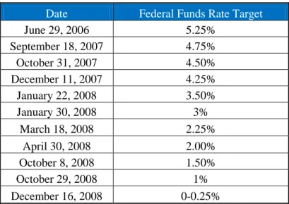
The North-American equity market index, S&P500, fell from a historical maximum at that time of 1553.08 points, on July 19, to 1406.7 points on August 15,with investors fearing the impact of the crisis on the future cash-flows of American companies. The Federal Reserve (FED) started to cut the official interest discount rate1 and the target for the federal funds rate2 the first time in September 2007, from 5.25% to 4.75%. After this first cut in the target for the federal funds rates, the FED reduced this target progressively during the following year until it reached the range of 0 to 0.25%, on December 162008.
Date Federal Funds Rate Target
June 29, 2006 5.25% September 18, 2007 4.75% October 31, 2007 4.50% December 11, 2007 4.25% January 22, 2008 3.50% January 30, 2008 3% March 18, 2008 2.25% April 30, 2008 2.00% October 8, 2008 1.50% October 29, 2008 1% December 16, 2008 0-0.25%
Table I: Federal Funds Rates Target. Source: Federal Reserve Bank of New York
1
The interest rate charged to commercial banks and other depository institutions on loans they receive from their regional Federal Reserve Bank's lending facility.
2 The interest rate at which depository institutions lend reserve balances to other depository institutions
2 At this point, the US Economy faced the Zero Lower Bound meaning that the FED had no longer available the main instrument of monetary policy, the discount rate and its direct influence over the very short-term interest rate. North-American equity markets did not start to recover during this period which can be easily perceived in figure 1.
Figure 1: S&P500 value from April, 2007 to January, 2009. Source: Yahoo Finance
In aggregate terms, from July 19, 2007 to the end of December 2008, S&P 500 had a devaluation of 41.8%.
In this particular period the aggressive cuts in the FED official rates seemed to have little impact on the US stock prices. Although the 3 month treasury bill rate which is often used as a proxy for the risk-free rate, had dropped from 4.96% in July 2007 to 0.11% in December 2008, the lack of investors’ confidence in future economic conditions did not lead them to increase the demand for more risky assets like stocks . The State Street Investors Confidence Index measuring the willingness of investors to hold risky assets like equity, dropped from 108.5 in June 2007 to 82.8 points in December 2008, and the VIX index that measures the volatility in the market rose from
3 23.52 in July 2007 to 40 points in December 2008, showing the particular apprehension that was being felt by investors in the equity market at that time.
Conventional monetary tools were not being totally effective in promoting a sustainable US economic recovery and restoring confidence in financial markets (Bernanke, 2009) and consequently on November 25, 2008, the FED announced that it would start a Large Scale Asset Purchases (LSAP) program in order to enhance the credit markets’ conditions. This program, also known as a Quantitative Easing (QE) program, consisted of a large scale purchase of long-term Treasury Bonds, Agency Debt and Agency Mortgages Backed Securities (MBS) to an extent of $1.75 trillion in the three types of assets, allowing the increase of the FED’s Balance Sheet. This marks the post subprime crisis first utilization of unconventional monetary tools by the FED in a non-pure quantitative easing policy because “ […] in a pure QE regime, the focus of policy is the quantity of bank reserves, which are liabilities of the central bank; the composition of loans and securities on the asset side of the central bank’s balance sheet is incidental […] In contrast, the Federal Reserve’s credit easing approach focuses on the mix of loans and securities that it holds and on how this composition of assets affects credit conditions for households and businesses” (Bernanke, 2009).
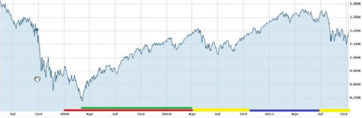
When the QE program was officially launched on December 16, 2008 the S&P 500 had a value of 913.18 points and by the end of this first QE program on March 31, 2010 its value was 1169.43, representing an increase of 22% (red line period in figure 2). Since the end of March 2010 until the new FED’s announcement of a second LSAP program, the S&P500 remained almost in the same value just having an increase from 1178.1 on April 1, 2010 to 1183.26 on November 1, 2010 which represents an increase of only 0.43% (first yellow line period in figure 2). During the second QE program the S&P500
4 rose from 1183.26 on November 1, 2010 to 1307.41 on June 29th 2011 representing an increase of 10.5% in its value (blue line period in figure 2).
As we can observe in figure 2, during the periods when the QE programs I and II were active, the S&P500 increased substantially. However, when the FED’s large scale purchases were suspended, the S&P500 value decreased or simply remained stable.
Figure 2: S&P500 from May 2008 to October, 2011. Source: Yahoo Finance and the Author
When the QE I was announced on November 25, 2008 the S&P500 rose 1% in that trading session and 3.4% in the following day. Between November 25 and November 28 the S&P500 rose 5.2% in aggregate terms. Two years after, when QE II was announced on November 3, 2010 S&P500 rose 1.15% on that day’s trading session, 2% on the following day and 0.4% on November 5. In aggregate terms S&P 500 rose 3.5% in the two days after the second QE announcement. These increases in S&P 500 seem to show that the pursuing of a large asset purchasing policy was well perceived by the investors.
This dissertation will measure the possible impact of the Federal Reserve’s Large Scale Asset Purchases on the North-American Equity Markets. This analysis is important not only for monetary policy but also for financial investment purposes. In the first place, it
5 is important for a Central Bank to understand analytically how the Asset Prices Transmission Channel of Monetary Policy, and more specifically the Stock Prices Transmission Sub-channel, reacts when an unconventional monetary policy is put into practice. This quantification allow the Central Bank to have a quantified idea of a possible impact of a QE program on the equity market and how this impact will influence macroeconomic variables that traditionally are affected by monetary policy. Notwithstanding, this analysis is also important for investors because if a quantitative easing program has a real and quantifiable impact on the stock price evolution, the expected return of an investment in equity when a QE program is being carried out must be measured in order to let investors know, in a more accurate way, what will be their expected profit if they allocate their capital on stocks.
In the following chapter, it will be exposed a theoretical framework explaining the importance and the way monetary policy influences stock prices and how the equity market influences macroeconomic variables, such as unemployment, output or price level.
In chapter three it will be measured empirically the possible impact of the FED’s QE programs on the North-American stock markets.
In chapter four the conclusions of this dissertation will be exposed.
2. The Monetary Policy and The Stock Price Transmission Channel
Monetary Policy is implemented by Central Banks and it may be used to achieve several ultimate economic policy objectives, such as: the unemployment rate, the inflation rate or the output.
6 Although Central Banks do not have a direct control on such macroeconomic variables, they use their direct control on the official interest rates that traditionally influence in a strong way the very short-term market interest rates such as EONIA in Euro Zone or the Federal Funds Rate in the United States of America (USA), to exert an indirect control on those macroeconomic variables in the mid-term.
Central Banks can only influence such economic variables through a transmission mechanism that links the very short-term interest rates with those macroeconomic aggregates.
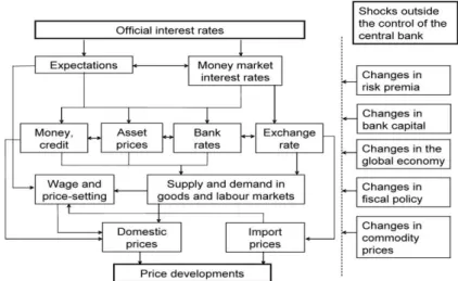
The transmission of the monetary policy to the macroeconomic aggregates is made through several channels as explained in The Monetary Policy of the ECB, published by the European Central Bank (ECB) in 2004 (see figure 3).
Figure 3: Transmission of the Monetary Policy. Source: The Monetary Policy of the ECB, 2004
Changes in the official interest rates of the Central Banks will influence the economic agents’ expectations regarding the future monetary policy and the money market
7 interest rates. These two variables, combined, will influence the main transmission channels which are the credit channel, representing the credit available in the economy, the assets’ price channel, the interest rates channel representing the bank rates charged to households and firms, and the foreign exchange rate channel that affects the relative prices of the imported and exported goods. With all these variables being influenced, they will function as different transmission channels that affect the conditions in the labour market (wages), the supply and demand in the goods and services market (goods and services prices), and the foreign trade, which consequently influence the whole aggregate demand in the economy and, therefore, the evolution of the price level in that specific currency area. All of these channels can be affected by external shocks in the risk premium concerning the economy, in the banking system capital buffers, in the fiscal policy, in the commodity prices and in the evolution of the global economy, which always add uncertainty to the expected transmission of the monetary policy regarding the mid-term evolution of prices.
Despite the main goal of Central Banks being the control of the price level because of the quasi-consensus due to the Neo-Classical/ Neo-Keynesian synthesis that output and unemployment in the long-run cannot be influenced by monetary shocks (Goodfriend, 2007), in transition from the short to the long-run monetary policy can in fact influence variables such as wages or aggregate demand and supply in the goods and services markets. In consequence, the output and the unemployment rate will be affected, which makes relevant the study of the transmission channels and the mechanisms of the monetary policy in the mid-term.
8 One of the transmission channels that we can observe in figure 3 is the Assets Price transmission channel which is important because it involves several sub-channels 3 representing the wide range of assets that can exist in the economy such as: stocks, bonds, real estate, etc. All of these can react in heterogeneous ways to changes in Central Banks’ official rates. Due to this heterogeneity our study will be focused on the reaction of the equity price sub-channel to changes in the Central Banks’ official interest rates.
In a conventional monetary policy situation, i.e., a situation in which the asset price transmission channels and, more specifically, the stock price sub-channel react to changes in the official interest rates of the Central Bank, it is supposed that a higher rate will cause a decrease in the stock price. This relationship comes from the standard financial theory:
(1)
being Po the price of the stock, Rf the risk-free rate and E[Div] the dividends that depend on the expectations regarding the future states of the output in the economy. Analyzing this formula we should assume that the stock price should be neutral in terms of the stock of money in economy. However, several empirical studies state that monetary policy have an impact on stock prices (Cassola and Morana, 2002; and Rigobon and Sack, 2002) either because monetary policy has real effects on future cash flows or because lower interest rates lower the risk-free rate (Thorbecke, 1997).
The stock prices will therefore operate as a monetary policy channel in four different ways: stock prices will affect investment, firms’ balance sheets, household wealth and household liquidity (Mishkin, 2001).
3 Transmission sub-channel of monetary policy is a channel that is part of one of the four main
transmission channels (credit, bank interest rates, assets price and exchange rate) but that has an autonomous way to influence monetary policy within that umbrella channel.
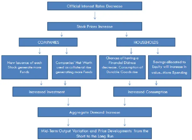
9 Stock prices influence firms’ investment because if an expansionary monetary policy is implemented by the monetary authority raising equity prices, then issuing a stock in order to finance their investment becomes cheaper. This is so because the value of the company is now perceived as higher by the investors and, consequently, they are willing to pay more for each issued share which will increase the company’s funds available for investment. Stock prices also influence firms’ balance sheets because when stock prices rise then the Net Worth of the company used as collateral to banks’ loans will also increase, allowing companies to borrow more funds to invest. Stock prices affect consumer’s liquidity because if equity prices rise, then having a financial distress in the near future will become less probable, so they will be willing to increase the consumption of durable goods and real estate. Finally, stock prices can operate as a monetary channel through their influence on household wealth. If stock prices rise, families’ that have their savings allocated to stocks will increase their wealth and therefore their consumption will rise as well. In these four ways stock prices influence either firms’ investment or household’s consumption. The underlying idea is that an increase in investment and consumption will stimulate aggregate demand and consequently increase output. Figure 4 summarizes the processes described
10 above.
Figure 4: Monetary Policy Stock Price Transmission Sub-Channel. Source: The Author
This is the conventional way how monetary policy is transmitted across the stock prices channel throughout the economy and its several sectors and agents.
However, Central Banks face a serious problem regarding their operational activity when they are confronted with a situation in which their official and main monetary policy tool, the official interest rates are no longer available.
This scenario may happen when economies face the Zero Lower Bound (ZLB), or as it is also known in the economic literature the Liquidity Trap. This is a situation in which the traditional monetary policy tools that are the Central Banks’ nominal official interest rates are no longer effective because the real interest rate that equals the agents’
11 expectations regarding inflation is still too high to assure full employment and price stability. As the nominal interest rates (i) cannot be dropped any further because currency is a store of value and economic agents would not want to deposit an amount A in the present moment to receive A-(A × i%) in the future, Central Banks just cannot keep on using such monetary tool, although there have been Central Banks’ experiences in that field like the Danish Central Bank’s deposit facility that was set into -0.2% in July 2012. In the economic theory it can be explained because there are costs associated with storing cash by the agents such as mobility, security and uncertainty costs that tend to elevate the will of the agents to deposit cash in financial institutions (Thornton, 1999). Notwithstanding, these are not monetary policies commonly implemented by the Central Banks, even in Zero Lower Bound scenarios.
In such an extreme situation for Central Banks’ operational activity (the ZLB), there is some unconventional monetary policy options referred in the economic literature that can avoid the ineffectiveness of the monetary policy. When Central Banks face a ZLB, alternatives to monetary policy can be: the change in agents’ expectations regarding future monetary policy; allowing an increase in the size of the central bank’s balance sheet (Quantitative Easing) beyond the size that was needed to sustain a zero interest rate policy; or altering the central bank’s assets and liabilities in order to influence the securities and correspondent maturities that households, firms and financial system hold (Bernanke et al., 2004). Those are essentially the unconventional monetary policies alternatives that Krugman (2000) presented as well as Eggertsson and Woodford (2004), although these two authors give special emphasis to the economic agents’ expectations regarding the future monetary policy.
12 Facing a ZLB it is important to understand how the stock price sub-channel reacts to the utilization of unconventional monetary policy tools and how this sub-channel keeps on influencing the economy, because only if the transmission channels and sub-channels keep on operating the way they are supposed to in economic theory, is that the unconventional tools may be used successfully.
Central Banks implement their unconventional tools using their Open Market Operations 4 to rebalance securities and their maturities or to increase Central Banks balance sheets. Usually Central Banks do not purchase all kind of assets because they might be exposed to risky assets (e.g. equity) and if the issuers of those securities defaulted the Central Bank assets would be lower than the liabilities (essentially currency outstanding) unbalancing the relationship between money stock and assets held which would raise the risk of inflation. Therefore, Central Banks purchase almost exclusively government bonds and debt of government-sponsored or public companies, even though in the recent financial crisis the FED purchased Mortgage Backed Securities (MBS) in order to enhance the credit market conditions. The purchases of such securities continuously and in a large scale, will also affect the prices of other assets including stocks.
Large Scale Asset Purchases (LSAP) are the asset purchases that Central Banks carry out through their open market interventions and are used to implement the quantitative easing and the shifting of Central Bank’s balance sheet composition policies. In economic literature we can find several ways throughout LSAP influence the whole asset price channel.
4
Open Market Operations are monetary policy operations carried out by a Central Bank within its operational framework in which the direct intervention of the Central Bank in the Money Market or in the securities’ secondary market play an important role in the orientation of interest rates, the management of the liquidity in the financial system and to signal the future monetary policy.
13 D’Amico et al. (2011), Hancock and Passmore (2012), and Joyce et al. (2011) refer the Central Banks’ signaling that is sent to the market when there is a LSAP’s announcement, as one of the channels throughout the LSAP influence the asset prices. This is so because investors create their expectations about the future monetary stance, macroeconomic policy and the state of the Economy when a Central Bank, with large capacity to intervene in the market, purchase and maintains the yields of a particular security, independently of the market conditions. The announcements also decrease the investors’ apprehension about the effectiveness of a guarantee that authorities give to a specific asset because there is, in fact, an official policy regarding the purchase of that security.
Gagnon et al. (2011) and Joyce et al. (2011) also state that LSAP may influence asset prices by the market functioning/liquidity channel, i.e., as market participants know that the Central Bank is purchasing a large amount of a particular security independently of the market atmosphere, they will be more willing to trade, increasing liquidity in the market which reduces the liquidity risk and therefore reducing the liquidity premium and the overall yields of the asset, which will raise its price.
D’Amico et al. (2011) refer the scarcity effect, in which a Central Bank’s large purchase of an asset will decrease its own specific yield and raise its price due to the preferred habitat theory. This study also refers the duration effect, in which a Central Banks’ large purchase of assets with longer maturities will reduce the overall market maturity which consequently decreases the term premium.
At last, all of the authors cited above refer the portfolio rebalancing effect as one important mechanism to transmit the large scale asset purchases to the asset prices. The main idea is that, as a consequence of all the effects mentioned earlier, and since assets
14 are not perfect substitutes, lower expected returns on the purchased asset (e.g. Treasury Bond) increases the willingness of investors to acquire securities with expected higher returns (e.g. equity).
In the figure 5 we can observe how the LSAP programs may have an impact on the stock market, and after it will be given a concise explanation of all the process represented in the scheme.
Figure 5: Large Scale Asset Purchases (LSAP) Impact on Stock Prices. Source: The author.
The signaling effect represents the confidence that investors have in official policy news regarding the commitment of the Central Bank to a certain type of unconventional monetary policy. The announcement of a LSAP program will influence the investors’ expectations because financial markets are composed essentially by forward looking
15 agents. That announcement should immediately start producing effects on the financial transmission process. This is so, because investors assume that it will exist a strong impact of such a large purchase program on several financial dimensions, such as: the term premium, the liquidity premium and on the supply of the particular type of asset that is going to be purchased. This communication will start to be perceived by the agents as a signal that the yields of the purchased asset will start to fall and their prices will start to rise, and the agents will expect that a monetary expansionary policy will produce a positive impact on mid-term output and cash-flows because of the non-absolute neutrality of money in the transition from the short to the long run. The expectation that the price will start to rise will lead short-term investors to purchase that particular asset because it is known that the Central Bank will be active in that security market regardless of its conditions. This will augment the effect expected by the Central Bank that is the reduction of the overall yields of the large scale purchased asset. The expectation that yields will lower in the mid-term, and the expectation that cash-flows will increase due to the expansionary monetary policy carried out by the Central Bank, will lead mid and long-term investors to start rebalancing their portfolios, purchasing securities with higher expected returns like stocks.
This signaling effect is only effective if the Central Bank program’s credibility is reinforced by a large and real intervention in the secondary market of the securities that were announced to be purchased.
This Central Banks’ intervention in the secondary market for Longer Term Government Bonds will lower the term premium since this purchase program withdraws from the market government bonds with a longer duration that can be perceived by investors as having more duration risk. Also the liquidity premium will decrease because the Central
16 Bank’s intervention will enhance the functioning conditions of the market, allowing investors to trade away their securities, in this case not only Longer Term Government Bonds but also MBS, in every moment and every quantity they feel convenient, reducing trading apprehension and therefore increasing liquidity in the purchased assets markets. Finally, the large purchase of a particular asset by a Central Bank in segmented financial markets, will cause the scarcity of the asset in a specific segment of the market and, therefore, investors that are demanding for assets with that kind of specific features will pay more for the security they prefer, which will rise its price and lower its overall yield.
All these three factors combined will cause a decrease in overall yields of the financial assets purchased by the Central Bank, leading investors to rebalance their portfolio, looking for securities with expected higher returns. Risky assets like stocks historically have a higher return than government bonds, being the post-World War II mean value-weighted NYSE 8% per year over the T-bill rate (Cochrane, 2005). This will induce investors to purchase equity and consequently increasing stock prices.
3. The Impact of the QE Programs on US Equity Market: An
Empirical Assessment
In this chapter, it will be assessed the statistical significance of the FED’s QE programs that were put into practice between January 2009 and March 2010, usually known as Quantitative Easing I (QEI), and from November 2010 to July 2011, usually known as Quantitative Easing II (QEII) on S&P500.
In the QEI Program, the Federal Reserve purchased a large scale of Mortgage Backed Securities, Agency Debt from Freddie Mac and Fannie Mae and Long-Term Treasury
17 Securities to an extent of $1,75 trillion. In the QEII Program the FED only purchased Long-Term Treasury Securities to an extent of $600 billion. These two Programs had two main objectives: enhancing the credit market conditions, through MBS purchases, and to reduce the long-term interest rates in order to stimulate the recovery of North-American Economy, through North-North-American Government Bonds purchases.
Thus, it will be assessed if there is an indirect link between QE programs and S&P500 returns like the one that is presented in the second chapter of this dissertation.
3.1. Empirical Assessment Rationale
The empirical analysis of this research will be based on the Arbitrage Pricing Theory (APT) rationale, that was first developed by Ross (1976) and that is summarized by Huberman (2005).
The APT model consists of a one-period model in which economic agents assume that the stochastic properties of returns of a financial asset are compatible with a factor structure. In this rationale if there is no arbitrage opportunities the financial asset returns will be linear in the factor structure that is represented in the following equation:
(2) ri = µ + 𝛽f + ε,
where ri is the return of the asset i, µ is a constant for that given asset, 𝛽’s are the
sensitivities of the return of the asset i to the factors f that are assumed to influence the return of i and ε is an idiosyncratic random shock with mean assumed to be zero E[ε] = 0.
Assuming i as a risky asset we can take the expectations regarding its returns. Therefore, we can express economic agents’ expectations in the following expression:
18 (3) E[ri] = rf + 𝛽1RP1+ 𝛽2RP2+…+𝛽nRPn,
being E[ri] the expected return of the asset i, rf the risk-free rate, 𝛽’s the sensitivities of
the asset i to a given factor and RP’s are the risk premiums associated with each explanatory factor.
If the agents believe that the pricing of the assets strictly follow an APT rationale they would price all the market securities under the factor structure approach exposed above. Consequently, if an asset diverges from the theoretical price that is calculated using the expected return of a security in the APT model, which implies that either the asset is too expensive or the asset is too cheap, the investor will short-sell the asset, if it is too expensive, and purchase the portfolio of assets that are correctly priced at that moment. At the end of the period the investor should sell the portfolio and purchase back the asset that was mispriced previously earning the difference. This idea can be applied in reverse if the mispriced asset is too cheap in the beginning of the period.
This arbitrage strategy guarantees that the investor will profit a risk-free amount of money without being exposed to the factors’ risk complied in the factor structure of the model. As all the agents behave like the representative agent sooner the expensive financial asset being sold in the market will tend to reduce its price to the price agents believe is fair when they evaluate its value under the APT model, eliminating any arbitrage opportunities and pricing correctly all of the securities in the market.
3.2. Explanatory Variables
As it is exposed by Huberman (2005) there are several approaches to select factors for the linear structure of an APT model. One of the choosing methods consists of picking
19 up factors based on economic intuition and to estimate the factor loadings evaluating if they explain the cross-sectional variations in the expected returns, which was chosen by Chen, Roll and Ross (1986).
As we intend to evaluate the impact of monetary policy instruments on the evolution of the returns of the S&P500, we will start from the macroeconomic and financial variables that these authors found statistically significant to explain the equity returns in the United States of America, and then we measure them together with the Federal Funds Target (conventional monetary policy instrument) and a dummy for the Quantitative Easing Programs periods, in order to obtain an econometric model that consists only of macroeconomic, monetary and financial explanatory variables.
The main idea is that the macroeconomic, financial and monetary variables chosen can explain the returns in North-American equity markets, based on the following identity,
(4) ,
where E(c) are the expected cash-flows, k is the discount factor and P the stock price. In the APT spirit, Chen, Roll and Ross (1986) conclude that the North-American equity market returns could be expressed using the following linear equation
(5) R = α + βMpMP + βDEIDEI + βuiUI + βUPRUPR + βUTSUTS + ε
where R represents the stock market returns and βMp, βDEI, βui, βUPR and βUTS represent
the sensitivity of the stock market returns to the industrial production, to the changes in expected inflation, to the unexpected inflation, to unexpected changes in risk premium and to shape of the term structure, respectively.
The set of regressions that will be tested in chapter 3.5 will have the following rationale (6) R = α + βmvMV + βfvFV + βfftFFT + βqeQE + ε
20 where βmv, βfv, βfft andβqe represents the sensitivity of the stock market returns (R) to
the macroeconomic and financial variables present in equation 5 (MP, DEI, UI, UPR and UTS), and to the Federal Funds Target (FFT) and the QE programs (QE), respectively.
3.3. Series
The series were created based on the methodology developed by Chen, Roll and Ross (1986) with several differences because new series are now available regarding inflation and the component of the risk premium variable.
The financial data for the R variable which represents the returns of the North-American equity market, was obtained from the web site Yahoo Finance and the series chosen was the S&P 500 index.
The data to compute the Monthly Growth of the Industrial Production (MP) was collected from the Federal Reserve of St. Louis Database (FRED). The series selected was the Industrial Production Index of the Board of Governors Federal Reserve System on a monthly basis because this is the highest frequency available on the data. The Monthly Growth of the Industrial Production (MP) will be given by the following formula
(7) MPt = log (IPt/IPt-1),
and as the Industrial Production Index represents the flow of production of a specific month, its influence will only be effective in the following month after the release of the periodic report . Consequently we have to consider the existence of one month lag in this variable.
21 The series of the Changes in Expected Inflation (DEI) was computed using the data available in the Cleveland FED Database. Cleveland FED computes a monthly series with the expected inflation for different time horizons from January 1982 to the present moment.
Our formula will be as following: (8) DEIt = E [It+12|t] – E [It+12|t-1].
DEIt will represent the monthly change in the expected inflation for the next year, which
is more forward looking than the change of expected inflation for each month ahead considered by Chen, Roll and Ross (1986). In our point of view a variable considering changes in expected inflation for each following month would have less economic meaning than our variable, because it seems more difficult to assume that the economic agents create expectations for each month ahead and not for the whole year.
The variable Unexpected Inflation (UI) is also computed using the data available in the Cleveland FED Database for the expected inflation. The effective annual inflation data was calculated from the Current Consumer Price Index published monthly by the Bureau of Labour Statistics (BLS) of the United States of America. As a consequence, our variable will be constructed using the following expression:
(9) UIt= It – E [It|t-12].
Therefore, UIt will represent the difference between the annual inflation that was
effectively observed for the month t comparing with the expectation that existed in the market for the one year ahead inflation in the analogous month of the previous year. The explanatory variable that represents the unanticipated changes in risk premium (UPR) was computed following the same equation:
22 We collected the monthly data for the Moody’s BAA Corporate Bond Yield and for the 10-Year Treasury Constant Maturity Rate (proxy for the LGB) from the Federal Reserve of St. Louis Database (FRED).
The Term Structure (UTS) and it is computed as follows: (11) UTSt = LGBt – TBt-1,
where LGBt represents the same series as the one used in the Risk Premium calculation
and TB represents the Treasury Bill Rate in the previous month which allows us to capture shifts in the yield curve structure. The proxy for the Treasury Bill Rate is the 3-Month Treasury Bill Rate in the Secondary Market collected from the Federal Reserve of St. Louis Database (FRED).
In order to evaluate the impact of the QE programs and the whole impact of the Monetary Policy in the North American Equity Markets we need to create proxies for this monetary policy instruments and to include it in the APT based model that we mentioned previously.
The variable representing the conventional monetary policy will be the monthly FED Funds Rates Target (FFT). Once again we extract this monthly series from the Federal Reserve of St. Louis Database (FRED).
At last, the proxy that will represent the unconventional monetary policy actions carried out by the FED since the beginning of the Sub-Prime Crisis will be a dummy (QE) that has the value 1 in the months when the QE programs were active and the value 0 when the programs where inactive. The Data on those months was picked from the New York Federal Reserve website.
23
3.4. Methodology
In order to assess the statistical significance of the loading factors represented by the explanatory variables in the previous sections, we will use a Generalized Autoregressive Conditional Heteroskedasticity (GARCH) model since these econometric models allow us to have a linear equation for the mean but a non-linear equation for variance that will be interpreted as the weighted function of a long-term average value of the variance. It will be used a GARCH (1, 1) model meaning that the current conditional variance can depend on 1 lag of the squared error and 1 lag of conditional variance. Since there are only 3 parameters included in the conditional variance (Equation 12 presented below) this kind of models are very parsimonious because “allow an infinite number of past squared errors to influence the current conditional variance” and “in general a GARCH (1,1) model will be sufficient to capture the volatility clustering in the data and rarely is any higher order model estimated” (Brooks, 2008).
We do not assume a constant value for the variance but simply we assume that the conditional variance is given by the following equation,
(12) t= α0 + α1 t−1+ β t−1
implying that the present variance depends on the square of the residuals of the previous period and on the previous value of the conditional variance. The conditional variance changes over time but the unconditional variance of the residuals given by
(13) VAR(ut)=α0/(1-(α1+β))
under a GARCH (1, 1) specification, is constant as long as α1+β 1.
Financial series usually present a variance pattern that changes with time, having volatility clusters and therefore, the assumption present in the Classic Linear Regression
24 Model, that should exist homoscedasticity in order to obtain a Best Linear Unbiased Estimator, i.e., the error term must exhibit a constant variance, would not be satisfied. In our specific case we will include exogenous variables in the variance equation and in the mean equation. The monetary policy tools (conventional or unconventional) will be tested in order to know if they have, not only an impact on the returns of the US Equity Market (observable when we define the mean equation), in our study represented by the S&P 500 index, but also on the volatility of this index (observable when we define the volatility equation). Therefore, the GARCH model will allow us to make inference about the volatility pattern and the factors that explain the evolution of the returns of the S&P 500 index.
We will have a more accurate estimation because we account for the heteroskedasticity in the financial series and at the same time the GARCH model gives us more information about the interaction of the variables studied, i.e., how monetary policy affects the volatility in the equity markets.
As we can see by the following figure, the returns of the S&P 500 on a monthly basis from January 1988 to September 2012, followed a volatility clustering which is “[…] the tendency of large changes in asset prices (of either sign) to follow large changes and small changes (of either sign) to follow small changes. In other words, the current level of volatility tends to be positively correlated with its level during the immediately preceding periods” (Brooks, 2008).
25 -.10 -.08 -.06 -.04 -.02 .00 .02 .04 .06 88 90 92 94 96 98 00 02 04 06 08 10 12 RSP500
Figure 6: Monthly S&P 500 returns for January 1988 to September 2012. Source: Yahoo Finance and Author Calculations
We will use monthly data in order to allow us to include essential macroeconomic variables that have no higher frequency (e.g. Industrial Production and Inflation Rates) This date range will be divided in sub-periods in order to allow the model to capture structural changes in the relation between the returns of the S&P500 and macroeconomic and monetary variables across the period of analysis.
The date range considered in the present research will be from January 1988 to September 2012. This period was chosen because it gives us a sufficiently large period of time for monthly data and represents the period after the two oil-shocks of 1973 and 1979 which were characterized by the expressive rise in the inflation rate in the United States of America during the 70’s and early 80’s. This fact turned the main concern of the FED in the control of the excessive rise in the price level during the time Mr Paul Volcker was in office (1979-1987). Thus, our period of analysis will focus on the new paradigm of monetary policy which was characterized by low inflation and interest rates
26 during the 90’s and the first decade of the XXI century, period in which Mr Alan Greenspan was the Chairman of the Federal Reserve.
In the next section of this chapter, we will present the specification and results of our regressions based on the GARCH Model that was previously explained.
3.5. Empirical Results
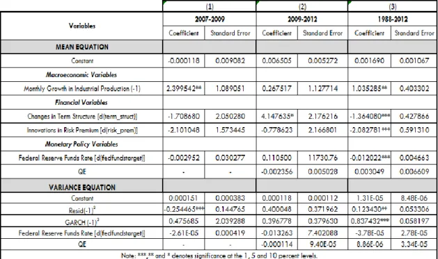
In the first set of regressions (table II) we evaluate if the macroeconomic, financial and conventional monetary policy variables presented previously are significant to explain the evolution of the S&P500 index. In the second group of regressions (table III, IV and V) it will be assessed if the unconventional monetary policy instruments (QE) had a direct impact on the S&P500 returns and if they were able to keep the stock price transmission sub-channel effective.
Table II: GARCH Regression of the returns of the S&P500 Index, January 1988- September 2012. Source: Author’s Calculation
27 In the first regression present in Table II, it was tested if the macroeconomic and financial variables were significant in our period of analysis.
As we can observe the variable Changes in Expected Inflation was not significant. This is due to the fact that it has shown little volatility during the period of our analysis. This evidence is in line with Chen, Roll and Ross (1986) in which they found that the inflation related variables were only significant in periods when these variables were highly volatile. This is not the case in our period (1988-2012) in which the expected inflation volatility was only 0.31%. Even if Unexpected Inflation does not show such a low volatility as Changes in Expected Inflation, it was still little volatile in the period (1.24%). This fact, allows us to exclude Unexpected Inflation from our next regressions, because when we include monetary policy variables (second regression in Table II) it also loses its explanatory power within the model. Thus, both inflation-related variables become non-significant econometrically, as it can be observed in the second mean regression in the table. This exclusion will allow us to have a more accurate and parsimonious model.
The third regression Table II includes only the financial, monetary and macroeconomic significant variables which are: the innovations in the risk premium, the innovations in the term structure, the monthly growth of industrial production with a one-period lag and the innovations in the Federal Funds rate target which is our proxy for the conventional monetary policy.
In this same regression it is also observable that a positive change in the term structure causes a decrease in equity market returns. This relation occurs because if the long-term rate of the US Treasury securities falls, all the interest rates tend to fall for any form of capital. Consequently, investors will allocate their savings in assets that offer protection
28 against this event. These assets are the ones whose price increases when long-term real rates decline (Chen, Roll and Ross, 1986). Empirically stocks follow this pattern.
Also, as it is evident in the same regression, when we consider the whole period, the innovations in the Federal Reserve funds rate target were significant and they have a negative impact on the returns of the S&P500 index. This negative impact is in line with the standard financial theory that states that an increase in the FED’s funds target rate will increase the costs of banks to finance themselves in the Central Bank, which will affect the amount of money they are willing to lend the economy. Consequently, consumption, investment, cash-flows and dividends will fall. The monthly growth of the production index has a positive sign. This is so because an increase in the industrial production is a proxy for the increase of the total output in the economy. Aggregate production generates cash-flows and dividends that drive stock prices up.
We can also observe that the innovations in the risk premium have a negative impact on the returns of the S&P 500. An increase in the risk premium causes a decrease in the equity market returns because such a rise represents that the preferences of the investors for risk-free assets is increasing. This fact decreases the amount of cash invested in riskier assets such as stocks.
At last we can observe that all the explanatory variables are significant at a 1% significance level in the mean equations and that in all the variance equations of the regression, the Federal Funds rate target did not have any impact on the volatility of the S&P500 index during the period between 1988 and 2012.
In Table III, it is assessed if during the period of time between 2007 and 2009 and between 2009 and 2012, the FED was able to keep the equity price transmission sub-channel active. In the first period, the decrease of the Federal Funds target rate was the
29 only mechanism used and in the second period the FED implemented the Quantitative Easing programs. It is also assessed if the QE programs have any direct impact on the S&P returns when it is considered a longer period of time (1988-2012).
Table III: GARCH Regression of the returns of the S&P500 Index, January 1988- September 2012, July 2007- September 2012 and January 2009- September 2012. Source: Author’s Calculation
In the first regression present in Table III we considered only the period ranging from the beginning of the subprime crisis in July 2007 until the beginning of the first Quantitative Easing program in January 2009. During this period of time, the FED lowered the Federal Funds Rate target from 5.25% to the range 0-0.25%. Therefore, we assess if there is statistical evidence that the conventional monetary policy lost its capacity to influence the evolution of the stock market returns. The results in regression 1 suggest that the stock price transmission channel of the conventional monetary policy became ineffective in the period after the Subprime crisis, since it appears that the link
30 between the Federal Reserve funds target and the equity price transmission channel was lost after 2007.
Despite the efforts of the FED to turn the monetary policy effective again, with the implementation of the QE programs in January 2009, these unconventional monetary instruments did not appear to have any direct impact on the stock price transmission sub-channel since in the second mean equation present in Table III, the QE coefficient is non-significant statistically.
The third regression allows us to conclude that in a longer term perspective (1988-2012) only the conventional monetary instruments were able to influence the North-American Equity Market directly.
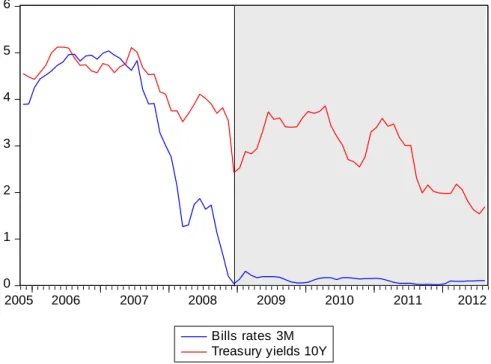
When we consider the period after the launching of the QE programs (from 2009 onwards) it is easily observed in the second regression present in Table III that the only significant variable influencing the evolution of the equity prices were the innovations in the term structure. An increase on the Term Structure of 1 p.p. increases the monthly returns of the S&P500 Index in 4.14 percentage points. It can be noticed that the signal of the term structure variable changed from negative to positive. This happens because the short-term Treasury Bill yield (3 months maturity) lowered in a larger and more permanent scale than the longer term one (10 year Treasury Bond). This yield pattern, shown in Figure 7, seems to appear because in a period of such a financial distress, even if the longer term government securities yields fall because of the FED’s large scale purchase, the short-term yields experience a more intense decrease because they became perceived as the best risk-free asset.
31 0 1 2 3 4 5 6 2005 2006 2007 2008 2009 2010 2011 2012 Bills rates 3M
Treasury yields 10Y
Figure 7: Evolution of the 3Month US Treasury Bills and 10 Years US Treasury Bonds
The QE programs had the direct objective of enhancing the credit market conditions through the large purchase of MBS and in an even larger scale, Longer-Term Government Securities. Therefore, if these programs were successful Changes in Term Structure variable should be influenced by the purchase of the Longer-Term Asset Purchase implemented by the FED.
In Table IV it can be observed that the Quantitative Easing programs had in fact a significant impact on the increase of the term structure at a 1% significance level, during the period they were active.
32
Table IV: GARCH Regression of the returns of the Changes in Term Structure, and January 2009- September 2012. Source: Author’s Calculation
Analysing the QE coefficient in the Table IV we can observe that per each month the QE program was active there was an increase of the Term Structure in 0.0027 percentage point. We can also observe that the Federal Funds Rate target was non-significant statistically indicating that the Federal Reserve Quantitative Easing Programs were effective on their main objective of impacting on the term structure, but with a different signal than the one we could initially expect.
Observing the previous results in Table IV (QE programs impacted on the term structure) and comparing them with the results shown in Table III (the term structure impacted on the equity market) one could suppose that may exist a link between the months while the Quantitative Easing programs were active and the increase on the S&P 500 index returns through the impact of these programs on the Changes in Term Structure.
In Table V it is tested the direct impact of the months when the QE programs were active on the returns of the S&P500 without any other variables included in the
33 regression. This is done in order not to have a statistical indirect impact of other variables through the inclusion of redundant regressors or variables that are correlated with the QE dummy such as the Changes in Term Structure.
Table V: GARCH Regression of the returns of the S&P 500 Index, January 2009- September 2012 and January 1988-September 2012. Source: Author’s Calculation
It is observed that the QE programs showed no evidence of influencing the S&P 500 returns during the period while they were active (2009-2012) and in a longer term perspective (1988-2012). Therefore, from the results in the tables shown above one can conclude that, in our model, we find no evidence that the Federal Reserve’s Quantitative Easing Programs had an impact on the monthly returns of the S&P500 Index, our proxy for the North American equity market.
34
4. Conclusions
It can be concluded from our research that in a long term perspective, from 1988 to 2012, the monthly growth of industrial production, the innovations in the risk premium and the changes in the term structure, impacted on the monthly returns of the S&P 500 index, our proxy for the North-American Equity market. The inflation related variables remained less effective because there was less volatility in these regressors during our period of analysis, which is in line with Chen, Roll and Ross (1986).
It can also be concluded that in that same time horizon (1988-2012) the changes in the Federal Funds rate target (the proxy for the conventional monetary policy) were effective in influencing negatively the monthly returns of the S&P500, as it is expected in the economic theory (Cassola and Morana, 2002; Rigobon and Sack, 2002; and Thorbecke, 1997).
However, after the beginning of the subprime crisis, in July 2007, one can conclude that the innovations in the Federal Funds rate target ceased to have impact on the S&P500 index as the North American Economy started to face the Zero Lower Bound (ZLB). The conventional monetary policy instruments lost their power to influence the several transmission channels, and the asset price sub-channel was also affected. This ineffectiveness of the monetary policy is well documented in the economic literature and is also known as the Liquidity Trap.
This situation can be reversed if unconventional monetary policy instruments are put into practice by the Central Banks, such as Quantitative Easing Programs that cause changes in the agents’ expectations and in the Central Banks’ Balance Sheets (Krugman, 2000 and Eggertsson and Woodford, 2004).
35 In the regressions presented earlier it was found evidence that these unconventional programs impacted on the Changes in The Term Structure during that period proving that QE was important to enhance the credit market conditions. This fact is in line with the main objective pointed by Mr Bernanke when the FED launched these programs in 2009. This conclusion is also present in others authors’ researches (Gagnon et al., 2010, Hancock and Passmore, 2012, and Breedon et al., 2012), although, in our results, it seems that the QE programs had more impact through the stabilization of the short-term yields in reduced levels, than through the lowering of longer-term yields.
It is also observable that the Change in the Term Structure was the only explanatory variable that remained significant during the two QE programs. The fact that the term structure has shown a positive sign during this period suggests that, although both long and short term bonds’ yields have fallen after the QE programs were launched, the investors started to purchase more stocks when the difference between the long term Treasury Bond yields and the risk free asset yield (3 month Treasury Bill) increased. This seems to have happened essentially due to the decrease of the 3 month Treasury Bill rates to values near zero in a more permanent and more stable manner than the 10 Year Treasury Bond yield.
However, in the regressions presented above it was found no evidence that the Quantitative Easing Programs had a direct influence on the monthly returns of the S&P500 index from 2009 to 2012. This is in line with what Breedon et al. (2012) found in their research for the British stock market during the Bank of England QE program. As in the present research, the authors found that the QE programs had impacted on the government bonds’ prices and yield (in the present research represented by the Changes in Term Structure) but showed a limited impact on other financial assets like stocks.
36 Joyce et al. (2011) also concluded that the impact of Bank of England’s QE programs on the British equity market after March 2009 was highly uncertain, since in their research, different approaches retrieved substantial different results and magnitudes of the impacts.
In short, it can be concluded that during the first and second FED’s QE programs the variable that most influenced the monthly returns of the S&P500 Index was the Changes in the Term Structure due to the decrease and stabilization of the 3 month Bill rate near zero. As the QE programs were focused essentially on the large scale purchase of longer term Treasury bonds it was found no direct relation between the implementation of these programs and the increase of the North-American stock prices after March, 2009. As the Changes in Term Structure happened essentially due to the stabilization of the risk free rate near zero, one can conclude that the financial standard theory gives us the answer for a part of the performance of the North-American equity market after 2009, because when investors discount the future cash-flows at a lower rate, the present value of future dividends increases, increasing the present value of the stocks.
Nevertheless, in future research, it is important to understand the direct impact of the Quantitative Easing programs on the short term bills rates and, through this channel, assess the indirect impact of the QE programs on the performance of the North-American equity market after 2009. Also, in the APT rationale that was the framework to our empirical research, it would be important to develop further investigation on the causes that could explain the performance of the North American stock market in the period between 2009 and 2012 (QEI and QEII programs). In order to do so, it will be relevant to include in a GARCH model other economic and financial variables that were not tested in the present research, or other proxies for the unconventional monetary
37 policy, such as higher frequency data like the daily purchase of North-American or the daily or weekly change in Federal Reserve balance sheet composition.
38
5. References
Bernanke, Ben S. (2009). The Crisis and the Policy Response, Speech presented at the Stamp Lecture, London School of Economics, London, England.
Bernanke, Ben S., Vincent R. Reinhart, and Brian P. Sack (2004). Monetary Policy Alternatives at the Zero bound: An Empirical Assessment, Brookings Papers on Economic Activity, Issue 2, 1-100.
Breedon, F., Chadha, J.S. and Waters, A. (2012). The Financial Market Impact of UK Quantitative Easing, BIS Papers chapters, in: Bank for International Settlements (ed.), Threat of fiscal dominance ?, volume 65, pages 277-304 Bank for International Settlements.
Brooks, Chris (2008). Introductory Econometrics for Finance, second edition, Cambridge University Press, Cambridge
Cassola, N. and Claudio M. (2002). Monetary Policy and The Stock Market in The Euro Area. Working Paper No.119, European Central Bank.
Chen, N., R. Roll, and S. A. Ross (1986). Economic Forces and the Stock Market, Journal of Business, 59, 383–404.
39 Chicago Board Options Exchange (2013). CBOE Volatility Index (VIX) [On Line], Retrieved from: http://finance.yahoo.com/q?s=^VIX, [Accessed at: 2013-02-20]
Cochrane, J. H. (2005). Asset Pricing, Revised Edition, Princeton University Press, Princeton.
D’Amico, S., English, W., Lopez-Salido, D. and Nelson, E. (2011). The Federal Reserve’s large-scale asset purchase programs: Rationale and effects, Working Paper, Board of Governors of the Federal Reserve System.
Eggertsson, G.B. and Woodford, M. (2004). Policy Options in a Liquidity Trap, American Economic Review, 94(2), 76-79.
European Central Bank (2004). The Monetary Policy of the ECB, Frankfurt: European Central Bank
Federal Reserve Bank of Cleveland 2013). Cleveland Fed Estimates of Inflation
Expectations [On Line], Retrieved from:
http://www.clevelandfed.org/research/data/inflation_expectations/index.cfm [Accessed at 2013-05-09]
Federal Reserve of New York (2013). Federal Funds Data [On Line], Retrieved from: http://www.newyorkfed.org/markets/omo/dmm/fedfundsdata.cfm [Accessed at: 2013-05-09]
40 Federal Reserve of St. Louis (2013). Federal Reserve Economic Data- FRED [On Line], Retrieved from: http://research.stlouisfed.org/fred2/ [Accessed at: 2013-05-09]
Gagnon et al. (2011). Large-Scale Asset Purchases by the Federal Reserve: Did They Work?, Staff Report no. 441, Federal Reserve Bank of New York, Staff Reports
Goodfriend, Marvin (2007). How the World Achieved Consensus on Monetary Policy, Journal of Economic Perspectives, 21(4): 47-68
Hancock, Diana, and Wayne Passmore (2012). The Federal Reserve’s Portfolio and its Effects on Mortgage Markets, Finance and Economics Discussion Series 2012-22. Washington: Board of Governors of the Federal Reserve System.
Huberman, Gur (2005). Arbitrage pricing theory, Staff Report, Federal Reserve Bank of New York, No. 216
Joyce et al. (2011). The financial market impact of Quantitative Easing, Bank of England Working Paper No. 393
Krugman, P. (2000). Thinking about the Liquidity Trap, Journal of the Japanese and International Economies, 14, 221-237.
41 Mishkin, F. (2001). The Transmission Mechanism and the Role of Asset Prices in Monetary Policy, NBER Working Paper no 861.
Rigobon, Roberto, & Sack, Brian. (2002). The Impact of Monetary Policy on Asset Prices. Finance and Economics Discussion Series 2002-4. Board of Governors of the Federal Reserve System.
Ross, S. (1976). The Arbitrage Theory of Capital Asset Pricing, Journal of Economic Theory 13, 341–60.
Standard & Poor’s (2013) . S&P500, Stock Market Index Quote, Yahoo! Finance, Retrieved from: http://finance.yahoo.com/q?s=^gspc [Accessed at: 2013-05-09]
State Street Corporation (2013). Investor Confidence Index [On Line], Retrieved from : http://statestreetglobalmarkets.com/research/pdf/historicaldata.pdf, [Accessed at: 2013-02-20]
Thorbecke, Willem (1997). On Stock Market Returns and Monetary Policy. Journal of Finance, 52(June), 635-54.
Thornton, Daniel L. (1999). Nominal Interest Rates: Less than Zero? , Federal Reserve Bank of St. Louis Monetary Trends (January 1999), 1.
42 U.S. Bureau of Labor Statistics (2013). Consumer Price Index History Table [On Line], Retrieved from: ftp://ftp.bls.gov/pub/special.requests/cpi/cpiai.txt [Accessed at: 2013-05-09]