1
A Work Project, presented as part of the requirements for the
Award of a Master Degree in Economics from the NOVA –
School of Business and Economics and Insper Institute of
Education and Research.
DO INDUSTRIES LEAD STOCK MARKETS IN BRAZIL?
RAPHAEL BENO CITRON (26349)
A Project carried out on the Master in Economics Program,
under the supervision of: Martijn Boons and Ricardo D. O.
Brito.
2 Do Industries Lead Stock Markets In Brazil?
Abstract
Hong et al. (2007) claim that a number of industry returns in U.S. and in eight largest non-U.S. stock markets can forecast the stock market using monthly data. Tse (2015) reexamine their results in U.S. with updated data and extended period, he finds evidence that the market can predict industries more significantly than can the reverse. I investigate these relationships for the Brazilian market, adding a study to check if the causality from industries to the market is independent of the chosen model. Data is from August of 1994 to September of 2016. I found that isn’t possible to conclude that industry returns causes stock market returns for Brazil. I also show that the forecasting power that some models may present isn’t robust to a sub-sample analysis. My overall results are consistent with the efficient market hypothesis.
Keywords: Asset Pricing, Information and Market Efficiency, Financial Markets and Macroeconomy, International Financial Markets
JEL: G12, G14, E44
1. Introduction
The efficient market hypothesis is that prices fully and quickly reflect all available information. This study is based on theories that explore the implications of limited information-processing capacity for asset prices. Investors are better characterized as being boundedly rational (Shiller (2000), Sims (2001)). In other words, traders have a limited ability of paying attention to all sources of information much less understand their impact on the prices of the assets that they trade.
I repliacate part of the paper “Do Industries Lead Stock Markets? Hong, Tourous, Valkanov (2004)”, for the Brazilian market (from now on HTV). In the paper the authors test the hypothesis that industry portfolios are able to predict the movement of stock markets and economic indicators. For the U.S. case, HTV find that some industry portfolios forecast the stock market by up to two months. The predictive power is due to the correlation of the industry portfolios with economic activity indicators such as industrial production growth. The purpose of this Thesis is to test the ability of Brazilian industries portfolios of leading the stock market and some economic indicators. This present study will also include a causality investigation as suggested by Tse (2015) in “Do industries lead stock markets? A reexamination” (from now on TSE).
The predictability of industry portfolios can be useful in many ways. Traders and portfolios managers would have the ability to improve their portfolios with a higher Sharpe ratio, i.e. hedge funds that have in their mandate market timing would benefit from knowing which industries have forecasting power and the exact time of the impact. It can also help economist investigating economic activity, since industry portfolios can be used as instrumental variable.
The paper also shed some light on the information diffusion theory quoted above. It can be viewed as an empirical evidence of these theories, to the Brazilian financial market. As HTV explained, there is a large literature in psychology that documents the extent to which even attention is a precious cognitive resource (Kahneman (1973), Nisbet and Ross (1980), Fiske and Taylor (1991)), predictability in
3 industry portfolios can be understood as an evidence of human inability of paying attention at a large set of information.
I found that, for Brazil, isn’t possible to conclude that industries portfolios returns cause stock market returns. Like TSE and different than HTV I analyze the causality in the opposite direction, from the market to industries. The predictability that some models may present isn’t robust to a sub-sample analysis. I also didn’t found any evidence that the predictability of industries portfolios is correlated with economic activity indicators.
In Section 2 I review some literature that based HTV and the work of TSE, who criticized the way that HTV tested causality. In Section 3 I present the model and methodology, first I present the theoretical model that can make predictability in industries portfolios to exists, then I present the empirical models that can be estimated to test the propositions. In Section 4 I explain the data that was used and its sources. In Section 5 I present, the results of the many models, the causality between market returns and industries portfolios and a correlation study between economic indicators and the coefficients of lagged industries returns. In Section 6 I check if the results of the previous section are robust to sub-sample analysis. In Section 7 I conclude and compare the results with HTV and TSE.
2. Literature Review
The theory that HTV use is based on Hong and Stein (1999) and Merton (1987). The first one develop a dynamic model of a single asset in which information gradually diffuses across the investment public and investors are unable to perform the rational expectations trick of extracting information from prices. The consequence is that price under-reacts to the information and there is stock return predictability. The last one develops a static model of multiple stocks in which investors only have information about a limited number of stocks and only trade those they have information. As a result, stocks that are less recognized (small trading volume and research coverage) by investors have a smaller investors base and trade at a greater discount because of limited risk –sharing.
The hypothesis that guided the authors is that the gradual diffusion of information across asset markets leads to cross-asset return predictability. Certain investors, such as those that specialize in trading the broad market index, receive information from particular industries only with a lag. This hypothesis relies on two key assumptions. The first is that valuable information that originates in one asset market reaches investors in other markets only with a lag. The second assumption is that because of limited information-processing capacity, many investors may not pay attention or be able to extract the information from asset prices of markets that they do not specialize in.
HTV find that in US, real estate, mines, apparel, print, petroleum, leather, metal, transportation, utilities, retail, money or financial and services have t-statistics of the corresponding lagged industry return that are greater than 1.96 in absolute value (significant at 5% level). Two additional industries, non-metallic minerals, and television have a t-statistics of about 1.7 (significant at 10% level), there are a total of fourteen that can significantly predict the market. The regressions make economic sense, i.e. the lagged returns of petroleum and metal industry portfolios are negatively related to the next period’s market return, this happens because a commodity price shock led to an economic downturn.
4 The authors find that regressions with longer horizons, with market return lagged in more than one month, only four industries are significant at 10% level and none at 5% level, this is consistence with the information taking about two months to be completely incorporated from industries into the broad market index.
Previous studies like (Fama and French (1989)), (Fama and Schwert (1977)), (Campbell and Shiller (1998)), have demonstrated the predictive power of inflation, the default spread, the market dividend yield and the term spread. These variables are related to time varying risk, HTV suggest that lagged industry portfolios are not a proxy to that and capture different factors.
HTV find that twelve of thirty-four industries have predictive power over Industrial Production, this result is in line with Lamont (2001), who finds that portfolios formed from industry returns can track various economic variables like industrial production growth, inflation and consumption growth. Industries that forecast the market also forecast industrial production growth. Similar results were obtained using Stock and Watson Coincident Index. Eight industries are able to forecast market fundamentals at 10% significance level and five at 5% significance level.
When extending the empirical analysis to the rest of the world, HTV find that across the eight countries the UK and Japan have the smallest proportion of significant industries (8 out of 34). Australia and the Netherlands have the most (18 out of 31 and 16 out of 29, respectively). The numbers for IPG (Industrial Production Growth) are comparable, which lead to a similar conclusion of the US case.
A recent study by Tse (2015) argues that using an extend period, 1946-2013, and data, 48 industries, only between one to seven industries have significant predictive ability for the stock market, depending on the significance level and the model specifications. The author argues in favor of the opposite predictive direction from the stock market to industries. In this way, results are consistent with the efficient market hypothesis.
Different than HTV, TSE uses Granger causality to investigate the relation between the market and industries with the Newey-west correction for heteroscedasticity and autocorrelation.
3. Model and Methodology
Theoretically, HTV proposes a model consisting of the pricing of two assets (stocks) in a three-date economy, t = 0, 1, 2, they assume that the risk free rate is zero. The two assets, X and Y, have terminal values at t=2 given by 𝐷" and 𝐷#, which are
jointly normal with means of zero and variance 𝜎%
&,( and 𝜎%),( and covariance 𝜎&),(.
Investors participate in either market X or market Y, this limited participation is due to taxes and regulations.
At t=1, investors in market X receive signal 𝑆& = 𝐷"+ 𝜀&,/ about the terminal
value of X, investors in market Y receive signal 𝑆) = 𝐷)+ 𝜀),/ about the terminal
value of Y, and these signals are known to all participants at t=2, this is the gradual-information-diffusion assumption. The noise in the signals is normally distributed and the errors are independent of each other and of all other shocks in the economy. The supply of assets is assumed to be 𝑄" and 𝑄# shares outstanding for assets X and Y,
respectively.
HTV assumes that investors have CARA preferences with a risk aversion coefficient of 𝑎. Given the price function 𝑃3,4, the investor in asset market 𝑘 ( 𝑘 = 𝑋, 𝑌 )
5 Max 𝐸3,:[-exp(-a𝑊3,%)], k=X,Y,
{θ3}
s.t 𝑊3,4 = 𝑊3,4=>+ θ?,@=>(𝑃3,4 − 𝑃3,4=>),
where 𝑊3,4 and θ3,4 are the wealth and the share holdings of a representative investor
in asset market k at time t and 𝑃3,%= 𝐷3.
The equilibrium price in market k is given by: 𝑃3,4 = 𝐸3,4 𝐷3 − 𝑏3,4𝑄3, k = X, Y,
where 𝐸3,4 𝐷3 is the conditional expectation of the terminal payoff of asset k at time
t, 𝑏3,4 > 0 is the standard risk discount at time t, and 𝑄3 is the supply of the asset.
Given the equilibrium prices form the model above the serial and cross-serial correlations for assets X and Y are self-explanatory and two propositions arose.
Proposition 1: The own serial return correlations are zero, i.e., Corr( 𝑅3,%, 𝑅3,>) = 0 for
K = X, Y. The cross-serial return correlations, Corr(𝑅),%, 𝑅&,>) and Corr(𝑅&,%, 𝑅),>) are
non-zero and can be positive or negative depending on the sign of the covariance of asset payoffs, 𝜎&),(.
Proposition 2: Even if there are arbitrageurs who trade in both markets to exploit the
cross-predictability, as long as there are limits to arbitrage, some cross-predictability will remain in equilibrium.
Empirically, the authors test two specific testable predictions that are implied by the model. Thinking on the broad market index as asset Y and an industry portfolio that is informative of market fundamentals as asset X.
Prediction 1: The broad market index can be predicted by the returns of industry
portfolios, controlling for lagged market returns and well-known predictors such as inflation, the default spread, and the dividend yield.
Prediction 2: The ability of an industry to forecast the market is related to its ability to
forecast changes in market fundamentals such as industrial production growth or changes in other indicators of economic activity.
Predictive Regressions Involving Industry and Market Returns for the U.S. Stock Market (Prediction 1):
𝑅𝑀4 = 𝛼I + 𝜆I𝑅I,4=>+ 𝐴I𝑍4=>+ 𝑒I,4 (1)
where 𝑅𝑀4 is the excess return of the market in month t, 𝑅I,4=> is the excess return of
industry portfolio i lagged one month and 𝑍4=> is a vector of additional market
predictors such as lagged excess market, inflation, the default spread and the market dividend yield.
Industry Returns and Market Fundamentals (Prediction 2): 𝑋4 = 𝜂I + 𝛾I𝑅I,4=>+ 𝐶I𝑍𝑋4=> + 𝜈I,4 (2)
6 where 𝑋4 is the month t realization of the indicator of economic activity, 𝑅I,4=> is the
previous month’s return of industry i and 𝑍𝑋4=> is the same as 𝑍4=> on the previous
equation, except that a three monthly lags of economic activity is included.
The peculiarities of HTV paper to extend the analysis to the rest of the world, is that in (1) a lagged monthly market return is included as a control, due to lack of data other market predictors were excluded, the market return is raw, there is no interest rate discount on it. In (2) a lag of the monthly market return and three monthly lags of Industrial Production Growth are included. In this paper I will model using a similar specification of HTV, but as model for the US case.
Accordingly to TSE to check the causal relation form the market to industries, in which HTV is silent, is worth run equation (3):
𝐼𝑁𝐷4 = 𝛼I+ 𝛽I𝑅𝑀I,4=>+ 𝐴I𝑍4=> + 𝑒I,4 (3)
Doing so will lead us to infer if industries Granger cause the stock market. In this study we will compare how many 𝛽IU> 4V W in equation (3) are relevant comparable
to the 𝜆IU> 4V W in equation (2).
4. Data
The period of analysis will range from August of 1994 until September of 2016, using monthly data. For industries portfolios, as in HTV, I use the data available in Eikon (Former Datastream). The Structure on these indexes uses four different levels, first there is the Industry, followed by the Supersector then the Sector and finally the Subsector. The Industry level is the more general one and the Subsector one is the most specific. The full descriptions of the levels are available in the industry classification benchmark website. In HTV there is no explanation on the methodology of choice of the industry portfolios, there are Supersectors, Sectors and Subsectors. Displayed on Table 1, the data available for Brazil classified by the four levels. There were a total of 73 industry portfolios in 4 different Levels for the period studied. I use the return of this series minus the interest rate (described below).
The interest rate is the Brazil Cetip DI Interbank Deposit Rate, since this data is in yearly terms, a transformation to make it monthly is done. For the market return I use TOTMKBR, a value weighted index constituted of 100 Brazilian companies that is the same that HTV used for market returns in the 8 countries analyzed, apart from the US. The market return (RM), is the TOTMKBR minus the Interest rate.
For the inflation rate (INF) the IPCA (Broad National Consumer Price) in a monthly basis is used, this index is calculated by IBGE and it covers 11 urban areas, these consumer price data is collected from the first to the last day of the reference month. The data were extracted from the Bloomberg platform.
The Default Spread (DSPR) in HTV is the Spread between BAA rated and AAA rated corporate bonds, there is no proxy for Brazil. The EMBI calculated by JP Morgan is used, this index is the difference between a portfolio sovereigns Brazilian bonds and the US treasury. A high correlation between the corporate debt spread index and the EMBI is expected, but is clear that they measure totally different things.
The Market Dividend Yield (MDY) is the dividend yield of the market index TOTMKBR available in Eikon.
7 The Market volatility is the standard deviation of the last 30 days of TOTMKBR. For each month a new standard deviation is calculated with the last 30 days values.
The Industrial Production Growth (IPG) is the Brazilian Industrial production percentage volume variation from month to month. It includes mining, extraction, industrials and utilities production volume. The data is calculated by IBGE and were extracted from Bloomberg.
As (DSPR) is different in essence from HTV, we present, in Table 2, a Covariance analysis with the purpose of search for multicolinearity. The forecasting variables seem to be linearly independent.
8
Table 1: Summary statistics, data range is from August of 1994 to September of 2016.
Summary statistics for industries portfolios, values are presented in percentage. The returns are in excess of the risk free rate. The mean and the standard deviation are clearly different than the number in HTV, for the mean there is a persistency of negative values (even if the range isn’t the same, this is worth to note), the standard deviation is much higher, in HTV all sectors have values lower than 8%. At the bottom right, values for other variables and the number of industries portfolios.
9
Table 2: Covariance and correlation analysis, data is from August of 1994 to September of 2016.
Variables are linearly independent. The higher correlation is between RM and MDY, which is -0.457.
10 5. Results
In Table 3 are the results of various regressions that establish the predictive ability of the Oil & Gas Producers industry portfolio. In the third column (C), a forecasting regression of market returns on a constant, the lagged values of the OILGP portfolio, and RM. The coefficient on lagged OILGP is -0.1692 and is statistically significant. As HTV, I can see that this coefficient is still statistically significant even after we control for others predictors such as INF, DSPR, and MDY in the regression D. In regression E, the lagged market volatility is included. We can see that the coefficient is still significant. The standard errors include a Newey-West serial correlation and heteroskedasticity correction with twelve monthly lags. Note that the signal on OILGP coefficient is negative, this is in line with the economic rationale since an increase in oil price, a commodity shock, historically lead to downturns.
11
Table 3: Predictive regressions between Oil & Gas Producers and market portfolios, data is from August of 1994 to September of 2016. Market Return is the Endogenous variable.
Regression E is the same as Predictive Regression (1).
HTV and TSE use different arguments to make different conclusions, HTV tries to check if industries lead the stock market by more than one month. Literature on stock market predictability says that being able to predict next month return is already an outstanding achievement. Valkanov (2003) and Tourous, Valkanov and Yan (2004) argue that previous findings on long-horizon predictability are an artifact of not properly adjusting standard errors for the near random walk behavior of various predictors. In Table 4 I increase the lag length of exogenous variables and we can see that the number of variables with predictability power increases. I suspect that this is due to the standard errors being wrong, but as HTV didn’t focus on that, we will look on one month predictability to infer granger causality. Besides that, I have tried multiple models with different lag lengths, in the left side of Table 4 we see how many industries lead the stock market, I’ve studied four different industries aggregations levels, displayed are the number of industries with relevant coefficients with 1%, 5% and 10% significance level. In parenthesis is the percentage of relevant coefficients in relation to the total of each level. In the right side of Table 4 is the number of industries that are led by the stock market. There are a total of 10 Industries, 8 Supersectors, 25 Sectors and 30 Subsectors.
If we analyze the second type of regressions (M2 in Table 4), with exogenous coefficients lagged in one month (i=1) and with NW correction of 12 lags, we can see that both industries lead and are led by the stock market by the same proportion. In the left side, row Total, of the table 21.9% (10% signf.), 15.1% (5% signf.) and 4.1% (1%
12 signf.) lead the stock market and in the right side, row Total, 20.5% (10% signf.), 17.8% (5% signf.) and 5,5% (1% signf.) are led by the stock market.
Table 4 lead us to suspect that, different than HTV and TSE, causality does not come from industries to market and does not come from market to industries. However we can see that there is a gradual diffusion of information in almost every model and in both directions.
13
Table 4: Forecast of RM and Industries involving various models
This table presents forecasts of the market return using various industries and forecast of various industries using market returns. In the left side of the table the number of significant industries (λ from pred. regress. 1) that lead stock market, and in the right side of the table the number of industries that are led by the market (β form pred. regress. 3). The time lag of variables is specified by i. In Model 7 I include 3 lags of RM and in all other variable i=1. In Model 8, i=1, constant and industries are exogenous, Model 9 is equal Model 8 with RM (-1) included. I’ve tried two Newey-West correction specifications, with 3 and 12 lags, as TSE did. The percentages are related to the total of industries portfolios, in Model 1, at 10%, 25% of the Supersectors portfolios are significant (2/8) and 17.8% of the industries portfolios are significant (13/73). The exogenous variables for all models except Model 8 and Model 9 are MDY, MVOL, DSPR, INF and RM (the same as Table 3, Regression E).
14 In HTV, it’s claimed that the ability of an industry to lead the stock market is related to its propensity to lead some economic indicators, to prove this relation HTV plot the coefficients of lagged industries in the vertical axis, where RM is endogenous and only lagged industries are exogenous. In the horizontal axis the coefficients of lagged industries, where IPG is endogenous and only lagged industries is exogenous. It’s expected a positive relation between the coefficients, in their examples only Japan does no exhibit a positive relationship, this can be due to high standard deviation in the time series, as explained by HTV. For the Brazilian case I can’t find any relations between the coefficients, as Fig.1 demonstrate.
Fig. 1: Lambdas versus Gammas
No Clear relationship can be seen, this lack of relation it’s possibly due to high standard deviation. Lambdas are the coefficients of industries when market return is endogenous. Gammas are the coefficients on industries when IPG is endogenous.
In Table 5, it’s possible to analyze the causality between IPG and industries, there is no clear relation. Note that lagged IPG is better to forecast industries than the reverse. The number of industries that lead IPG in the left side of Table 5 is smaller than the number of lagged IPG that forecast industries in the right side of the Table 5.
y = -0.011x + 0.0233 (0.065) (0.003) R² = 0.0004 -0.02 -0.01 0 0.01 0.02 0.03 0.04 0.05 0.06 0.07 -0.04 -0.02 0 0.02 0.04 0.06 0.08 0.1 0.12
Lambdas vs Gammas
15
Table 5: Causality between IPG and industries
This Table presents on the left side, regressions (predictive regression 2) where Industrial Production Growth is an endogenous variable, as exogenous variables there are one month lagged industries (i=1) and a constant, I present the total of significant lagged industries coefficients (γ). On the right side on the Table, regressions where Industries is an endogenous variable and lagged one month industries (i=1) and a constant are exogenous variables. I present the total of significant lagged IPG coefficients (β2). I’ve used a 3 months Newey-West correction. Lagged IPG is better in forecasting industries returns than Lagged industries to forecast IPG. The same Industries portfolios are used. The percentages are related to the total of industries portfolios, 9.6% (7/73) of industries lead IPG with 1% significance level and in 26% (19/73) of the regressions, lagged IPG forecast industries portfolios.
Comparing the ability of the Brazilian market to lead industries and the ability of IPG to lead industries, using a dispersion diagram, it can be observed a clear positive relationship in Fig 2, which, mistakenly, may lead us to think that the market lead industries and there is a economic explanation. This forecasting power of the market is due to its relationship with economic activity. Correlation doesn’t imply causality.
Fig. 2: Dispersion graph between the coefficients of lagged RM and lagged IPG with industries as endogenous variables.
Clear positive relation, but not enough to a causality conclusion.
y = 0.0692x + 0.0901 (0.033) (0.022) R² = 0.0583 -0.2 -0.1 0 0.1 0.2 0.3 0.4 0.5 0.6 -1.5 -1 -0.5 0 0.5 1 1.5 2
Market lead industries?
16 The next step is to breakdown the causality relation by industries, the idea is to find leading and lagging industries in most of the models and industries which no conclusion is possible.
In Table 6 I investigate these relationships, in the white columns, the models that represent significant industries (λ) that lead the stock market, the linear regressions are the same as the ones described in the left part of Table 4. The idea is not differentiate between the models but to try making conclusions that are robust to the chosen model. In Gray are the models that represent the significant industries that are led by the market (β), they are the same as the linear regressions represented in the right side of the Table 4. The significance level is 1% (***), 5% (**), 10% (*).
In the analysis of Table 6 is evident that there are some industries that appear to be leading ones. This is the case of Consumer Goods, Oil & Gas, Utilities, Retail, Auto & Parts, Construction & materials, Electricity, Industrial Transport, Forestry & Paper and Drug Retailers.
By the same logic is possible to see that Electro & Electronic Equipments, Software & Computer Services, Commodity Chemicals and Speciality Finance, appear to be lagging industries.
17
Table 6: Causality per industries
In this table, I present the causality relations classified by industries portfolios. In white are the models where industries lead the stock market, in gray the models where the stock market lead industries. The Significance level is 1% (***), 5% (**), 10% (*). Take as example the AUTMBR (Auto & Parts) Sector, is evident that all models lead to a conclusion that this is a leading sector, because in almost every model there is (***) on the white columns. M1 is the same as M1 in the left side of Table 4; M1B is the same as M1 in the right side of Table 4, and so on.
19 With the purpose of replicate similar calculations that HTV did, I estimate, in a system, Model 7, M7 in Table 4. First I’ve used OLS as an estimator and then SUR (Table 7). As TSE and HTV noted1, isn’t clear how to form a system of equations with the same dependent variable.
Regarding the OLS estimated in a system, the coefficients and p-values are equivalent to the ones estimated individually. I tested the validity of industries portfolios coefficients using a Wald-test. Different than HTV, the Wald-test reject the relevance of the estimated coefficients, with 73 degrees of freedom the Chi-square value is 64.78, the p-value is 0.7428. I have tried many models, using different and less industries levels. They all have the same conclusion regarding the Wald-test.
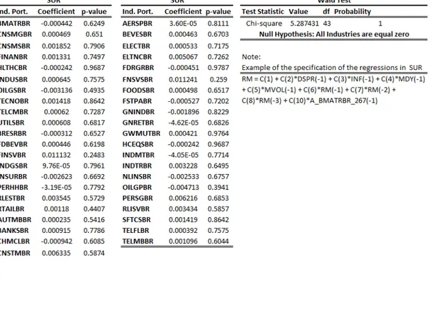
In Table7 a SUR is estimated, the SUR is useful when the error terms are in fact correlated between the equations, the standard errors, and consequently the p-values take in account these correlations. The results show that all industries don’t have predictive power, the Wald-test have big p-values. Many configurations and industry levels were estimated, all with the same conclusions. I’ve excluded the subsectors data because they are multicolinear with the other industry portfolios.
Table 7: Seemingly Unrelated Regressions (SUR) estimated and Wald-test
There is no significant industry portfolio, the Wald-test confirm this hypothesis. This is a modification of Predictive regression 1.
20 Besides the SUR and the OLS, estimated in a system, in Table 8 I’ve estimated regressions using all industries simultaneously in the same regression. To do this I’ve excluded some Industries portfolios, otherwise I would have multicolinearity problems. Like TSE I try some model configurations, the models with the Newey-West corrections have p-values (Wald-test) on the industries portfolios coefficients that are jointly significant, the models with no correction, with 3 lags of market returns doesn’t present significant industries portfolios coefficients. In all regression there are a small amount individually significant industries, this can also be seen in Table 8.
Table 8: Forecasting the market using industries simultaneously
The regressions with the Newey-West correction have coefficients that are jointly significant. In all regression there are individually significant industries. There are two industries portfolios, with NW correction of 3 lags and using only sector level data, which are significant at a 10% level.
21 6. Robustness analysis
To check whether our results hold for two sub-samples I create diagrams that compare the whole sample results with the sub-sample ones. I arbitrary split the data in two parts. The range is from August of 1994 to September of 2005 in the first sample and from October of 2005 to September of 2016 in the last one. Since there are industries that have less observations in the first sample I’ve excluded the series with doesn’t have all the months in both samples. Therefore this analysis will include 37 industries portfolios.
In Table 9 I investigate the models and regressions that test if industries lead the stock market hold results for two sub-samples. The first white columns (All sample) in the left of the Table 9 are the same as the white columns on Table 6, they represent the regressions that test if industries portfolios are leading indicators for the market return. The next two class of columns (1994 – 2005 and 2005 – 2016) in grey and white are the results of the leading industries portfolios regressions for the two sub-samples. The Significance level is 1% (***), 5% (**), 10% (*). The columns in grey called “Both 3 Samples” check if the models for the both three samples exhibit significant industries portfolios. If there is a “1” it means that, in both three samples, the model have a significant industry portfolio.
Table 10 investigates the models and regressions that test if industries lag the stock market and if this results hold for two sub-samples. The logic of the table is equal to the logic in Table 9.
Table 9 and Table 10 demonstrate that the results aren’t, in general, robust. The columns called “Both 3 Samples” don’t display a single industry portfolio that has more than one model with significant coefficients in both three samples. Of the “leading” industries portfolios of Table 6, only Utilities and Electricity have a single model that has significant coefficients in both three samples. Of the “lagging” industries portfolios of Table 6 only Commodity Chemicals have a single model that has significant coefficients in both three samples.
22
Table 9: Robustness analysis for the leading models
This Table investigates if the leading industries portfolios are robust to a sub-sample analysis. There isn’t an industry portfolio with more than a model with significant coefficients. Take as an example Auto & Parts, a leading industry portfolio if the whole sample is used, there isn’t a model where both three samples display significant coefficients. Only Utilities and Electricity have a model with significant coefficients in both three samples. If there is a “1” in the last nine columns “Both 3 Samples” it means that, in both three samples, the model have a significant industry portfolio.
23
Table 10: Robustness Analysis for the lagging models
This Table investigates if the lagging industries portfolios are robust to a sub-sample analysis. There isn’t an industry portfolio with more than a model with significant coefficients. Take as an example Speciality Fin, a lagging industry portfolio if the whole sample is used, there isn’t a model where both three samples display significant coefficients. Only Commodity Chemicals have a model with significant coefficients in both three samples. If there is a “1” in the last nine columns “Both 3 Samples” it means that, in both three samples, the model have a significant industry portfolio.
24 7. Conclusions
The main purpose of this paper is to investigate the causality between the market and industries for Brazil. HTV investigated only the causality from the industries to market and say nothing on the causality from market to industries. TSE realized that, to claim causality one has to test both directions. For Brazil, I conclude that isn’t possible to claim causality from industries to the market. Table 4 illustrate this, it’s not clear that industries lead stock markets in Brazil, because using the same scope of tools that HTV, I have the same evidence from market to industries, there is as much as the same amount of valid coefficients with market as exogenous variable, industries as endogenous and the opposite.
To check if there are leading or lagging industries independent of the specification of the model, I have constructed Table 6, it’s possible to find some leading and lagging industries, when deepening the analysis, in Table 9 and in Table 10, to check for robustness, the results are less significant. Utilities and Electricity appear to be leading industries and only Commodity Chemicals appear to be a lagging industry portfolio.
In Table 5 it’s possible to see that lagged IPG explains industries returns more than the reverse, proportionally. IPG has a clear correlation with market return and in Figure 2 this relationship is more evident. This can be seen as an evidence of contemporaneous relationship between IPG and market return. In this case the economic information is absorbed by the market participants and, consequently, the market return, during the same month. However is worth to note that if there is gradual diffusion from the market to industries this would be evident in this analysis, there is no strong evidence of significant lagging models where industries are endogenous and lagged market return is exogenous. This can be seen as evidence that IPG and market return aren’t leading indicators for industries portfolios in Brazil. Besides the evidence, a proper causality test between IPG and industries portfolios (individually) follow as a suggestion for a next study.
The SUR estimated in a system, doesn’t present individually significant industries portfolios coefficients, a Wald-test confirm the insignificance of the coefficients jointly tested, this show that if the contemporaneous correlation between the industries portfolios is somehow taken into account there is no gradual diffusion of information from the industries to the market. The Wald-test on the OLS estimated in a system reject the joint significance of the industries portfolios. Other possibilities are that the volatility of the Brazilian variables (which are higher than in any of the HTV countries) or the validity of the controls variables chosen, invalidate the models estimated in a system, although I’ve tested many model specifications. Since there is no consensus when estimating systems with the same endogenous variables, those are secondary results.
HTV, extending the analysis to the rest of the world, found significant F-statistics, when estimating regressions with exogenous lagged industries portfolios simultaneously. TSE using an updated sample, only found one model with significant F-statistics, but this model present only a few or none, depending on the significance level, relevant lagged industries portfolios coefficients. In Table 8 I have estimated regression with exogenous lagged industries portfolios simultaneously. I found some models with jointly significant coefficients, but with a small amount on individually significant coefficients.
25 References
Campbell, John Y. and Robert J. Shiller, 1988, “The dividend-price ratio and expectations of future dividends and discount factors,” Review of Financial Studies 1, 195- 228.
Fama, Eugene and G. William Schwert, 1977, “Asset returns and inflation,” Journal of Financial Economics 5, 115-146.
Fama, Eugene and Kenneth French, 1989, “Business conditions and expected returns on stocks and bonds,” Journal of Financial Economics 25, 23-49.
Fiske, Susan and Shelley Taylor, 1991, Social Cognition 2nd ed., McGraw-Hill, New
York.
Hong, Harris, Torous, Walter and Valkanok, Rossen, 2004 “Do Industries Lead Stock Markets?”.
Hong, Harrison and Jeremy C. Stein, 1999, “A unified theory of underreaction, momentum trading and overreaction in asset markets,” Journal of Finance 54, 2143-2184.
Industry Classification Benchmark, Industry Structure and Definitions Website. < http://www.icbenchmark.com/ICBDocs/Structure_Defs_English.pdf >
Kahneman, Daniel, 1973, Attention and Effort (Prenctice-Hall, Englewood Cliffs, New Jersey).
Lamont, Owen, 2001, “Economic tracking portfolios,” Journal of Econometrics 105, 161-184.
Merton, Robert C., 1987, “A simple model of capital market equilibrium with incomplete information,” Journal of Finance 42, 483-510.
Nisbett, Richard and Lee Ross, 1980, Human Inference: Strategies and Shortcomings of Social Judgment (Prentice-Hall, Englewood Cliffs, NJ).
Shiller, Robert J., 2000, Irrational Exuberance, (Broadway Books: New York).
Sims, Christopher, 2001, “Rational Inattention,” Princeton University Working Paper. Torous, Walter, Ross Valkanov, and Shu Yan, 2004, “On predicting stock returns with nearly integrated explanatory variables,” Journal of Business 77, 937-966.
Tse Yuman, 2015, “Do industries lead stock markets? A reexamination” Journal of Empirical Finance 34, 195-203.
Valkanov, Rossen, 2003, “Long-horizon regressions: Theoretical results and applications,” Journal of Financial Economics 68, 201-232.