www.scielo.br/rbg
DIFFICULTIES ASSOCIATED TO THE ULTRASONIC IMAGING OF SMALL SCALE MODELS
OF STRATIGRAPHIC DEPOSITS
C´assio Stein Moura
1, Roseane Marchezi Miss´agia
2and Marco Antonio Rodrigues Ceia
2ABSTRACT.Mechanical waves are commonly used on the characterization of geological systems. Highly compacted real systems require low frequency waves on the order of tens of hertz. Tabletop models span the millimetric scale and therefore need higher frequency waves ranging up to the ultrasound band. We have used an ultrasonic seismic equipment to image tabletop geological systems. The seismograms enabled the identification of some features under investigation but were limited to discern some objects of interest, such as, the interface between a coal layer on top of a sand layer. We believe that the low consolidation of the material has intensified the Rayleigh scattering of the incident wave leading to a large signal attenuation and to the difficulty on layer discrimination. We propose some ways to circumvent such a problem including increasing the material consolidation or the sediment grain size in order to reduce the scattering effects.
Keywords: mechanical waves, deposit imaging, stratigraphy, turbidity currents.
RESUMO.A utilizac¸˜ao de ondas mecˆanicas ´e uma opc¸˜ao recorrente na caracterizac¸˜ao de sistemas geol´ogicos. Sistemas reais de alta compactac¸˜ao costumam ser analisados por ondas mecˆanicas com frequˆencias da ordem de dezenas de hertz. Modelos de bancada requerem o uso de frequˆencias mais altas, na faixa do ultrassom, para possibilitar a definic¸˜ao de detalhes milim´etricos. Utilizamos um sistema de levantamento s´ısmico ultrassonogr´afico para visualizar modelos geol´ogicos de bancada. Os sismogramas produzidos identificaram algumas feic¸˜oes sob investigac¸˜ao, mas apresentaram limitac¸ ˜oes na discriminac¸˜ao dos objetos de interesse, a saber, a interface entre uma camada de carv˜ao sobre uma camada de areia. Acreditamos que a baixa consolidac¸˜ao do material tenha intensificado o espalhamento Rayleigh da onda incidente levando a uma grande atenuac¸˜ao do sinal de retorno e `a consequente dificuldade em discriminar as camadas. Propomos algumas formas de diminuir esse problema que incluem o aumento da consolidac¸˜ao do material ou do tamanho de gr˜ao dos sedimentos para reduzir os efeitos de espalhamento.
Palavras-chave: ondas mecˆanicas, visualizac¸˜ao de dep´ositos, estratigrafia, correntes de turbidez.
1Faculdade de F´ısica, Pontif´ıcia Universidade Cat´olica do Rio Grande do Sul, Av. Ipiranga, 6681, 90619-900 Porto Alegre, RS, Brazil. Phone: +55(51) 3353-7838; Fax: +55(51) 3320-3616 – E-mail: [email protected]
2Laborat´orio de Engenharia e Explorac¸˜ao de Petroleo, Universidade Estadual do Norte Fluminense Darcy Ribeiro, Rodovia Amaral Peixoto, km 163, Av. Brennand s/n, Imboacica, 27925-535 Maca´e, RJ, Brazil. Phones: +55(22) 2765-6564, +55(22) 2773-8032; Fax: +55(22) 2765-6565 – E-mail.: [email protected]
INTRODUCTION
Turbidity currents are defined as a gravitational flow of sedi-ments in water under the influence of a differential thrust due to the density difference in the environment. They are rare and un-foreseeable events making their observation quite difficult. They have strong social consequences for they usually occur on the Brazilian mountain slopes impacting the life of thousands of peo-ple and implying huge economic losses. Turbidity currents also occur in the subsea environment leading to debris accumula-tion at deep-water regions which are called turbidites (Middle-ton, 1993; Stelting, 2000; Peakall et al., 2001). In such a case, the phenomenon may be related to the existence of oil reservoirs. Roughly one third of the world hydrocarbon reservoirs happen on turbidite deposits (Manica, 2002). Therefore, understanding turbidity flows presents great economic interest as well as a defy-ing basic science subject. Due to the difficulties associated with real time observations on the nature, this kind of phenomenon is usually simulated in laboratory at small scale.
The physical simulation of small scale systems is very com-mon in geology because it allows to alter the time scale and the required room space and, inasmuch as, it allows the understand-ing of the real natural system evolution (Schneider, 1998; Salvi et al., 2011; Ramirez et al., 2013). Since large volumes of fluid and sediments are required for the simulations, only a few labo-ratories in the world are able to run this kind of experiment. In order to compensate this difficulty, computer simulation has been used to study density currents. There is still a lack of classifica-tions and physical understanding of all related phenomena which involve the interaction between the flux and the seabed as well as the presence of several different types of substances.
Despite all efforts on understanding the formation of density currents there is still a great deal of work to be done. In their review article Wynn et al. (2007) state that deposits of subma-rine channels are yet not well understood and show great deal of differences among each other. In order to overcome this kind of difficulty, several authors proposed the study of turbidity cur-rents and their effects using small scale models. In their re-view article, Paola et al. (2009) discuss the reasonableness of comparing small scale physical models of channel systems and systems under pluvial erosion to natural systems. They present several physical simulations results obtained by themselves and others who used photogrametry and laser scanning to map de-posits surfaces. These techniques allows only the system sur-face imaging but not its interior. Other authors likewise used laser scanning to obtain the topography of small scale physi-cal models (Strong, 2006; Martin, 2007; Gerber et al., 2008).
Ashmore et al. (2001) employed a constant discharge into a 54 m2tank in order to simulate braided rivers and observed that
despite the incorporation of very simple assumptions on grain size distribution and lateral water surface the predictions are quite reasonable when compared to a real river. Their conclu-sions were based on the study of digital photogrametry per-formed at regular intervals of time. Kane et al. (2010) simulated the submarine channels to understand the influence of the flow on their levees. The system consisted of a 4.3 m3tank with a curved
channel in which a flow of glass micro spheres and ground silica mixed in tap water was thrown. Successive runs were performed and in between each run, the surface was mapped with ultrasonic bathymetry allowing the observation of the deposit evolution. It was possible to relate the overflow characteristics to the ero-sion regime and the accretion on the channel levees. No inte-rior imaging was performed. Cartigny (2012) studied the chan-nel dynamics and structure formation using a narrow straight tank with a length of 12 m. The tank walls were made of glass in order to permit a direct observation of the sedimentation. A photographic camera was used to acquire the images. This kind of experiment provides only the one-dimensional behavior of the depositional system. Literature presents several works similar to the ones cited above but in a general way the experiment is not able to visualize the inner parts of the sediments, for those imaging techniques are based on the reflection of light or sound waves on the top or lateral surfaces of the deposit.
Manica (2002) simulated non-conservative density currents in two- and three-dimensional channels using sand, coal and limestone. In his experiments the sediment is mixed in tap wa-ter which is launched into a channel ending up in a basin where a small scale delta is formed. Variation of several parameters such as type of sediment, grainsize and concentration, turns possible to produce different forms of the flow at the channel mouth. Del Rey (2006) used this same technique to simulate a turbidite flow on the east Brazilian continental margin and identi-fied new geometric and dynamic aspects of the non-conservative density currents and their consequences on the sedimentation. However, as discussed above, the development of such physi-cal simulations is barred by the same difficulty: visualizing the inner stratigraphic layers formed during deposition. The pro-cedure used to image the deposit interior employed by Man-ica (2002) and Del Rey (2006) starts with the full tank drain-ing and sediment drydrain-ing, followed by the deposit complete slic-ing. Each cutting plane is dried and subsequently photographed. The whole process is time consuming, destroys the whole sam-ple and, moreover, provides images of a system which was
rearranged during the drainage process and therefore is just an approximation of the initial colloidal system formed during the depositional stage. It is necessary to develop new ways to effi-ciently visualize the internal structures of the deposits on a non-invasive fashion.
Low frequency mechanical waves are frequently used to characterize real geological systems which points to the pos-sibility of using them on small scale systems characterization. Due to the small dimensions of the employed models a high fre-quency wave is needed in order to produce a reasonable resolution of the depositional system. In this work we adapt the large scale seismic technique to a small scale bench top model. In order to do that we used the ultrasonic part of the sound spectrum. We look for details on the millimeter range which requires frequen-cies above 100 kHz. In this technique a transducer emits a short pulse of 1 ms duration. Another transducer is placed sideways with zero offset and waits for the returning echoes originated at the surfaces of the sample under study. The maximum waiting time is defined at about 1 s. In order to decrease the signal to noise ratio the emission and reception process is repeated sev-eral times for the same transducer position. We call each one of this processes a shot. After a predetermined number of shots is reach for a specific position the transducer pair is displaced laterally and a new shot sequence is initiated. The transducer set displacement follows a straight line on the model surface. At every interface within the sample, in which there is a change on the acoustic impedance, the signal is reflected and a phase inver-sion may take place. The depth at which the reflection happened is calculated through the observed signal transit time and the sound velocity, that must be known beforehand. For each shoot-ing line the reflections depths are determined and the seismo-gram is obtained.
METHODOLOGY Model preparation
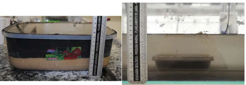
Two synthetic models were built inside plastic boxes of differ-ent sizes. The larger model was 20 cm wide and the smaller one was 10 cm wide. From now on, we will call them model 1 and model 2, respectively. Sand and coal are two types of materials that are regularly used in small scale simulations because they have good optical contrast. Moreover, since their density ratio is roughly 2 and the sound velocity differs by about 20% their acoustic impedance should be sufficiently different to produce reflections on the interface between both substances. Therefore, these substances seem adequate to be used with the echographic technique. Since the specific mass is greater for sand than coal,
sand was placed at the bottom of the deposit and coal at the top position, minimizing the possibility of mixing both substances during sample handling. The used materials were cardiff coal (Rio Deserto, Crici´uma, Santa Catarina State, Brazil) and fine-grained construction sand. The model was built on the following way. Water was poured into the plastic box, followed by the sand which was placed very carefully in order to obtain a homogenous distri-bution. Afterward, the surface was smoothed. The system was let to rest for one hour allowing sand full sedimentation. The coal was meticulously placed on top of the sand. Adding water to the model ahead of the sediments provides a good sonic coupling allowing the mechanical waves propagation towards the bottom. In model 1, each sand and coal layer was 4 cm height. In model 2, these layers were 1 and 2 cm, respectively. The measurements were performed in two configurations:
i) only a small water depth on top of the model and no water surrounding it;
ii) the model placed within a glass tank with a variable water level, but always above the model.
In case ii) the tank was filled with water in a slow way in order to not disturb the synthetically created structure. The choice of using a model smaller than the tank allows the identification of the glass bottom in the regions outside the model but within the tank, improving seismic interpretation. Figure 1 shows the final aspect of each model.
Description of the measurement instrument
The seismic survey instrument used in this work is located at the Reservoir Integrated Modeling Laboratory at LENEP/UENF, Maca´e, Rio de Janeiro State. It comprises two ultrasonic im-mersion transducers that can be moved over a horizontal plane through a stepping motor system. The transducers are vertically oriented, parallel to each other and their offset is adjustable. In our work we used a zero offset in order to guarantee normal inci-dence and reflexion at the surface. One transducer plays the role of emitter and the other one is the receiver. More equipment details such as pulse waveform, frequency spectrum and signal length are given by Miss´agia et al. (2010). In our experiment, the transducers were moved over a horizontal line on the water sur-face while the signal was emitted and acquired by the transducers aiming at the coal/sand interface identification. Frequencies were set at 250, 500 and 1000 kHz, voltages ranged from 10 to 70 V and 100 to 500 shots were stacked for each position. The trans-ducers were kept in contact with the water surface to guarantee acoustic coupling.
Figure 1 – Final aspect of the models. Model 1 (left) and model 2 (right). Model 2 is shown immersed in the water filled tank. In the upper right corner one can see
the ultrasonic transducers. Note the zero offset of the transducers.
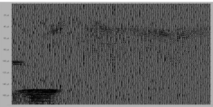
Figure 2 – Seismogram of model 1 using the parameters: 100 shots per step, frequency of 250 kHz and 10 V applied to the transducer. At the upper left corner the
rectangle represents 1 cm on the horizontal direction. The water/coal interface is indicated by the horizontal white bar and spread over the whole seismogram width.
RESULTS
The initial trials were made with model 1 having a water depth of 1 cm over the coal surface. The transducer were moved over a straight line within the inner edges of the plastic box which con-tains the model; frequencies of 250 and 500 kHz were used and 100 shots per position were stacked. The resulting seismogram allowed the identification of the water/coal surface but did not allow the identification of the coal/sand interface. In Figure 2 we show the resulting seismogram using a 250 kHz frequency. This image can be understood as a seismic section of zero offset. No numerical processing was performed on the data.
Facing the difficult task of interpreting this seismogram, we decided to make use of markers to allow for a comparing scale near the model. The model was placed in the tank which was
filled with water up to the level of 2 cm above the top of the coal surface. With this new geometry, the transducers are able to move not only within the edges of the plastic box but be-yond them. We hoped that with this new configuration it would be possible to identify the bottom glass surface of the tank which in turn could indicate the sand/plastic bottom of the model. At the external left side of the model a marker was placed. It was made of a plastic cylinder filled with sand and with known di-mensions (4× 1 cm). The drawing in Figure 3 shows the model submersed in water and the marker on its side. In the image the transducers are at their initial position and during the data acqui-sition they will move to the right side.
Obviously, the scale provided by the cylinder allows a di-rect reading just outside the model which is a region containing
Figure 3 – Drawing of the experimental set up. The transducers are at their initial
position and will move to the right. A marker is placed outside the model.
Figure 4 – Seismogram of model 1 using the parameters: 200 shots per step, frequency of 500 kHz and 10 V applied to the transducer.
The image has not undergone any numerical processing.
only water where the sound velocity is 1,483 m/s (Nussenzveig, 2002). Within the model, the scale must be converted taking into account another velocity. Tono (2007) observed that the sound velocity in ground wet coal is 1,834 m/s regardless the concen-tration of water with respect to carbon. Assuming this given ve-locity, one can calculate the position in the seismogram where the interface coal/sand should be at. In Figure 4, we show the seismogram for the situation when the model was placed in the tank with the water level above the plastic box and the marker serving as a scale outside the box. The seismogram interpreta-tion is shown in Figure 5. The transducers movement started at the left side and ended at the right side. The initial (left) part of the run clearly shows the bottom of the tank and the top of the marker. Going to the right, the transducers pass over the marker,
which can be seen as well, and eventually reach the model edge. At this point, diffraction hyperbolas are visible and are labeled in the figure asmodel edge. As the transducers follow their path over the model the seismogram shows the presence of the wa-ter/coal surface. However, the model inner structure (coal/sand interface) is not clearly identifiable. The transducers continue their movement beyond the other side of the model although this part of the seismogram is not shown in the figure for the right side is symmetrical to the left side. The calculated position of the coal/sand interface is shown in Figure 5 by the white horizon-tal line, despite the fact we could not clearly identify a reflector plane at this depth. The model bottom sand/plastic surface was not noticeable either. The lack of reflectors in the seismogram is probably due to the intense signal attenuation in the coal layer.
Figure 5 – Interpretation of the seismogram of model 1 shown in Figure 4. The white horizontal line shows the calculated position for the
coal/sand interface. At the upper left corner the rectangle represents 1 cm on the horizontal direction.
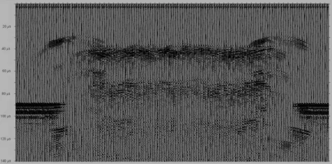
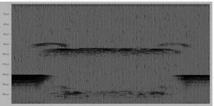
Figure 6 – Seismogram of model 2 using the parameters: 500 shots per step, frequency of 500 kHz and 50 V applied to the transducer.
In this experiment, coal is not consolidated, favoring the scatter-ing of the incident wave on several directions and decreasscatter-ing the part of the initial beam that returns to the acquiring transducer.
Aiming at the reduction of the signal attenuation by the coal we decided to sharpen the coal layer in the model. We built the model 2 in which the coal layer has half the thickness as model 1. The new model was placed in the tank and water was slowly poured in, up to the point where the water depth over the coal layer was 2 cm. We also increased the transducer voltage to 50 V in order to increase the signal intensity and improve the signal to noise ratio. Figure 6 shows the resulting seismogram without any numerical treatment and Figure 7 shows our interpretation.
Some structures that were already observed in model 1 (Figs. 4 and 5) show up again in model 2 such as the reflection at the bottom of the tank outside the model, the sound wave diffraction at the model edge and the reflection at the coal surface. More-over, some new almost horizontal lines appeared and could seem at a first sight as due to the coal/sand interface, after all, they are above (shorter transit time) the bottom surface of the tank out-side the model. These new features could as well be resulting from the reflections at the bottom of the model at the sand/plastic and plastic/glass surfaces. This assumption seems reasonable for the new horizontal lines have a shorter transit time than the re-flections outside the model. In addition, sound propagates faster
Figure 7 – Interpretation of the seismogram shown in Figure 5. At the upper left corner the rectangle represents 1 cm on the horizontal direction.
in coal and sand than in water. Nevertheless, some similar but less intense reflectors appeared at even deeper positions, seem-ing to be produced bellow the bottom of the tank! Thereupon, we wondered whether they could be reverberation artifacts. Sup-porting this suspicion are the less intense stacked hyperbolas that should be resulting from the wave diffraction at the model edge. It is interesting to discuss somewhat the concept of rever-beration artifacts applied to our case study.
A sound wave emitted by the transducer towards the model is reflected back to the receptor at each discontinuity on the acoustic impedance value. The first reflection in our case hap-pens at the water/coal surface for they have different acoustic impedances. When the reflection takes place, a refraction also occurs and the signal penetrates deeper into the sample being reflected and refracted again at the next discontinuity, e.g., the coal/sand surface. From the initial signal, a fraction returns to-ward the detector right after the first reflection whilst a consider-able parcel is scattered to other directions away from the trans-ducer. The scattered parcel reaches the water surface and encoun-ters the water/air discontinuity implying on a new reflection to-wards the model. After being reflected twice and moving to the coal surface once more it is eventually reflected back to the re-flector. It is worth saying that this mechanism may go on in-definitely but at each reflection the signal loses a considerable fraction of its intensity. After a sequence of reflections the sig-nal eventually reaches the detector and may be misinterpreted as a water/coal reflection surface at a deeper position. When sev-eral reflections occur the phenomenon is usually called ringing. The identification of reverberation artifacts is a procedure that in our case is easy to carry out: it suffices to increase the
wa-ter depth above the model and observe if the signal transit time increases correspondingly.
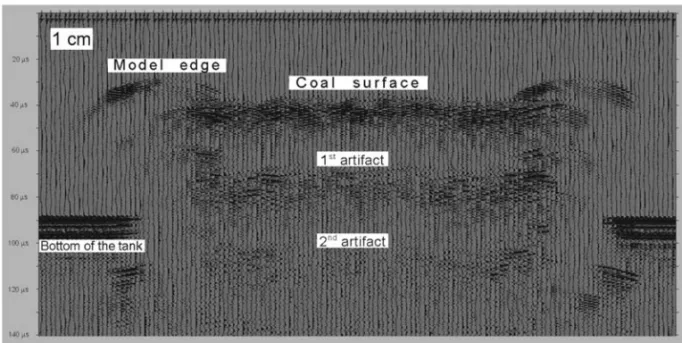
We increased the water depth and surveyed the model once more. Figure 8 shows the raw seismogram and Figure 9 rep-resents our interpretation. It is not hard to see that the second group of apparent reflectors suffered a displacement to a deeper position which evince the reverberation nature of these features. They are simply artifacts and do not represent a real reflector. Taking the above reasoning into account, and comparing Fig-ure 8(9) to FigFig-ure 6(7) it is ready to observe that in FigFig-ure 6(7) there are two reverberation artifacts (labeled1st and2ndartifact)
whilst in Figure 8(9) only the 1st artifact is clearly visible and at
a deeper position than the previous image.
Besides, there are nevertheless some minor differences among Figures 6(7) and 8(9). The increase on the water depth displaces the transit time of the reflection on the coal surface from 38 to 87 microseconds agreeing with the notion of a now deeper model. Figure 6(7) presents a higher amount of details because we stacked 500 shots per step instead of the 200 shots per step on Figure 8(9), altering the signal to noise ratio. Unfor-tunately the coal/sand interface was not identifiable in neither of the cases but only a diffuse scattering region. We performed sur-veys at the frequencies of 100, 250 and 1000 kHz, but obtained similar responses. Increasing the voltage to the instrument limit, e.g. 70 V, did not improve the layers discrimination.
DISCUSSION
We have made several attempts in order to distinguish a coal/sand reflecting surface in a bench top synthetic deposition model. Frequencies on the range of several hundreds of hertz
Figure 8 – Seismogram of model 2 using the parameters: 200 shots per step, frequency of 500 kHz and 50 V applied to the transducer.
Figure 9 – Interpretation of the seismogram shown in Figure 8. At the upper left corner the rectangle represents 1 cm on the horizontal direction.
were tested, hundreds of shots per step were stacked and several tens of volts were applied to the emitting ultrasonic transducer. Structures of consolidated materials such as the plastic box and the bottom of the tank outside the model were clearly detected and showed good agreement on their depth to the calculation based on the propagation velocity. However, the aimed interface signal, e.g. the coal/sand discontinuity, was not identifiable even when the upper layer was narrowed by half its thickness. Neither the bottom of the tank underneath the sample was identifiable. It was visible only outside the model box. The lacking bottom structure indicates that the sound wave is either not reaching the deepest parts of the model or not being able to make its way back to the
surface and consequently the detector. This indicates that a strong signal attenuation may be happening.
The ultrasonographic technique usually assumes a specular wave reflection at the acoustic impedance discontinuities in order to produce the structure image. This kind of reflection only occurs when the surface is very smooth and the same rules applied to the optical phenomena succeed. In the event of a rough surface, where the undulations typical sizes are similar to the incoming wavelength the reflected beam may be scattered to a wide solid angle, decreasing the returning signal detected by the transducer. Nevertheless, we were very careful during the sample preparation stage in order to assure the surface was as smooth as possible
in order to avoid this kind of effect and therefore assume that this effect should be minimal. On the other hand, when the traveling sound wave reaches a structure whose dimension is much smaller than the wavelength it is absorbed and irradiated in every direction following an isotropic distribution (Farr & Alissy-Roberts, 1998). In this case, only a small part of the initial signal returns to the detector, its intensity following an inverse square power law on the depth. The scattering of the incident wave by particles much smaller than the incident wavelength is known as Rayleigh scat-tering and, for example, explain the blue color of the Earth’s atmo-sphere. The theory used to describe electromagnetic waves can be adapted to explain mechanical waves scattering.
Considering the frequencies we used in this work and the propagation velocities cited above it is straightforward to calcu-late the used wavelength range: from 1.8 to 7.3 mm. The aver-age grain size of the used coal was of the order of 0.05 mm. It is reasonable then to assume that the wavelength is much larger than the average structural dimensions and scattering is playing an important role on the experiment. During the sample prepara-tion stage, sand and coal were simply poured into the container not having suffered any kind of extra compaction which in turn leaded to a low consolidation system. This fact could have played an important role on the scattering effect. If, on the other hand, the material had been extremely compacted, as it occurs to sedimen-tary rocks, the coal grains would have suffered an agglomeration process which would increase its average size, possibly reaching dimensions superior to the incoming beam wavelength. In such a case, the Rayleigh scattering would probably be reduced allowing an almost specular reflection on the acoustic impedance discon-tinuities evincing the aimed interface.
This initial trial to visualize the internal deposits structure through echography indicated the necessity of alterations on the instrumentation and sample preparation routines that shall be im-plemented in future works. One possible solution could be the use of a highly compacted model that could be obtained by a longer resting time between model preparation and data acquisition or the use of an external pressure to play the role of the natural sed-imentary rock formation process. The models used in this work were let resting and will be analyzed later. Surveys will be taken at regular time intervals in order to follow the consolidation stage.
A model that have been drained and dried having a thick-ness of the order of one meter (the typical thickthick-ness used by Manica and Del Rey) should present a higher compaction de-gree which should decrease signal scattering. However, despite a supposed improvement in visualization, the drainage process does not preserves the colloidal suspension obtained in
simula-tion tanks which in turn affects the interpretasimula-tion of the deposit formation process.
A possible solution would be substitute the simulation sub-stances by some material that reaches a higher compaction state or one that presents a larger grain size whilst preserving the nec-essary hydraulic properties to keep the scale factor unchanged providing small scale simulations that represent the natural large scale phenomena. This option requires a deep investigation on the synthesis of new materials.
CONCLUSION
Characterization of depositional systems can be done through the use of mechanical waves such as the known seismic survey methods. Small scale models require the use of frequencies on the ultrasound range to allow acceptable resolution images. The echographic technique proved to be adequate to identify some structures under investigation but showed to be limited in the discrimination of the objects of interest. The materials used as sediments did not permitted distinguishing the aimed reflecting interfaces. This fact seems to be caused by the isotropic scatter-ing of the incident wave due to the low consolidated state of the model which leads to a strong signal attenuation. In this work we discussed some possible solutions to overcome such a problem, including an increase in the resting time of the sediments, the use of an external pressure to increase the compaction state, an al-teration on the transducers geometry and the substitution of the simulation materials.
ACKNOWLEDGMENTS
The authors are greatly thankful to Petrobras for its financial support in this investigation effort as well as the permission to publish the results.
REFERENCES
ASHMORE P, BERTOLDI E & GARDNER JT. 2011. Active width of gravel-bed braided rivers. Earth Surface Processes and Landforms, 36: 1510–1521.
CARTIGNY MJB. 2012. Morphodynamics of supercritical high-density turbidity currents (Doctoral Thesis) – Faculty of Geosciences, Depart-ment of Earth Sciences, Utrecht University. 153 pp.
DEL REY AC. 2006. Simulac¸˜ao F´ısica de Processos Gravitacionais Subaquosos: uma aproximac¸˜ao para o entendimento da sedimentac¸˜ao marinha profunda. Thesis (Doctor of Geosciences) – Graduate Pro-gram on Geosciences, Institute of Geosciences, Federal University of Rio Grande do Sul. 229 pp.
FARR RF & ALLISY-ROBERTS PJ. 1998. Physics for Medical Imaging. Saunders: London. 196 pp.
GERBER TP, PRATSON LF, WOLINSKY MA, STEEL R, MOHR J, SWEN-SON JB & PAOLA C. 2008. Clinoform Progradation by Turbidity Cur-rents: Modeling and Experiments. Journal of Sedimentary Research, 78(3): 220–238.
KANE IA, McCAFFREY WD, PEAKALL J & KNELLER BC. 2010. Sub-marine channel levee shape and sediment waves from physical experi-ments. Sedimentary Geology, 223(1-2): 75–85.
MANICA R. 2002. Modelagem F´ısica de Correntes de Densidade N˜ao Conservativas em Canal Tridimensional de Geometria Simplificada. Dissertation (Masters of Engineering ) – Graduate Program in Engineer-ing and Water Resources, Institute of Hydraulic Research, Federal Uni-versity of Rio Grande do Sul. 122 pp.
MARTIN JM. 2007. Quantitative Sequence Stratigraphy (Philosophy Doctorate) Graduate School, University of Minnesota. 205 pp. MIDDLETON GM. 1993. Sediment Deposition from Turbidity Currents. Annu. Rev. Earth Planet Sci. 1993. 21: 89–114.
MISS´AGIA RM, CEIA M & PESSANHA CA. 2010. Modelagem F´ısica S´ısmica na UENF/LENEP: descric¸˜ao e teste do sistema. In: IV Simp´osio Brasileiro da SBGf, 2010, Bras´ılia. Proceedings. Bras´ılia: SBGf, 2010. CD-ROM.
NUSSENZVEIG HM. 2002. Curso de F´ısica B´asica, v. 2, Edggard Bl¨ucher: S˜ao Paulo, 314 pp.
PAOLA C, STRAUB K, MOHRIG D & REINHARDT L. 2009. The “un-reasonable effectiveness” of stratigraphic and geomorphic experiments. Earth-Science Reviews, 97: 1-43.
PEAKALL J, F´ELIX M, McCAFFREY B & KNELLER B. 2001. Particulate Gravity Currents: Perspectives. Spec. Publs. Int Ass. Sediment, 31: 1–8.
RAMIREZ JM, EGGENHUISEN J & CARTIGNY M. 2013. Effects of Gradual Increment of Clay Concentration on Turbidity Flow Structure. In: AAPG International Conference and Exhibition, Abstracts Volume, Cartagena: AAPG, 2013. CD-ROM.
SALVI F, CAPPELLETTI A, MEDA M, TESTI D, CAVOZZI C, NESTOLA Y, CHOWDHURY B, ARGNANI A, TSIKALAS F, MAGISTRONI C, DALLA S, ROVERI M & BEVILACQUA N. 2011. Integration of Sandbox Ana-logue Modeling and 2-D Structural Restoration as a Supplementary Tool to Exploration: Case Histories in Extensional, Transcurrent and Com-pressional Settings. In: AAPG International Conference and Exhibition, Abstracts Volume, Milan: AAPG, 2011. CD-ROM.
SCHNEIDER D. 1998. Tectonics in a Sandbox. Scientific American, 1: 36.
STELTING CE, BOUMA AH & STONE CG. 2000. Fine-Grained Turbidite Systems: Overview, In: BOUMA AH & STONE CG (Eds.), Fine-grained turbidite systems, AAPG Memoir 72/SEPM Special Publication, 2000. 1–8.
STRONG N. 2006. Mass Balance Effects in Clastic Fluvial Stratigra-phy (Doctor of PhilosoStratigra-phy) Graduate School, University of Minnesota. 125 pp.
TONO H. 2007. Phantom Seismic Stratigraphy: The origins of time-line reflectors and missing base-level markers from images and properties of experimental strata. Thesis (Doctor of Philosophy) Earth and Ocean Sciences Department, Nicholas School of the Environment, Duke Uni-versity. 119 pp.
WYNN RB, CRONIN BT & PEAKALL J. 2007. Sinuous deep-water chan-nels: Genesis, geometry and architecture. Marine and Petroleum Geol-ogy, 24: 341–387.
Recebido em 09 abril, 2012 / Aceito em 25 abril, 2013 Received on April 09, 2012 / Accepted on April 25, 2013
NOTES ABOUT THE AUTHORS
C´assio Stein Moura graduated in 1995 as a Bachelor in Physics and obtained his Masters degree in 1997 by the Federal University of Rio Grande do Sul, Brazil.
He is a Doctor of Science under the auspices of a collaboration project by the Federal University of Rio Grande do Sul and Penn State University, USA (2002). He is the Coordinator of the Geophysics course at the Pontifical University or Rio Grande do Sul. He has worked on magnetic properties of rocks, molecular dynamics simulation, ionic irradiation of intermetallics, nanostructures. He develops research on methods of non-invasive visualization of turbidite currents.
Roseane Marchezi Miss ´agia is a civil engineer (1985) by The Pontifical University of Minas Gerais, Master (1998) and Doctor (2003) on Reservoir Engineering
and Exploration, by the State University of Norte Fluminense Darcy Ribeiro (2003). She is a researcher at the State University of Norte Fluminense Darcy Ribeiro. She has published tens of papers in scientific journals and event annals; participated on the development of several technological products and received three awards. She works on the geoscience area with emphasis on applied geophysics. Interacts with several researchers as a coauthor in several scientific publications.
Marco Antonio Rodrigues de Ceia graduated in Physics at the Federal University of Rio de Janeiro (1994), Masters in Geophysics by the National Observatory
(1997) and Doctor of Reservoir and Exploratory Engineering by the State University of Norte Fluminense Darcy Ribeiro (2004). He is a professor at State University of Norte Fluminense Darcy Ribeiro. He has experience in the area of geoscience with emphasis on applied geophysics, working mainly in GPR, magnetometry and MT. He works on experimental research on petrophysics, rock physics and seismic physical modeling.