Dissertation
Masters in Computer Engineering – Mobile Computing
Optimization of Pattern Matching Algorithms
for Multi- and Many-Core Platforms
Pedro Miguel Marques Pereira
Dissertation
Masters in Computer Engineering – Mobile Computing
Optimization of Pattern Matching Algorithms
for Multi- and Many-Core Platforms
Pedro Miguel Marques Pereira
Master’s thesis carried out under the guidance of Professor Patrício Rodrigues Domingues, Professor at School of Technology and Management of the Polytechnic Institute of Leiria
and co-orientation of Professor Nuno Miguel Morais Rodrigues, Professor at School of Technology and Management of the Polytechnic Institute of Leiria and Professor Sérgio Manuel Maciel Faria, Professor at School of Technology and Management of the Polytechnic
Institute of Leiria.
Acknowledgement
I reserve this page to thank all whom supported me. My thanks go firstly to Professor Patrício Rodrigues Domingues for pulling me to this project and for his solid patience and availability. By extent, I thank adviser Professors Nuno M. M. Rodrigues and Professor Sérgio M. M. Faria for their project insight and patience over my uncertainties. I would like also to thank lab colleague Gilberto Jorge for filling in with his electronics knowledge whenever necessary. The contents of this dissertation would not be possible without any of them.
I also want to thank my family and girlfriend for letting me work after hours whenever it was needed without any concerns or preoccupations and for providing to my every need so that I could concentrate my daily life on this work. I also thank them for their predisposition and encouragement to see the end of this latest academic step.
Finally, I would like to thank the Escola Superior de Tecnologia e Gestão of the In-stituto Politécnico de Leiria and the InIn-stituto de Telecomunicações for the environment and working conditions that ultimately enabled this work. This work was supported by project IT/LA/P01131/2011, entitled “OPAC - Optimization of pattern-matching compression algorithms for GPU’s”, and financed by national Portuguese funds (PID-DAC) through Fundação para a Ciência e a Tecnologia / Ministério da Educação e Ciência (FCT/MEC), contract PEst-OE/EEI/LA008/2013.
Resumo
A compressão de imagem e vídeo desempenha um papel importante no mundo de hoje, permitindo o armazenamento e transmissão de grandes quantidade de conteúdos multimédia. No entanto, o processamento desta informação exige elevados recursos computacionais, pelo que a optimização do desempenho computacional dos algoritmos de compressão tem um papel muito importante.
O Multidimensional Multiscale Parser (MMP) é um algoritmo de compressão de padrões que permite comprimir conteúdos multimédia, nomeadamente imagens, al-cançando uma boa taxa de compressão enquanto mantém boa qualidade de imagem Rodrigues et al. [2008]. Porém, este algoritmo demora algum tempo para executar, em comparação com outros algoritmos existentes para o mesmo efeito. Assim sendo, duas implementações paralelas para GPUs foram propostas por Ribeiro [2016] e Silva [2015] em CUDA e OpenCL-GPU, respectivamente. Nesta dissertação, em complemento aos trabalhos referidos, são propostas duas versões paralelas que executam o algoritmo MMP em CPU: uma recorrendo ao OpenMP e outra convertendo a implementação OpenCL-GPU existente para OpenCL-CPU. As soluções propostas conseguem melho-rar o desempenho computacional do MMP em 3× e 2.7×, respectivamente.
O High Efficiency Video Coding (HEVC/H.265) é a norma mais recente para cod-ificação de vídeo 2D amplamente utilizado. Sendo por isso alvo de muitas adaptações, nomeadamente para o processamento de imagem/vídeo holoscópico (ou light field). Algumas das modificações propostas para codificar os novos conteúdos multimédia baseiam-se em compensações de disparidade baseadas em geometria (SS), desenvolvidas por Conti et al. [2014], e um módulo de Transformações Geométricas (GT), proposto por Monteiro et al. [2015]. Este algoritmo para compressão de imagens holoscópicas baseado no HEVC, apresenta uma implementação específica para pesquisar micro-imagens similares de uma maneira mais eficiente que a efetuada pelo HEVC mas a sua execução é consideravelmente mais lenta que o HEVC. Com o objetivo de possibilitar melhores tempos de execução, escolhemos o uso da API OpenCL como linguagem de programação para GPU de modo a aumentar o desempenho do módulo. Com a config-uração mais onerosa, reduzimos o tempo de execução do módulo GT de 6.9 dias para
pouco menos de 4 horas, atingindo efetivamente um aumento de desempenho de 45×.
Palavras-chave: computação de alto desempenho, Multi-Thread, Multi-CPU, Multi-GPU, OpenCL, OpenMP
Abstract
Image and video compression play a major role in the world today, allowing the storage and transmission of large multimedia content volumes. However, the processing of this information requires high computational resources, hence the improvement of the computational performance of these compression algorithms is very important.
The Multidimensional Multiscale Parser (MMP) is a pattern-matching-based com-pression algorithm for multimedia contents, namely images, achieving high comcom-pression ratios, maintaining good image quality, Rodrigues et al. [2008]. However, in comparison with other existing algorithms, this algorithm takes some time to execute. Therefore, two parallel implementations for GPUs were proposed by Ribeiro [2016] and Silva [2015] in CUDA and OpenCL-GPU, respectively. In this dissertation, to complement the referred work, we propose two parallel versions that run the MMP algorithm in CPU: one resorting to OpenMP and another that converts the existing OpenCL-GPU into OpenCL-CPU. The proposed solutions are able to improve the computational performance of MMP by 3× and 2.7×, respectively.
The High Efficiency Video Coding (HEVC/H.265) is the most recent standard for compression of image and video. Its impressive compression performance, makes it a target for many adaptations, particularly for holoscopic image/video processing (or light field). Some of the proposed modifications to encode this new multimedia content are based on geometry-based disparity compensations (SS), developed by Conti et al. [2014], and a Geometric Transformations (GT) module, proposed by Monteiro et al. [2015]. These compression algorithms for holoscopic images based on HEVC present an implementation of specific search for similar micro-images that is more efficient than the one performed by HEVC, but its implementation is considerably slower than HEVC. In order to enable better execution times, we choose to use the OpenCL API as the GPU enabling language in order to increase the module performance. With its most costly setting, we are able to reduce the GT module execution time from 6.9 days to less then 4 hours, effectively attaining a speedup of 45×.
Keywords: high performance computing, manycore, multi-CPU, multi-GPU, OpenCL, OpenMP
List of Figures
2.1 MMP Test Images . . . 11
2.2 HEVC Test Figure . . . 11
3.1 OpenMP Fork-Join Model . . . 24
3.2 MMP-Sequential encoder partial call-graph . . . 28
3.3 OpenMP Thread-Variation Effect over Jetson . . . 32
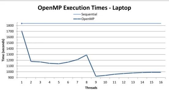
3.4 OpenMP Thread-Variation Effect over Laptop . . . 33
3.5 OpenMP Lambda-Variation Effect over Server 3 . . . 35
3.6 MMP-OpenMP mean watt oscillation over Jetson . . . 38
3.7 MMP-OpenMP mean watt oscillation over Server 2 . . . 39
3.8 Comparison between CPU and GPU Architecture . . . 41
3.9 Work distribution with SIMD instruction sets . . . 44
3.10 MMP-OpenCL mean watt oscillation over Server 2 . . . 48
3.11 MMP Rate-Distortion Curves . . . 50
4.1 GT 9 corner points . . . 53
4.3 HEVC+SS+GT sequential encoder partial call-graph . . . 58
4.4 HEVC+SS+GT-OpenCL K2 Visual Explanation . . . 73
List of Tables
2.1 Hardware Equipment Details - CPUs . . . 8
2.2 Hardware Equipment Details - GPUs . . . 9
2.3 Phoronix RamSpeed Test Results . . . 15
2.4 LZMA Benchmark Results . . . 16
2.5 PMBW Benchmark Results . . . 17
2.6 PMBW ScanRead64PtrUnrollLoop Benchmark Results - Access Time . 17 3.1 MMP-Sequential Results . . . 23
3.2 MMP-CUDA Results . . . 23
3.3 MMP-OpenCL-GPU Results . . . 24
3.4 MMP-OpenMP Results . . . 31
3.5 MMP-OpenMP Results with/without memory related problems . . . . 33
3.6 MMP-Sequential encoder with improvements . . . 34
3.7 Comparison between improved Sequential encoder and MMP-OpenMP . . . 34
3.8 OpenMP Energy Consumption Performance over Jetson . . . 38
3.10 Execution Time Evolution from OpenCL-GPU to CPU . . . 45
3.11 Kernel Time Evolution from OpenCL-GPU to CPU for the Laptop . . 47
3.12 OpenCL Energy Consumption Performance over Server 2 . . . 48
4.1 HEVC-Sequential Results . . . 60
4.2 HEVC+SS+GT-OpenMP Extremes . . . 62
4.3 HEVC+SS+GT-OpenMP Results . . . 63
4.4 HEVC+SS+GT-OpenCL clEnqueueCopyBuffer Time . . . 69
4.5 HEVC+SS+GT-OpenCL Kernel Copy Time . . . 69
4.6 HEVC+SS+GT-OpenCL N Iteration Simulations for N=2 . . . 70
4.7 HEVC+SS+GT-OpenCL Memory Used in GPU . . . 71
4.8 HEVC+SS+GT-OpenCL Kernel Execution Times . . . 80
List of Abbreviations
Abbreviation [A-I] Description
ALU Arithmetic Logic Unit
API Application Programming Interface
ARM Advanced RISC Machines
AVC Advanced Video Coding
AVX Advanced Vector Extensions
CD Compute Device
CPU Central Processing Unit
CSV Comma-Separated Values
CU Compute Unit
CUDA Compute Unified Device Architecture
D2D Device-to-Device
D2H Device-to-Host
DDR3 Double Data Rate, type Three
DDR3L Double Data Rate, type Three, LowVoltage
DFT Discrete Fourier Transforms
DIMM Dual Inline Memory Module
DSP Digital Signal Processor
ESTG School of Technology and Management (Escola Superior de Tecnologia e Gestão)
FCT Fundação para a Ciência e a Tecnologia
FFT Fast Fourier Transform
FP Floating Point
FPGA Field-Programmable Gate Array
FWHT Fast Walsh-Hadamard Transform
GCC GNU Compiler Collection
GPU Graphics Processing Unit
H2D Host-to-Device
HAD HEVC Walsh-Hadamard Transform
HDMI High-Definition Multimedia Interface
HEVC High Efficiency Video Coding
I/O Input/Output
IEC International Electrotechnical Commission
ILP Instruction Level Parallelism
IPL Instituto Politécnico de Leiria
Abbreviation [I-S] Description
ITU International Telecommunication Union
ITU-T ITU Telecommunication Standardization Sector
JCT-VC Joint Collaborative Team on Video Coding
L1 (cache) Level 1
L2 (cache) Level 2
LLC Last Level Cache
LP (Jetson mode) LowPower
MEC Ministério da Educação e Ciência
MF (Jetson mode) MaxFrequency
MIPS Million Instructions Per Second
MMP Multidimensional Multiscale Parser
MMP-OpenCL MMP OpenCL implementation
MMP-OpenCL-CPU MMP OpenCL implementation optimized for CPUs MMP-OpenCL-GPU MMP OpenCL implementation optimized for GPUs
MMP-OpenMP MMP OpenMP implementation
MP (Jetson mode) MaxPerformance
MPEG Moving Picture Experts Group
MPI Message Passing Interface
MSD Mean Squared Deviation
MSE Mean Square Error
NVCC NVidia CUDA Compiler
OpenCL Open Computing Language
OpenCL-CPU OpenCL optimized for CPU
OpenCL-GPU OpenCL optimized for GPU
OpenMP Open Multi-Processing
OS Operating System
PBM Portable BitMap graphics
PE Processing Element
PGAS Partitioned Global Address Space
PGM Portable GrayMap graphics — an alternatice to PBM
PIDDAC Programa de Investimentos e Despesas de Desenvolvimento da Administração Central
POSIX Portable Operating System Interface
PSNR Peak Signal-to-Noise Ratio
RAM Random-Access Memory
RISC Reduced Instruction Set Computer
RMS Root Mean Square
SIMD Single Instruction, Multiple Data
SMX Streaming Multiprocessor
SoC System on a Chip
SO-DIMM Small Outline Dual Inline Memory Module
Abbreviation [T-Z] Description
TLP Thread-Level Parallelism
µops micro-operations
USB Universal Serial Bus
VCEG Video Coding Experts Group (also know as Question 6 (Vi-sual coding) of Working Party 3 (Media coding) of Study Group 16 (Multimedia coding, systems and applications) of the ITU-T)
VMX Virtual Machine eXtensions
WHT Walsh-Hadamard Transform
WORA Write Once, Run Anywhere
Symbols Description
λ Ponderation factor of the relative weight of the distortion and the number of bits in the cost for a block representation expression
D Distortion caused by a block representation of the original image vs an element of the dictionary
J Cost for a block representation
R Number of necessary bits for a block representation
µ Micro
Index
Acknowledgement III
Resumo V
Abstract VII
List of Figures X
List of Tables XII
List of Abbreviations XIII
1 Introduction 1
1.1 Motivation . . . 2
1.2 Main Goals and Contributions . . . 3
1.2.1 Publications . . . 4
1.3 Outline . . . 5
2 Computational Environment and Methodology 7 2.1 Equipment and Configurations . . . 7
2.2 Results Acquisition and Used Images . . . 10
2.2.1 SpeedUp . . . 12
2.2.2 PSNR and Bitrate . . . 12
2.3 Energy Measurements Methodology . . . 13
2.4 Base Bandwidth Speeds . . . 14
3 MMP – Multi-CPU, Many-Core, Multi-Thread 19 3.1 Multidimensional Multiscale Parser . . . 20
3.2 Previous Versions . . . 21
3.2.1 MMP-CUDA and MMP-OpenCL-GPU . . . 21
3.2.2 Base Reference Results . . . 23
3.3 OpenMP . . . 24
3.3.1 Profiling MMP-Sequential . . . 26
3.3.2 Implementation . . . 30
3.3.3 Results . . . 31
3.4 OpenCL-CPU . . . 40
3.4.1 Migrating from OpenCL-GPU to OpenCL-CPU . . . 42
3.4.2 SIMD-based Optimizations . . . 43
3.4.3 Results . . . 45
3.5 Conclusions . . . 49
4 HEVC+SS+GT – Multi-GPU, Many-Core, Multi-Thread 51 4.1 High Efficiency Video Coding . . . 51
4.1.1 HEVC-based holoscopic coding using SS and GT compensations 52
4.2 Parallelization Impediments . . . 55
4.3 Profiling HEVC+SS+GT . . . 57
4.3.1 Base Reference Results . . . 60
4.4 OpenMP . . . 60 4.4.1 Implementation . . . 61 4.4.2 Results . . . 62 4.5 OpenCL-GPU . . . 63 4.5.1 Implementation . . . 64 4.5.2 Results . . . 79 4.6 OpenCL-Multi-GPU . . . 81 4.6.1 Implementation . . . 81 4.6.2 Results . . . 83 4.7 Conclusions . . . 84 5 Conclusions 85 Bibliography 87
Chapter 1
Introduction
The research presented in this dissertation relies on the optimization of an image compression algorithm, Multidimensional Multiscale Parser (MMP) [6, 7], that was recently parallelized to GPUs by Ribeiro [2] and Silva [3], resorting to both CUDA and OpenCL languages for GPU programming. To complement their work we further research and develop similar parallel implementations for multicore CPUs. One in OpenCL based on the existing implementation [3] but for CPU, and another resorting to OpenMP – a more CPU directed API – to provide result comparisons.
Afterwards, we decide to exploit our knowledge in the parallelization field to improve a specific algorithm based on the High Efficiency Video Coding (HEVC). This task consisted on the optimization of the recent HEVC-base implementation of Monteiro et al. [5] targeted to compress holoscopic image/video based on geometry-based dis-parity compensation (SS) and geometric transformations (GT) – henceforth referred as HEVC+SS+GT. This image compression algorithm has been chosen due to the emerging usage of plenoptic (or light field) images in various fields of application. The plenoptic function concept [8], represented by Equation 1.1, was introduced and developed by Adelson and Bergen and describes everything that can be seen (from plenus, complete or full, and optic). It embodies a way of thinking about light, not only as a series of images formed from 3D space onto 2D planes (whether retinal or cameras), but rather as a three-dimensional field of co-existing rays. This is a formalization of the concept of light-field proposed and coined by Gershun [9], with roots back to concepts introduced by Faraday [10] in the mid 19th century. Later, McMillan and Bishop [11] discuss the
representation of 5D light fields as a set of panoramic images at different 3D locations. The plenoptic function represents the intensity or chromacity of the light observed from every position and direction in 3-dimensional space. In image based modelling, the aim is to reconstruct the plenoptic function from a set of examples images. Once the plenoptic function has been reconstructed it is straightforward to generate images
by indexing the appropriate light rays. If the plenoptic function is only constructed for a single point in space then its dimensionality is reduced from 5 to 2. In the function Equation 1.1, the Vx, Vy and Vz variables are the possible viewing-points, and the x
and y variables parametrize the rays coordinates that are entering a given view-point (i.e. spatial coordinates of an imaginary picture plane erected at a unit distance from the eye pupil), for every wavelength λ, at every time t.
P = P (x, y, λ, t, Vx, Vy, Vz) (1.1)
Henceforth, this type of images presents much richer information than common 2D images, as they include information from several view directions, allowing to extract 3D information. However the computational complexity associated with its processing and compression may increase significantly. Therefore, for most applications it is imperative to reduce the algorithm execution time. To this end, we elected the use of the OpenCL API as the GPU enabling language and we opted to initially use the OpenMP API to ease the algorithms learning and provide early implementation comparisons and forecasts.
1.1
Motivation
All market-leading processor vendors have already started to pursue multicore proces-sors as an alternative to high-frequency single-core procesproces-sors for better energy and power efficiency [12]. With this widespread adoption, scalability is increasingly im-portant. In addition to the rapid decrease in hardware costs, use of multicore CPUs and high end GPUs in commodity machines, mobile phones, laptops, tablets and many more other low cost devices has become a reality.
The transition to multicore processors no longer provides the free performance gain enabled by increased clock frequency for programmers. Parallelization of existing serial/sequential programs has become the most powerful approach to improve applica-tion performance. Not surprisingly, parallel programming is still extremely difficult for many programmers mainly because programmers are not taught to think in parallel so far. Furthermore it is not an easy task because several issues like: race condition, data hazards, control hazards and load imbalance between cores, due to highly non-uniform data distribution, are some common issues that might crop up during refactoring or
implementation. This trend places a great responsibility on programmers and software for program optimization. Thus in order to improve the performance, vectorization and thread-level parallelism (TLP) will be increasingly relied upon in place of instruction-level parallelism (ILP) and increased clock frequency.
Despite the existing body of parallelization knowledge in scientific computing, databases and operating systems, we still have many application areas today that are still not attractive for parallelization. Adapted from [13]:
(...) Many techniques exist that attempt to automatically parallelize loops, although they are most effective on inner loops. In contrast, coarse-grain parallelism is difficult to detect. High level loops may be nested across function and file boundaries, and their significance may not be detectable. Currently, manual techniques remain the predominant method of detecting and introducing high level TLP into a program. (...)
Consequently, the software engineering of such applications also did not receive much attention. However, we are now at an inflection point where this is changing, as ordinary users possess multi-core computers and demand software that exploits the full hardware potential.
In the quest for faster computing, it is also important to consider its energy demand. This is an important topic since the dominant cost of ownership for computing is energy, not only the directly consumed by the devices but also the needs for refrigeration purposes [14]. Moreover, energy efficiency in computing has also become a marketing and ethical trend linked to green computing [15].
1.2
Main Goals and Contributions
With this research we intend to prove that computer CPUs still have a lot of com-putational power to offer that often goes unexplored. Through software frameworks such as OpenMP and OpenCL, the computational power of multicore processors can be tailored in an almost effortless way by programmers.
The main contributions of this work are: 1) assessing the gain achieved through optimization for multicore CPU instead of GPU; 2) evaluation of both the easiness
and performance gain of using CPU-based vectorization instructions through OpenCL; 3) review and comparison of power consumption over different implementations and hardware equipments; 4) proposal and implementation of CPU-driven MMP imple-mentations that exploit the hardware parallelization possibilities and; 5) proposal and implementation of a parallel HEVC+SS+GT version to support the ongoing research on plenoptic image compression.
Knowing that the MMP algorithm is a computational demanding image encoder/ decoder, with sequential dependencies among individual input blocks, insures some representativeness as an application for parallelization. Likewise, the HEVC+SS+GT algorithm comes with an exponential data and computational growth with large data dependencies between iterations which also insures its representativeness.
1.2.1
Publications
Additionally, this work resulted in the production and submission of tree scientific articles, of which two were already accepted:
• (Accepted) “Optimized Fast Walsh-Hadamard Transform on OpenCL-GPU and OpenCL-CPU”, in the 6th International Conference on Image Pro-cessing Theory, Tools and Applications (IPTA’16), by Pedro M. M. Pereira, Patri-cio Domingues, Nuno M. M. Rodrigues, Sergio M. M. Faria and Gabriel Falcao. • (Accepted) “Optimizing GPU code for CPU execution using OpenCL
and vectorization: a case study on image coding”, in the 16thInternational Conference on Algorithms and Architectures for Parallel Processing (ICA3PP), by Pedro M. M. Pereira, Patricio Domingues, Nuno M. M. Rodrigues, Gabriel Falcao and Sergio M. M. Faria.
• (Submitted) “Assessing the Performance and Energy Usage of Multi-CPUs, Multi-core and Many-core Systems: the MMP Image Encoder Case Study”, in the International Journal of Distributed and Parallel Systems (IJDPS), by Pedro M. M. Pereira, Patricio Domingues, Nuno M. M. Rodrigues, Gabriel Falcao and Sergio M. M. Faria.
1.3
Outline
The outline of this document follows the sequential order of events and implementa-tions. This way, further “down” implementations or discussions may rely in previous written sections. We start by reviewing the hardware in hand for this work in chapter 2 with respective configurations, presenting how we intend to collect results and energy measurements along side with some initial definitions. Afterwards, Chapter 3 solely focuses on the MMP work, while Chapter 4 investigates the HEVC related algorithm. Both chapters include theoretical reviews over the algorithms alongside with existing implementations and results, after which we propose several implementations showing and discussing the achieved results. While the MMP chapter strives to be CPU-driven, the HEVC chapter later changes to GPU and multi-GPU driven implementations. Both chapters comprise a final conclusion section. Finally, the document body ends with global conclusions and summary of the developed work.
Chapter 2
Computational Environment
and Methodology
This chapter exposes the hardware configurations and methodologies used for the experimental result presented in this dissertation. Section 2.1 describes the used equip-ments while Sections 2.2 and 2.3 define the way results are gathered and other details regarding the presented experimental results of this dissertation. Finally, Section 2.4 provides a small comparison between the equipments based on memory speed and computational performance.
2.1
Equipment and Configurations
The main CPU equipments and associated configurations used throughout this dis-sertation are listed in Table 2.1. It is important to point out that all the OpenCL enabled setups (servers and laptop) have the "Intel CPU – OpenCL Runtime 15.1 x64 v5.0.0.57"software installed to provide OpenCL compute capabilities on the CPU. The version 1.1 of OpenCL was selected so that all builds had the same OpenCL language version. This means that all hardware and software support OpenCL version 1.1.
A quick comparison of the different equipments highlights that Server 1 is our best hardware. Server 1 has at least twice as much RAM as the other systems. Moreover, his RAM is also better distributed in 8 modules of 8 GiB. Even so, Server 2 actually possesses a superior RAM data rate (of 1600 MHz). To better understand the RAM influence on the application performance for 2-CPU computers, Server 2 and 3 have different amounts of RAM modules, while still maintaining the same total amount of RAM. While the servers physical setup provides insight about how small changes may
Server 1 Server 2 Server 3 Laptop Jetson Raspberry CPU Name Intel(R) Xeon(R) E5-2630 @ 2.30GHz Intel(R) Xeon(R) E5-2620 v2 @ 2.10GHz Intel(R) Xeon(R) E5-2620 v2 @ 2.10GHz Intel(R) Core(TM) i7-2670QM @ 2.20GHz NVIDIA "4-Plus-1" ARM Cortex-A15 @ 2.32GHz ARM Cortex-A @ 7900MHz CPUs 2 2 2 1 1 1
Cores per CPU 6 6 6 4 4 4
Threads per Core 2 2 2 2 1 1
Cores 0-5, 12-17 6-11, 18-23 0-5, 12-17 6-11, 18-23 0-5, 12-17 6-11, 18-23 0-7 0-4 0-4 Cache L1 (Data/Intruction) 32K/32K 32K/32K 32K/32K 32K/32K 32K/32K 32K/32K Cache L2 256K 256K 256K 256K 256K 512K (shared)
Cache L3 15360K 15360K 15360K 6144K (none) (none)
Architecture x86_64 x86_64 x86_64 x86_64 armv7l armv7l
Byte Order Little Endian Little Endian Little Endian Little Endian Little Endian Little Endian
RAM 64Gib 32Gib 32Gib 12Gib 2Gib 927MiB
RAM per Slot 8GiB 8GiB 16GiB 4Gib 2Gib —
RAM Slots 8 4 2 3 1 —
RAM Type DIMM DDR3 DIMM DDR3 DIMM DDR3 SODIMM DDR3 DDR3L EMC —
RAM Data Rate 1333 MHz 1600 MHz 1333 MHz 1333 MHz 933MHz —
RAM Cycle Time 0,8 ns 0,6 ns 0,8 ns 0,8 ns — —
Operating System Ubuntu 14.04 LTS Ubuntu 14.04 LTS Ubuntu 14.04 LTS Ubuntu 14.04 LTS Ubuntu 14.04 LTS
Linux for Tegra R21.1 Raspbian Kernel Name 3.13.0-36-generic 3.13.0-39-generic 3.13.0-39-generic 3.13.0-32-generic 3.10.40-g8c4516e 3.18.11-v7+ Kernel Version #63-Ubuntu SMP #66-Ubuntu SMP #66-Ubuntu SMP #57-Ubuntu SMP #1 SMP
PREEMPT
#781 SMP PREEMPT
Hardware Name EPIC Epic2 Epic3 EpicPortable tegra-ubuntu epicberry
GCC Version 4.8.2-19ubuntu1 4.8.2-19ubuntu1 4.8.2-19ubuntu1 4.8.4-2ubuntu1 4.8.2-19ubuntu1 4.6.3-14+rpi1
GCC Distribution Ubuntu Ubuntu Ubuntu Ubuntu Ubuntu/Linaro Debian
GCC Thread Model posix posix posix posix posix posix
GCC Target x86_64 linux-gnu x86_64 linux-gnu x86_64 linux-gnu x86_64 linux-gnu arm linux-gnueabihf arm linux-gnueabihf NVCC Version 6.5.12 6.5.12 6.5.12 6.5.12 6.5.12 (none) NVCC Driver 340.58 340.58 340.58 346.35 340.58 (none)
CUDA Runtime 6.5 6.5 6.5 6.5 6.5 (none)
CUDA Driver 6.5 6.5 6.5 6.5 6.5 (none)
Table 2.1: CPU related Hardware Equipment Details separated in five relevant aspects: CPU, RAM, OS, GCC, NVCC.
or may not affect an algorithm performance, the software side of the setup is maintained identical. In these experiments, only the OS kernel version slightly differs. The setup changes from the servers to the laptop. While we try to maintain the software as close to the same as possible, in this case, both the OS kernel version and the GCC version differ. At the hardware level, the laptop provides a more common setup than the servers by having a single 8-core CPU, while the servers focus on two 12-core CPUs. It is important to highlight that while the Servers 1 and 2–3 may reach turbo frequencies of 2.8 GHz and 2.6 GHz, respectively, the laptop achieves 3.1 GHz.
To further investigate the effects of different hardware, the Jetson TK1 [16] and Raspberry Pi 2 model B [17] are also included in this dissertation. In this case, the setup changes radically to embedded systems. These are the so called System on a Chip (SoC). Although they are quite dissimilar, with Raspberry Pi targeting pedagogical and very low cost markets and Jetson TK1 bringing high performance computing, namely at the GPU level [18], to embedded systems at affordable prices, both systems provide for energy efficient computing. This is an important topic since the dominant computing ownership cost is related to energy, not only directly consumed by the devices but also for the needs of refrigeration [14]. Moreover, energy eficiency in computing has also become a marketing and ethical trend linked to green computing [15].
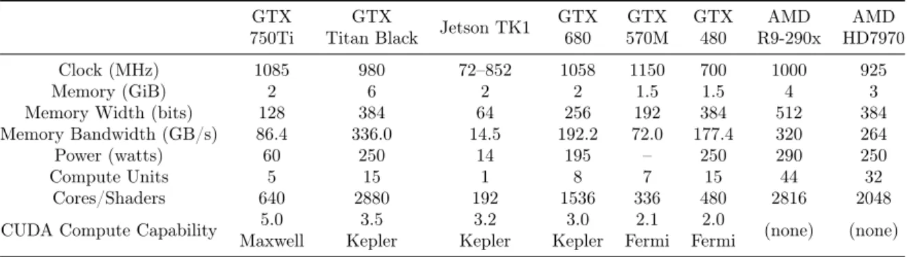
The Jetson CPU is classified by NVidia as a "4-PLUS-1" to reflect the ability of the system to enable/disable cores as needed for the interest of power conservation [19]. For this purpose, the CPU has 4 working cores and a low performance/low power usage core. This low performance core, identified as the "PLUS-1", drives the system when the computational demand is low. Whenever the computing load increases, the other cores are activated as needed. Conversely, when the load diminishes, the system scales back, shutting down cores as they are no longer required. Other features of the system to balance the computing power versus the power consumption are the ability to reduce/increase the memory operating frequency and to disable/enable support for I/O devices like USB and/or HDMI ports. In terms of hardware specifications, Jetson TK1 development board has a single CUDA multiprocessor (SMX), as further detailed in Table 2.2 alongside with the lists of available GPUs and their main characteristics. From the table, GPU GTX 570M refers to the laptop graphics card.
GTX 750Ti
GTX
Titan Black Jetson TK1 GTX 680 GTX 570M GTX 480 AMD R9-290x AMD HD7970 Clock (MHz) 1085 980 72–852 1058 1150 700 1000 925 Memory (GiB) 2 6 2 2 1.5 1.5 4 3 Memory Width (bits) 128 384 64 256 192 384 512 384 Memory Bandwidth (GB/s) 86.4 336.0 14.5 192.2 72.0 177.4 320 264 Power (watts) 60 250 14 195 – 250 290 250 Compute Units 5 15 1 8 7 15 44 32
Cores/Shaders 640 2880 192 1536 336 480 2816 2048 CUDA Compute Capability 5.0
Maxwell 3.5 Kepler 3.2 Kepler 3.0 Kepler 2.1 Fermi 2.0
Fermi (none) (none)
Table 2.2: GPU related Hardware Equipment Details.
The Raspberry is a low cost, low power, single board credit-sized computer, de-veloped by Raspberry Pi Foundation [17]. The Raspberry Pi has attracted a lot of attention, with both models of the first version – model A and model B. A major con-tributor for its popularity is the low price. Another contributing factor for the success of the Raspberry Pi is its ability to run a specially tailored version of Linux and the many applications it bears under the version 6 of the ARM architecture. The model B of version 2 of the Raspberry Pi, which is the one used in this study, was released in 2015. Model B – the high end model of the Raspberry Pi 2 – has a quad-core 32-bit ARM-Cortex A7 CPU operating at 900 MHz, a Broadcom VideoCore IV GPU and 1 GiB of RAM memory shared between the CPU and the GPU. Both the CPU and the GPU, and some control logic, are hosted in the Broadcom BCM 2836 SoC. The Raspberry Pi 2 maintains the low price base. Beside the doubling of the RAM memory, an important upgrade from the original Raspberry version lies in the CPU which has four cores and thus can be used for effective multithreading. Each CPU core has a 32 KiB instruction cache and a 32 KiB data cache, while a 512 KiB L2 cache is shared with all cores. Additionally, the fact that the CPU implements the version 7 of the
ARM architecture means that Linux distributions available for the ARM v7 can be run on the Raspberry Pi 2. The Raspberry Pi 2 maintains the same GPU of the original Raspberry Pi. The GPU is praised for its capability in decoding video, namely the ability to provide resolution of up to 1080 pixels (full HD) supporting the H.264 stan-dard [20]. However, to the best of our knowledge, no stanstan-dard parallel programming interfaces like OpenCL is available for the GPU of the Raspberry Pi. Another (minor) reported drawback is that the power consumption has increased from 3 watts for the Raspberry Pi 1 (model B) to 4 watts [21] in the Raspberry Pi 2 (model B).
As a final detail, for this dissertation, both Jetson and the Raspberry are referenced with distinguishable modes. By default, both Jetson and the Rasperry boot with their lowest (power saving) settings. We call these default "Jetson LowPower" and "Raspberry Def". After booting, both platforms/systems provide means to alter these settings. Only the high performance settings are used for comparison. Raspberry possesses a turbo mode that we identified as "Raspberry Turbo" which boosts the CPU from 700 MHz to 1000 Mhz and SDRAM from 400 MHz to 600 MHz, whereas the Jetson lets us tweak several of its components one by one. Because of this, we came up with 2 modes. One, "Jetson MaxFrequency", in which we only maximize the GPU related features, like boosting its clock rate from 72 MHz to 852 Mhz. And another, "Jetson MaxPerformance", where we simply set the maximum allowed values for all configurations plus: enable all four cores of the CPU; disable the CPU scaling by setting the scaling governator to performance mode; disable I/O devices (e.g., HDMI output); and inform the graphics card that no output is needed (by setting it to blank). None of these tweaks/boosts are overclock related, they are all within the hardware capabilities and no overheat was observed during this study.
2.2
Results Acquisition and Used Images
The next two chapters refer to two different algorithms that have different purposes. All execution time results shown in Chapter 3 are calculated through several execu-tions, i.e., they are the mean (x) of some amount of executions. Typically, execution time results related to Servers 1, 2 and 3 are calculated from the x of 30 executions. Execution times from the laptop system are calculated from 10 executions, while Jetson and Raspberry experiments used 5 and 3 execution, respectively. The lower number of execution/runs is to accommodate the huge execution times. Moreover, there is no need for very large mean calculations since all equipments provide results that are always within certain expected ranges. Tests were performed and all execution time results presented, on average, 0.8% standard deviation. Because these deviations are
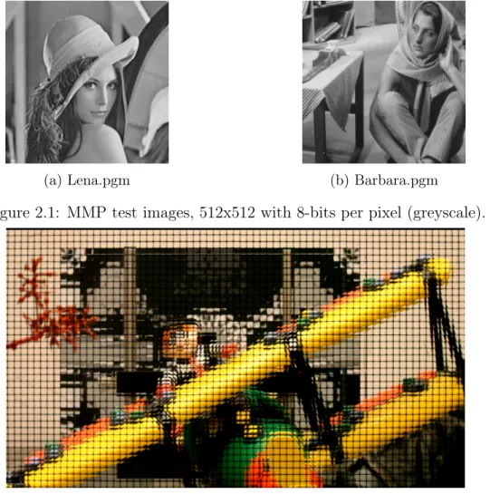
insignificant no other reference is made to them in this document. When larger de-viation were encountered the results were discarded and the test/benchmark redone. Also for Chapter 3, we used both Figures 2.1a and 2.1b as reference images. But since all the results had always the same properties — e.g. the second image achieved always faster results and always by the same proportions — and no image provided more interesting results over the other, results from Figure 2.1b were discarded thus not presented. Chapter 4 follows the same rules. Initially, we ran 5 executions per experiment, but due to the large execution time – several days per run – we scaled back to a simple execution per run. Here the standard deviations also do not have any meaningful weight. Of course, because the executions are so time consuming, small deviations may mean minutes, nevertheless, percentually, they never exceeded a 1.5% deviation. The experiment results in Chapter 4 were performed on the holoscopic image shown in Figure 2.2.
(a) Lena.pgm (b) Barbara.pgm
Figure 2.1: MMP test images, 512x512 with 8-bits per pixel (greyscale).
Figure 2.2: HEVC test image, frame 1 of 3D holoscopic test sequence Plane and Toy, size 1920x1088, captured using a 250µm pitch micro-lens array.
For the acquisition of sequential or non-GPU-driven implementation results, no discrete GPU cards were present in the underlying system, except the laptop, the Jetson and Raspberry equipments whose GPU is non-removable.
2.2.1
SpeedUp
As a way to simplify the comparisons made between results of different equipments and/or implementations the SpeedUp metric was applied. The SpeedUp metric shows the performance gain over a predetermined task between two systems processing the same problem or within the same system, but with different approaches to problem. Here the SpeedUp is calculated through:
SpeedUp = Base version time
New version time (2.1)
A speedup of 1 means that the two versions perform the computations in the same amount of time. A speedup in the range ]0; 1[ means that the new version suffered per-formance degradation. Finally, if the speedup is above 1 the new version is better/faster than the base version.
2.2.2
PSNR and Bitrate
Maintaining the program output when optimizing an algorithm is of utmost impor-tance. In image compression algorithms/software the output image is generally ac-companied by a value that tries to describe the quality loss that the image may have suffered. Peak signal-to-noise ratio, abbreviated PSNR, is an engineering term for the ratio between the maximum possible power of a signal and the power of corrupting noise that affects the fidelity of its representation. Because many signals have a very wide dynamic range, PSNR is usually expressed in terms of the logarithmic decibel scale. Basically, PSNR is an approximation to human perception of reconstruction quality – hence a measure of quality. Typical values for the PSNR in lossy image and video compression are between 30 and 50 dB, provided the bit depth is 8 bits, where higher is better. For 16-bit data typical values for the PSNR are between 60 and 80 dB – [22, 23]. PSNR is most easily defined via the mean squared error function. In statis-tics, the mean squared error (MSE) or mean squared deviation (MSD) of an estimator measures the average of the squares of the errors or deviations, that is, the difference between the estimator and what is estimated. In the absence of noise, two images are identical if the MSE is zero. In this case the PSNR is infinite.
Bitrate is the number of bits that are conveyed or processed per unit of time. The bit rate is quantified using the bits per second unit (symbol: “bit/s”). The non-standard
abbreviation “bps” is often alternatively used – like in the HEVC case.
2.3
Energy Measurements Methodology
Some of the results presented in this dissertation are related with energy consumption measurements. All energy consumptions were recorded with a MCP39F501 Power Monitor Demonstration Board [24] from Microchip. The board is a fully functional single-phase power monitor that does not use any transformers. The MCP39F501 Power Monitor Utility software is used to calibrate and monitor the system, and can be used to create custom calibration setups. The device calculates active power, reactive power, RMS current, RMS voltage, power factor, line frequency and other typical power quantities as defined in the MCP39F501 data sheet [25]. For any technical information, we refer the interested readers to [26].
The record of any of the executions starts with the direct connection of the MCP39F501 board to the laboratory wall outlet and to an USB port of the recording computer. From time to time (months), it is necessary to adjust the board software to correctly provide results over the input current so that accurate values are obtained. As soon as the board is powered and connected to the recording computer the recording loop is started. The recording computer queries the MCP39F501 board at 20 second intervals. The returned values include: current (Amps); voltage (Volts); active power (Watts); reactive power; apparent power; power factor; frequency (Hz); board sensor temper-ature (bits); and event flags. All the information is stored in a CSV format — plain text tabular data, including the date and time details. For this dissertation, we only considered the active power information. After starting the recording loop, the test equipment is connected to the output end of the MCP39F501 board, booted, and the target algorithm execution is started. In all tests, the equipments were linked to the same keyboard and monitor (with the exception of Jetson in MaxPerformance mode, which lacked the monitor output).
Because large numbers of records were expected, a separate log file was maintained with some relevant events (along side the date/time details). These include the clock time at which a given execution started or when the equipment being tested ended it OS boot.
After the target execution ends, the resulting data files were manually parsed to provide meaningful information. These include average watts consumed in the different
recording stages (connection, boot, OS login and preparation, algorithm execution, etc.). Between executions it was always included the bash “sleep 20s” command to allow the system to return to a stable power consumption and to separate the results in the CSV file.
For more accurate results, tests were performed to assess whether it would be better to execute several times a given target algorithm and work with the mean recorded power of several executions instead of just one. We concluded that it did not provide any improvement, besides a better estimate of the overall energy consumption a given algorithm may require for a given system. Therefore, presented energy results in this dissertation refer to a single execution.
2.4
Base Bandwidth Speeds
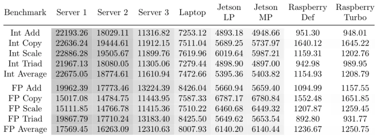
In order to quickly understand how our different hardware performs, we initially run several Phoronix benchmarks. The Phoronix Test Suite [27] is a testing and bench-marking platform available for several systems. We targeted the equipments RAM and CPU speeds in both bandwidth and instruction throughput. Table 2.3 provides a first performance comparison between the hardware/systems previously detailed in Table 2.1. Perceivable by the table greyscaled gradient, it is shown that Server 1 provides the best performance throughout several CPU operations and RAM memory accesses. The slightly different RAM architecture between Server 2 and Server 3 – 4x8GiB RAM per CPU for Server 2 vs 2x16GiB for Server 3 – becomes relevant here. In this benchmark, Server 3 has only mostly 3/5 of Server 2 capabilities, while the laptop only achieves 2/5 of Server 2 performance. As expected, SoC systems – Jetson and Raspeberry – have even worse performance with 3/10 and 2/25, respectively.
To complement the memory bandwidth measurements we also included the widely used Lempel-Ziv-Markov (LZMA) chain compression algorithm. The first idea of LZMA implementation was found in [28]. It was first used in the 7z format of the 7-Zip archiver [29]. This compression algorithm has proved to be effective in any byte stream compression for reliable lossless data compression. In order to benchmark our systems we resorted to the p7zip 9.20.1 tool [30] which already provides the bench-marking runtime. The LZMA benchmark shows a rating in MIPS (million instructions per second). The compression speed strongly depends on memory (RAM) latency and Data Cache size/speed. While the decompression speed strongly depends on CPU in-teger operations. The most important performance factors for the test are: branch
Benchmark Server 1 Server 2 Server 3 Laptop Jetson LP Jetson MP Raspberry Def Raspberry Turbo Int Add 22193.26 18029.11 11316.82 7253.12 4893.18 4948.66 951.30 948.01 Int Copy 22636.24 19444.61 11912.15 7511.04 5689.25 5737.97 1640.12 1645.22 Int Scale 22886.28 19505.67 11899.76 7619.96 6019.64 5987.21 1159.31 1202.76 Int Triad 21967.13 18080.05 11305.06 7279.44 4898.90 4897.00 942.98 989.95 Int Average 22675.05 18774.61 11610.94 7472.66 5395.36 5403.82 1154.93 1208.79 FP Add 19962.39 17773.46 13224.39 8426.04 5660.94 5659.40 1094.99 1157.55 FP Copy 15017.08 14784.75 11443.95 7587.33 6787.17 6780.84 1552.48 1651.85 FP Scale 15111.85 14766.78 11415.36 7510.22 6460.68 6449.32 1207.87 1259.45 FP Triad 19867.79 17710.24 13183.40 8425.50 5649.62 5653.54 892.80 931.77 FP Average 17569.45 16263.09 12310.63 8007.93 6140.20 6140.44 1236.67 1250.75
Table 2.3: RamSpeed Test Results for Integer and Floating Point operations from the Phoronix Test Suite 5.8.1 in MiB/s (more is better).
misprediction penalty (the length of pipeline) and the latencies of 32-bit instructions. The decompression test has very high number of unpredictable branches. Hence, the LZMA benchmark can accurately categorize our different systems.
Table 2.4 shows the resulting MIPS values for each system over the compression 2.4a and 2.4b algorithms. Analysis of the results yields similar conclusions to the one found for the Phoronix Test Suite (Table 2.3). To assess the systems we run the p7zip benchmark with a varying number of threads. With this information we can review how each CPU core behaves initially – with 1 thread – and how adding threads affects the results – in terms of MIPS. For the decompression algorithm, both Server 1 and SoC devices seem to take a performance hit.
Additionally, to provide some understanding over the laptop system – that can sometimes be more efficient than other hardware – we further reviewed its memory scheme. The Parallel Memory Bandwidth Benchmark (PMBW) [31] is a suite that measures bandwidth capabilities of a multi-core computer. This is an important test because more cores result in the floating point performance increasing in a linear fash-ion. However, if the memory bandwidth is not capable of transmitting the data fast enough, processors will stall. Indeed, unlike floating point units, memory bandwidth does not scale with the number of cores running in parallel. The PMBW code was developed in directly assembler language meaning inherent compiler issues such as op-timization flags will not occur. The code uses two general synthetic access patterns: sequential scanning and pure random access. The benchmark outputs an enormous amount of data, thus most of it was filtered out [32]. PMBW is already an accepted tool that provides large insight over the expected hardware performance [33, 34].
7zip
Threads Server 1 Server 2 Server 3 Laptop
Jetson Low Power Jetson Performance Raspberry Default 1 3460 3433 3379 3737 1602 1611 270 4 10026 9644 9515 8901 4565 4579 744 6 13992 13966 13333 11501 5099 5145 883 12 24086 23713 22826 15706 5146 5157 997 24 38090 37631 33939 15513 5142 5139 985 48 45646 42255 36805 15770 5085 5094 949
(a) LZMA Compressing Rating (MIPS)
7zip
Threads Server 1 Server 2 Server 3 Laptop
Jetson Low Power Jetson Performance Raspberry Default 1 2928 2797 2795 3206 2013 2030 401 4 11100 9916 9070 9849 7799 7926 1590 6 15561 13932 13427 12327 7282 7522 1553 12 26152 23510 23247 14614 7800 7814 1581 24 43734 39006 40761 14624 7761 7754 1578 48 42962 40337 40840 14518 7717 7723 1560
(b) LZMA Decompressing Rating (MIPS)
Table 2.4: LZMA compressing and decompressing benchmark results from the p7zip 9.20.1 in MIPS (more is better) with default dictionary size. The best result for each system is marked in bold.
laptop system and Server 1. The table is divided between Access Time and Bandwidth results, in nanoseconds and Gib per second, respectively. In terms of bandwidth, the laptop system presents a clear performance advantage in most of the scenarios, while keeping up in the remaining ones – these scenarios can be reviewed in at [31]. For a single thread the access time results confirm that the laptop provides data faster on average. The laptop has also higher reading performance, while Server 1 has higher storing/writing performance. But these results focus only over the utilization of 1 thread. The addition of other working threads change the performances. Table 2.6 shows the results for executions with different amounts of threads in a scenario where the laptop previously had more performance over Server 1 (with only 1 thread). These results show that while the laptop achieves better performance with 1 thread, Server 1 performs faster when multiple threads are used. While the laptop halts with average speeds of 0.7, Server 1 hardware continues to decrease its memory latency down to 0.17ns with 9 threads. The complex mesh of hardware characteristics of each device makes it challenging to accurately rate an equipment over the wide variety of appliances it may be a part of. Because of this, the laptop system may sometimes provide better results, since it sometimes performs better than other systems, making factors like memory access time, block/data sizes, buffers access patterns, etc., very important performance factors.
Benchmark Access Time Bandwidth
Server 1 Laptop Server 1 Laptop
ScanWrite256PtrSimpleLoop 4.1268 5.5326 41.18 32.31 ScanWrite256PtrUnrollLoop 4.7866 5.5329 41.18 33.12 ScanWrite128PtrSimpleLoop 2.0342 2.7651 39.50 43.40 ScanWrite128PtrUnrollLoop 2.3999 2.7591 41.31 45.64 ScanWrite64PtrSimpleLoop 1.1481 1.3962 20.44 16.49 ScanWrite64PtrUnrollLoop 1.0492 1.3810 20.73 16.47 ScanWrite32PtrSimpleLoop 0.5516 0.6898 10.31 11.38 ScanWrite32PtrUnrollLoop 0.5609 0.6892 10.38 11.47 ScanRead256PtrSimpleLoop 2.9367 2.9475 75.18 82.98 ScanRead256PtrUnrollLoop 2.9072 2.8877 82.47 89.26 ScanRead128PtrSimpleLoop 1.8558 1.5183 39.47 43.61 ScanRead128PtrUnrollLoop 1.6991 1.5020 80.98 89.40 ScanRead64PtrSimpleLoop 0.8346 0.8075 20.46 21.49 ScanRead64PtrUnrollLoop 0.9308 0.7898 41.13 44.99 ScanRead32PtrSimpleLoop 0.6071 0.4478 10.25 11.29 ScanRead32PtrUnrollLoop 0.5821 0.4434 20.67 22.79 ScanWrite64IndexSimpleLoop 0.9577 1.5099 20.45 22.54 ScanWrite64IndexUnrollLoop 1.1143 1.3824 20.70 22.86 ScanRead64IndexSimpleLoop 0.8700 0.8064 20.46 22.57 ScanRead64IndexUnrollLoop 1.0046 0.8102 41.04 43.70 PermRead64SimpleLoop 95.3199 73.9657 5.19 5.70 PermRead64UnrollLoop 94.2605 80.0693 5.19 4.11
Table 2.5: Access Time (in ns) and Bandwidth Results (in Gib/s) for all Benchmark Modes filtered from PMBW 0.6.2 with 1 thread over Server 1 and the Laptop (more Bandwidth is better and less Access Time is better, highlighted with grey).
Threads Access Time
Server 1 Laptop 1 0.9308 0.7898 2 0.4090 0.6891 3 0.3375 0.6859 4 0.2623 0.6854 5 0.2295 0.6915 6 0.2411 0.6881 7 0.1915 0.6944 8 0.1823 0.6971 9 0.1737 0.7375 10 0.1911 0.6934
Table 2.6: Access Time Results for ScanRead64PtrUnrollLoop Benchmark Mode fil-tered from PMBW 0.6.2 with 1–10 threads over Server 1 and the Laptop in nanoseconds (less is better, highlighted with grey).
Chapter 3
MMP – CPU, Many-Core,
Multi-Thread
In this chapter we present a small review of the selected algorithm (Section 3.1) and existing implementations (Section 3.2). With these building blocks, we further propose and implement a CPU multi-thread/multi-CPU version resorting to OpenMP (Section 3.3) and migrate an existing GPU implementation to CPU for further comparison (Section 3.4).
OpenMP was selected for this project due to its maturity and relatively high level abstraction. Other strategies were also analysed (e.g. MPI, compared in detail in [35]) but discarded since OpenMP has a lower learning curve [36, 37, 38] and is highly suited for multiprocessors multicore CPUs. A more low level approach, namely with POSIX Threads (PThreads), was also considered. However, it soon became apparent that many person-hours would be needed to achieve meaningful performance. Additionally, OpenMP proved to be suited for generating correct and structural parallel code as well as being capable of facilitating fine-grain improvements [39]. POSIX Threads implementations were therefore cast aside.
The migrated GPU implementation is based in the OpenCL API. Because OpenCL provides a vendor-neutral environment, i.e. enables implementations to be run in a large variety of components, OpenCL can thus be regarded as a "write once, run anywhere" (WORA) framework. However this does not implicitly mean that a source code which is optimal in a GPU environment will also deliver optimal performance for other components, namely CPUs. In this work, we demise the process of converting a GPU OpenCL optimized code for CPUs.
3.1
Multidimensional Multiscale Parser
The Multidimensional Multiscale Parser (MMP) is a pattern-matching-based compres-sion algorithm. Although it can compress any type of content [40, 41, 42], it is more appropriate for multimedia images [43, 44], where it lossy compression mode can achieve good compression ratio and maintain good image quality [1]. While compressing, MMP dynamically builds a dictionary of patterns that it uses for approximating the content of the input image [44]. Specifically, the input content is split in blocks, each having 16x16 pixels, and each input block is processed sequentially. For every input block, MMP assesses the patterns that exist in its dictionary in order to find the one that is the closest to the original one [44], that is, the one that yields the lowest overall dis-tortion. For this purpose, MMP needs to compute the Lagrangian cost J between the input block and all blocks existing in the dictionary. The Lagrangian cost is given by the equation J = D + λ ∗ R [45], where D measures the distortion between the original block and the candidate block, R represents the number of bits needed to encode the approximation and λ is a numerical configuration parameter, which remains constant along the execution of MMP. The λ parameter steers the algorithm towards more com-pression quality (low λ, which emphasizes the importance of low distortion over bit rate) or lower bit rate (high λ). MMP also explores patterns that are not yet in the dictionary, computing their Lagrangian cost J. This is done with the goal of finding new patterns that might be more suited for the input being processed, i.e., yield lowest Lagrangian cost. For these possible patterns to be, MMP uses a multiscale approach, which enables the approximation of image blocks with different sizes. Specifically, while the input image is processed in basic blocks of 16x16 pixels, all possible subscale blocks (8x4, 16x2, 1x1, etc.) are tested to find the best possible matches. When the search is exhausted, MMP selects the best block or set of sub-blocks, that is, the one(s) that delivers the lowest overall Lagrangian cost J. This exhaustive search is the main cause for the high computational complexity of MMP.
Having found a set of new blocks/sub-blocks, MMP proceeds to update the dictio-nary of patterns. However, first it checks whether the newly generated patterns already exist in the dictionary. To this extent, MMP lookups through the dictionary searching for blocks that might be identical or approximate (within a given radius) to the newly proposed blocks. If no close block to the new ones are found, MMP adds the new blocks/sub-blocks to the dictionary. The computing processes – block and sub-blocks search and dictionary update – is repeated for every single block of the input image. To facilitated dictionary searches, the dictionary is composed of sub dictionaries, each one for a subscale block size.
3.2
Previous Versions
Previously to this work, they were already three existing implementations of MMP: a sequential (CPU-driven) and two GPU-diven implementations. Although implemented with different languages/APIs, the two GPU versions are very similar, only differing on their API calls, i.e., their MMP logics are the same.
The denoted sequential implementation refer to the direct implementation of the MMP logic/algorithm with one CPU thread. The MMP algorithm is composed of sev-eral subparts/stages. The relevant stages for this dissertation are: (i) the initialization, (ii)the distortion calculation and tree segmentation, (iii) the dictionary actualization and (iv) the intra prediction modes. All these stages are presented in detail in [3, 44].
The (i) initialization and (iv) prediction modes parts become relevant in the later Section 3.3 and the (ii) distortion calculation and (iii) dictionary update for the GPU-driven implementations above and in Section 3.4.
The next subsections review the GPU-driven implementation (subsection 3.2.1) and present initial performance results obtained by the three existing implementations (subsection 3.2.2).
3.2.1
MMP-CUDA and MMP-OpenCL-GPU
The OpenCL and CUDA based versions [3, 2] are already optimized for GPUs. They consist on the migration of the sequential MMP algorithm in such way that it becomes possible to partially process all the sub blocks of a given larger block at once and later reduce the calculations in the same way that the original algorithm would had done it. The OpenCL-GPU implementation is a migration from CUDA whose conversion is described in [3]. Both versions use 4 kernels. Two major kernels to calculate the Lagrangian cost for each element of the dictionary of each subscale block size of the major block being processed (by the kernel named optimize_block) and to reduce the calculated values by selecting the less costing element of each subscale (by the kernel named j_reducter). After this process (in each image block), the natural order of things is to compare the findings and update the dictionary but since the GPU (CUDA/OpenCL targeted device) is doing part of the math around the dictionary, there is also the need to maintain its awareness on new selected findings between each
processed image block. As a solution, two minor kernels review the previous selected findings by comparing them to the existing ones on the dictionary (with the kernel compare_blocks) to determine if they are to be copied to the dictionary as new needed elements (with the kernel update_dic, so that the new dictionary is not copied as a whole from the host CPU after he also incorporates the new need elements). This last kernel is the one to actually update the device internal/mirror dictionary.
As in any optimized GPU implementation, important details must be taken care of in order to adieve the highest performance from the underlying hardware. In these implementations, the authors [3, 2] had the need to correctly balance the work between the different GPU workers/threads so that no group of workers ran out of work (since the dictionary is actually divided in several different sized subscale dictionaries). Not correctly balancing the work leads to branch diversion [46] which is a cause of execution delays. This is due to the fact that in-warp threads only re-converge after all divergent execution paths are completed [47]). Through the process of balancing the workload it is often necessary to flatten the access pattern to the memory data [48, 49]. This was also the case for MMP. Given the overall behaviour of the algorithm access patterns, in order to maintain the data locality [50], the dictionary data was laid out in such way that each individual worker did not need to access separated memory regions to obtain all data needed, nor it would generate misaligned access patterns within its group/warp. The goal is to provide a proper coalesced memory access, managing the issues data stride relate to. All of this simplifies other memory related optimizations, like the use of sequential addressing [51] for results reduction. As a last detail, the optimize_block kernel had the need for different local memory sizes between executions which let to less appropriate occupancy levels. To overcome this obstacle, since this particular local buffer directly depended on the number of possible prediction modes available for the given major block being processed, the kernel code was replicated 10 times, in which only the line declaring the local buffer size differed, ranging from numberOf KernelT hreads to numberOfKernelT hreads ∗ 10.
More detail about the CUDA and OpenCL implementations can be found in [3] and [2].
3.2.2
Base Reference Results
As a reference to the rest of this chapter, Tables 3.1 to 3.3 show the execution times registered for the pre-existing implementations on several hardware systems. For sim-plicity, the results are focused and compared (through speedup) with Server 2. Table 3.1 indicates the executions times encountered for the sequential implementation. The fastest execution times are recorded with the laptop system, followed by the servers. Jetson and Raspberry are without any doubt slower, yielding 2× and 12× times less performance, respectively. Regarding the CUDA implementation (Table 3.2), laptop 570M is still the fastest performer, unlike Jetson that only overtakes the sequential version when exiting Low Power mode. At its maximum performance, Jetson still only achieves around half the performance of the other systems. Table 3.3 shows the OpenCL-GPU results for NVidia and AMD GPUs. It is easily noticeable that NVidia, even when not using its primary language (CUDA), still performs better than AMD. From CUDA to OpenCL-GPU the execution time performance is degraded by around 40%. Time SpeedUp Server 1 2097.0340 1.03 Server 2 2157.7957 1.00 Server 3 2139.1510 1.01 Laptop 1836.5860 1.17 Jetson LP 5622.4783 0.38 Jetson MP 5558.7413 0.39 Raspberry Def 25734.4300 0.08 Raspberry Turbo 25415.6100 0.08
Table 3.1: Execution time results (in seconds) for the MMP-Sequential encoder for the Lena image with λ = 10 and dictionary size of 1024.
Time SpeedUp Sequential 2157.7957 1.00 GTX Titan 293.4368 7.35 GTX 680 299.5714 7.20 GTX 750Ti 298.7366 7.22 GTX 570M 287.5720 7.50 GTX 480 294.1414 7.34 Jetson LP 2638.3474 0.82 Jetson MF 1017.8993 2.12 Jetson MP 646.4966 3.34
Table 3.2: Execution time results (in seconds) for the MMP CUDA encoder for the Lena image with λ = 10 and dictionary size of 1024 for server 2.
Time SpeedUp Sequential 2157.796 1.00 GTX Titan 512.511 4.21 GTX 680 504.957 4.27 R9-290X 991.304 2.18 HD 7970 918.561 2.35
Table 3.3: Execution time results (in seconds) for the MMP OpenCL-GPU encoder for the Lena image with λ = 10 and dictionary size of 1024 for the servers 1 and 2 with NVidia and AMD GPUs — values from [3].
3.3
OpenMP
Open Multi-Processing is an Application Programming Interface (API) with a fork-join model. At its core level, OpenMP is a set of directives and callable library routines that are used to specify parallel computation in a shared memory style for C, C++, and Fortran [37, 52, 53] that influence run-time behaviour with the addition of envi-ronment variables [37]. The API is currently widely implemented by various vendors and open source communities [54]. OpenMP programming model can be used in a non-fragmented manner in contrast to other communication libraries and PGAS (Par-titioned Global Address Space) languages [55].
Figure 3.1: An illustration of the fork-join paradigm, in which three regions of the program permit parallel execution of the variously colored blocks. Sequential execution is displayed on the top, while its equivalent fork-join execution is at the bottom. — adapted from [56]
OpenMP is typically used after locating instances of potential parallelism within a sequential program. The section of code that is meant to run in parallel is marked with preprocessor directives. After the identification of loops in which parallel computation should occur, the OpenMP compiler and runtime implement its parallelism using a set of cooperating threads. By default, each thread executes a given parallelized section of code independently. The fork-join execution model (Figure 3.1) makes it easy to get loop-level parallelism out of a sequential program [52], with or without recursive forks, until a certain task granularity is reached. Recursively nested fork-joins can result in a parallel version of the divide and conquer paradigm [57, 58] (with e.g. quicksort [59]) that can reduce the overhead of task creation [60].
In contrast, querying the identity of a thread within a parallel region and taking actions based on that identity is also possible. This enables OpenMP to also be used in a fragmented manner, although it is more often used in a global-view manner, thus letting the compiler and runtime manage the thread-level details [53].
The idea behind OpenMP is to provide a predominantly open method of converting a sequential program into a multi-core, several-processor, application without any ma-jor code changes to the original source. All that is needed is to insert a few directives (or pragmas) into the pre-existing source code and enable the OpenMP compiler option [54] (e.g., "-fopenmp" in the GCC compiler). This triggers the compiler into checking for OpenMP directives and use the information they possess to transform the program for multithread execution, making the OpenMP implementation job to implicitly cre-ate the code necessary to run on different cores and/or processors. If OpenMP support is not ensured at compilation time, then the directives are ignored and the original single-threaded sequential code is generated. Only sections of code embraced by the directives are potentially translated. This is, if a few rules are observed, e.g. no data dependency between loop iterations. The rest of the program left untouched.
The ability to inject parallelism incrementally into a sequential program by the sim-ple addition of directives is considered the OpenMP greatest strength and productivity gain in addition to being a portable alternative to message passing.
With no explicit configuration, OpenMP generates a maximum number of threads equal to the number of present CPU cores (including hyper-threading [61, 62]). Obvi-ously, limitations to the number of threads generated also include code parallelization limits (e.g. a for-loop with a maximum of 5 cycles will only have 5 threads) and environment context, e.g., if some CPU cores are currently too busy with other com-putations, there is no point on adding more threads into their schedule. OpenMP
language extensions are divided in 5 constructs: thread creation, workload distribution (or sharing), data-environment management, thread synchronization, and user-level runtime routines and environment variables. Useful OpenMP technical and developer driven information can be found in [53].
To summarize and conclude, OpenMP was designed to enable the creation of, or transformation to, programs that are able to exploit the features of parallel computers where memory is shared. It enables the construct of portable parallel programs by supporting the developer at a high level with an approach that allows the incremental insertion of its constructs. Additionally, it also allows a conceivable low-level program-ming style, where the programmer explicitly assigns work to individual threads.
3.3.1
Profiling MMP-Sequential
Prior to the adaptation of MMP to multithread, the sequential version of MMP was profiled. Besides the opportunity to better understanding the original code mechanics and flow, profiling provides a means to rapidly spot more critically demanding sections. These sections are generally the most rewording candidates to be rearranged in a paral-lel fashion simply because they frequently point towards the code that is the more time consuming, making simple optimizations more noticeable [63]. Some experimentation was done with so called ‘Automatic Parallelization Tools’. However, none of the tested tools (ROSE1, PLuTo2 [64], CETUS3, iPat/OMP4 [65]) provided functional code, nor
any speedup.
The analysis of a sequential program performance often relies on profilers that provide statistical information about how much time is spent in different regions of code [66, 67]. Most active, or hot, regions are then given special attention. Tools like the open source [68] or the commercial Intel VTune [69] analyze programs at the function level. This may or may not directly include the creation of call-graph profiles that show the structure of the application at the functional level, including parent-child relationships and time spent in each function. To this extent, performance analysis tools intended to analyze sequential code are very mature. But this focus does not translate directly to tasks like extracting thread-level parallelism from applications. Although Intel VTune does lean in that direction since it is able to access Intel special
1ROSE: http://rosecompiler.org/
2PLuTo: http://pluto-compiler.sourceforge.net/
3CETUS: http://cetus.ecn.purdue.edu/
CPU registers/counters, it is a commercial product, thus out of the scope of this work.
A simplest way of profiling can be done by changing how every function in the program is compiled. This is done in such way that when they are called, it is possible to stash information about where the call came from. From here, is it possible to figure out what function called, count how many times a call happen, etc. This is actually one of the things achieved when the application is compiled with GCC with the "-pg" option does.
When trying to parallelize code, an intuitive first step might be to find which loops are doing most of the work. However, even deciding which loops to target (if any) can be very time consuming. Again, many free tools do not adequately capture the context, from a loop perspective, necessary to provide information about the consumed time. Some however, like LoopProf (introduced in [70]), depend on special instrumentations but then again do not leave guess work to the programmer like a call-graph profile leaves when trying to identify loops that are good candidates for parallelization. A somewhat extensive appreciation over several parallelization tools can be found in [71]. But since the ultimate goal is to use OpenMP, in the end, using this sort of tools does not provide much insight when balanced with the time spent reviewing different tools. Therefore, a more traditional/manual profiling was used for this work.
On a traditional side, it is common to see call-graph charts as a starting point for manual detection and determination of possible optimization-deficient sections. Like most applications, MMP spends a large portion of the execution time in small portions of code, typically inner loops. Tools such as GProf [72], OProfile [73], Intel VTune or DCPI [66] naturally identify such inner loops since they are the most frequently executed regions of code, but they do not focus on identifying loops themselves, thus failing to communicate information about the overall structure of loops in a program.
As stated and explained in [74], GProf quickly became, and still is, the tool of choice for many developers. Being based on the usage of the operating system interrupts, it is only necessary to compile the source code, in the case of GCC, with "-pg" option. Other considerations might also be important for a more loyal output when directly comparing with source code, e.g. not using inline function optimizations or even the "-O" options family (again, in GCC). When executing the application, the sampled data is saved (typically in a file named "gmon.out") just before the program exits. This is the data which is analysed by GProf. Several data files from different execution runs can be combined to a single file. Provided with this data and the source application, a textual, human readable, output is then generated.