Horizontal Injection of Gas–Liquid Mixtures in a Water Tank
Iran E. Lima Neto
1; David Z. Zhu, M.ASCE
2; and Nallamuthu Rajaratnam, F.ASCE
3Abstract:Experiments were carried out to investigate the behavior of horizontal gas–liquid injection in a water tank. Measurements of
bubble properties and mean liquid flow structure were obtained. The turbulence in the liquid phase appears to help generating bubbles with relatively uniform diameters of 1 – 4 mm. Both bubble properties and mean liquid flow structure depended on the gas volume fraction and the densimetric Froude number at the nozzle exit. It was found that the bubbles strongly affected the trajectory of the water jet, which behaved similarly to single-phase buoyant jets. However, at gas volume fractions smaller than about 0.15, the water jet completely separated from the bubble core. Bubble slip velocity was also found to be higher than the terminal velocity for isolated bubbles reported in the literature. Dimensionless correlations were proposed to describe bubble characteristics and the trajectory of the bubble plumes and water jets as a function of the gas volume fraction and the densimetric Froude number. Finally, applications of the results for aeration/ mixing purposes are presented.
DOI:10.1061/共ASCE兲0733-9429共2008兲134:12共1722兲
CE Database subject headings:Aeration; Bubbles; Jets; Mixing; Plumes; Gas; Water tanks; Froude number.
Introduction
Air and/or oxygen injection has long been used for artificial aera-tion and mixing in tanks, lakes, reservoirs, and rivers 共see, for example, Whipple and Yu 1970; WPCF 1988; Wüest et al. 1992; Schierholz et al. 2006; Bombardelli et al. 2007兲. Compared to the injection of single gas phase, the injection of gas–liquid mixtures has additional advantages, such as production of small bubbles without the need for porous diffusers, which are susceptible to clogging, and higher energy efficiency for aeration and mixing purposes共Amberg et al. 1969; Fast and Lorenzen 1976; Sun and Faeth 1986a,b; Iguchi et al. 1997; Mueller et al. 2002兲. Further, injection of oxygen into an effluent diffuser can also avoid the use of additional air diffusers in river aeration 共Lima Neto et al. 2007兲. In these types of flows, the oxygen transfer rate from the bubbles to the water is usually estimated using the following equation, derived from Fick’s law of diffusion共see Mueller et al. 2002兲:
dC
dt =KLa共Cs−C兲 共1兲
where C and Cs= dissolved oxygen 共DO兲 concentration in the water and the saturation concentration, respectively, KL= liquid
film coefficient or mass transfer coefficient; anda= air–water in-terfacial area per unit liquid volume or specific inin-terfacial area.
In water and wastewater systems such as aeration tanks, ponds, lagoons, and oxidation ditches, where the water depth is usually small compared to the water surface area, the use of hori-zontal gas–liquid injection is preferable rather than vertical gas– liquid injection in order to increase the contact time between the gas and liquid phases and, as a consequence, to increase the DO concentration in the liquid phase关see Eq.共1兲兴. In these systems, mixing chambers, Venturi tubes, or ejectors are generally used to mix the gas and the water and discharge the mixture as a series of two-phase buoyant jets that provide both aeration and mixing. These flows are a topic of growing interest because of their high oxygen transfer efficiency and low maintenance and operational costs 共Rainer et al. 1995; Morchain et al. 2000; Fonade et al. 2001; Mueller et al. 2002兲.
There are only limited experimental studies on horizontal gas– liquid injection. Varley共1995兲investigated the characteristics of the bubbles where bubble sizes were studied photographically and a correlation based on dimensional analysis for estimating the maximum bubble size was proposed. However, his study was limited to gas-volume fractions at the nozzle, , smaller than about 0.23, which is defined as
=Qa0/共Qa0+Qw0兲 共2兲
whereQa0andQw0= volumetric flow rates of air and water at the
nozzle, respectively. Besides, Varley’s measurements were taken only at the nozzle exit and at 10-15 nozzle diameters downstream of the nozzle exit, where bubble breakup and coalescence pro-cesses were assumed to be complete. Only bubble size measure-ments were provided with no other detailed information on bubble characteristics such as bubble velocity and specific inter-facial area. On the other hand, Morchain et al.共2000兲and Fonade et al.共2001兲ignored the buoyancy of the bubbles and estimated the flow circulation patterns induced by horizontal air–water in-jection in water assuming the same behavior of single-phase hori-zontal jets.
In this technical paper, we conduct an experimental study to
1
Ph.D. Candidate, Dept. of Civil and Environmental Engineering, Univ. of Alberta, Edmonton AB, Canada T6G 2W2. E-mail: limaneto@ ualberta.ca
2
Professor, Dept. of Civil and Environmental Engineering, Univ. of Alberta, Edmonton AB, Canada T6G 2W2. E-mail: david.zhu@ ualberta.ca
3
Professor Emeritus, Dept. of Civil and Environmental Engineer-ing, Univ. of Alberta, Edmonton AB, Canada T6G 2W2. E-mail: [email protected]
Note. Discussion open until May 1, 2009. Separate discussions must be submitted for individual papers. The manuscript for this paper was submitted for review and possible publication on August 22, 2007; ap-proved on June 7, 2008. This paper is part of theJournal of Hydraulic Engineering, Vol. 134, No. 12, December 1, 2008. ©ASCE, ISSN 0733-9429/2008/12-1722–1731/$25.00.
investigate bubble properties and mean liquid flow structure gen-erated due to horizontal air–water injection with gas volume frac-tions at the nozzle ranging from 0.13 to 0.63. The results obtained here are important for estimating the performance of jet aeration systems and to validate computational fluid dynamics 共CFD兲 codes for simulation of such flows.
Experimental Setup and Procedure
The tests were conducted in a rectangular glass tank with a length of 1.8 m, width of 1.2 m, and height of 0.80 m, shown schemati-cally in Fig. 1. The tank was filled with tap water to a depth of 0.76 m. The gas supply was taken from an air line, whereas the water was pumped from a small reservoir, and both air and water temperatures were fixed at about 20° C. A pressure-regulating valve was used to keep the air pressure at 1 atm 共gauge兲 and ensure a constant flow rate. Volumetric flow rates of air,Qa0, and
water, Qw0, were adjusted by rotameters; mixed into a Venturi
injector共Model 484, Mazzei Injector Corporation兲; and then dis-charged horizontally at the shorter plane of the tank through a single orifice nozzle of 0.6 cm in diameter, d0. The nozzle was
placed at the tank centerline with its exit located atx= 0 and z = 0共see Fig. 1兲. Table 1 summarizes the experimental conditions. Typical images of the bubbles for each experimental condition are shown in Fig. 2. A 500 W halogen lamp was used for back-ground illumination, and the images were acquired using a high resolution CCD camera共1,392⫻1,040 pixels兲共TM-1040, Pulnix Inc.兲controlled by a computer frame grabber system共Streams 5, IO Industries Inc.兲 with a frame rate of 30 frames per second 共fps兲and an exposure time of 1/2,000 s.
Measuring the turbulent liquid flow field within the bubble core using particle image velocimetry was difficult as our flows had relatively high void fractions. As a result, the laser light re-flected from the bubbles saturated the camera and corrupted the images of tracer particles. Alternatively, visualization of the en-trained liquid jet was achieved using laser-induced fluorescence 共LIF兲. A similar LIF system has been used by Socolofsky and Adams共2002兲for visualization of the entrained flow induced by bubble plumes.
Measurements of the mean vertical water velocity along the centerline of the bubble core and the water jet centerline outside the bubble core were performed at a height above the nozzle exit zof 24 cm with an electromagnetic propeller anemometer共Omni Instruments, MiniWater20兲 with an internal diameter of 22 mm 共see Fig. 1兲. This anemometer is suitable for velocities higher than 2 cm/s, with an accuracy of 2% when used in pure water. Similar propeller anemometers have been used to measure the mean ver-tical water velocity in bubble plumes and the measurement error due to air bubbles in the water is deemed negligible for local void fractions lower than 2.5% 共at z= 24 cm兲, as is the case in this study共see Milgram 1983; Riess and Fanneløp 1998兲. The reliabil-ity of our propeller anemometer for measuring vertical bubbly flows with void fractions of up to 3.5% was also confirmed by Lima Neto et al.共2008a兲. The measurements outside the bubble core were also verified with an acoustic Doppler velocimeter 共ADV兲 共SonTek 1997兲. This ADV can measure velocities from about 1.0 mm/s to 2.5 m/s at a sampling rate of 25 Hz.
A double-tip optical fiber probe system共RBI Instrumentation兲 based on the phase-detection technique was used to measure bubble properties. It consists of a module that emits infrared light through two fiber-optic cables to the tips of the probe, 2 mm apart. Each tip extends 1.5 cm and is sharpened into a 30m diameter. Emitted light is reflected back to the module when the tips pierce a bubble, resulting in a two-state signal which is re-corded at a sampling rate of up to 1 MHz. Absolute bubble ve-locity is obtained through a cross-correlation analysis of the signals from the two tips of the probe. The same system has been used to measure bubble properties in vertical bubble plumes and bubbly jets 共Lima Neto et al. 2008a,c兲 Similar RBI double-tip optical fiber probe systems have also been used for other bubbly flows共Boes and Hager 2003; Murzyn et al. 2005兲.
The optical probe signals were processed to calculate the local void fraction共␣兲, bubble frequency共fb兲, and absolute bubble ve-locity共ub兲and the following equations共see Chanson 2002兲were used to estimate the specific interfacial area 共a兲 and bubble volume-equivalent sphere diameter共db兲:
a= 4fb/u
b 共3兲
From water pump
180 cm
7
6
cm
Optical probe system
From air line Venturi
injector 32cm Bubble plume Water jet
L
W
x z
Anemometer and ADV
Bubbly jet
Surface jet
Fig. 1.Schematic of experimental setup
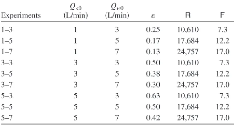
Table 1.Summary of Experimental Conditions: Gas Volume Fraction
共兲, Reynolds Number共R兲, and Densimetric Froude Number 共F兲Are Defined by Eqs.共2兲,共5兲, and共7兲, Respectively
Experiments
Qa0
共L/min兲
Qw0
共L/min兲 R F
1–3 1 3 0.25 10,610 7.3
1–5 1 5 0.17 17,684 12.2
1–7 1 7 0.13 24,757 17.0
3–3 3 3 0.50 10,610 7.3
3–5 3 5 0.38 17,684 12.2
3–7 3 7 0.30 24,757 17.0
5–3 5 3 0.63 10,610 7.3
5–5 5 5 0.50 17,684 12.2
5–7 5 7 0.42 24,757 17.0
db= 6␣/a 共4兲
The optical probe measurements were taken along the bubble core centerline at a height above the nozzle exitzof 24 cm, which was far enough for bubble breakup/coalescence processes to be complete and the bubbles to rise approximately in a rectilinear path.
A carriage mounted on the tank was used for both propeller anemometer and optical probe measurements in order to record data at different longitudinal distances from the nozzle, but the tests were conducted separately for each device. Each test was performed for a duration of 2 min共for each longitudinal distance from the nozzle兲, which was long enough to obtain stable mea-surements. The increase in water level due to water injection in the tank was less than 1% over the duration of each test, and this effect was considered negligible. This additional volume of water was then removed from the tank at the end of each test using an overflow pipe.
Experimental Results and Analysis
Bubble Properties
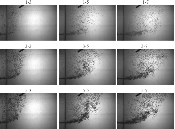
Typical images of the bubbles generated due to horizontal air– water injection in the tank are shown in Fig. 2. Relatively uniform bubbles with diameters ranging from about 1 to 4 mm were
observed visually. This is consistent with previous experimental results on vertical air–water bubbly jets共Lima Neto et al. 2008c兲, where bubbles with approximately uniform sizes were generated when the Reynolds number at the nozzle exit关given by Eq.共5兲兴 exceed a limit of aboutR= 8,000
R=Uw0d0/w 共5兲
where w= kinematic viscosity of water and Uw0= superficial
water velocity given by
Uw0=Qw0/共d0
2/4兲 共6兲
Approximately uniform bubble diameters, ranging from about 0.3 to 2 mm, were also observed photographically by Varley 共1995兲in his experiments on disperse horizontal bubbly jets with R⬎15,000, but the measurements were taken only at the nozzle exit and at 10–15 nozzle diameters downstream of the nozzle exit. Our preliminary tests withR⬍8,000 confirmed that for this con-dition the bubbles were much larger and irregular in size and shape, and the bubble core was much shorter. Therefore, the re-sults presented here are limited to experiments with R⬎8,000, which are expected to be more efficient for aeration purposes. All the following analyses in this technical paper will be based on the densimetric Froude number关given by Eq.共7兲兴, as both momen-tum and buoyancy forces are expected to affect the behavior of the air-water jets, similarly to single-phase buoyant jets共see Jirka 2004兲
1-3
1-5
1-7
3-3
3-5
3-7
5-3
5-5
5-7
Fig. 2.Typical images共32⫻50 cm2兲of the bubbles for each experimental condition, showing the tip of the optical probe located atx= 16 cm and
z= 24 cm
F=Uw0/
冑
g⬘d0 共7兲whereg⬘= reduced gravity given by
g⬘=g共w−a兲/
w 共8兲
in whichwanda= density of water and air, respectively. As sketched in Fig. 1, two regions are clearly observed in Fig. 2: a quasi-horizontal bubbly jet, where bubble breakup/ coalescence processes were observed visually; and a quasi-vertical bubble plume, where the bubbles rose approximately in a rectilinear path with no significant occurrence of breakup/ coalescence. Note that part of this bubble plume was formed by some coalesced bubbles that escaped from the quasi-horizontal bubbly jet, especially for the tests with higher values of and lower values ofF, where bubble coalescence processes appeared to dominate bubble breakup processes. Little lateral spreading of the bubble core from the horizontal bubbly jet to the quasi-vertical bubble plume was observed visually. Therefore, assuming that the width of the bubble core is equal to the average diameter of the quasi-horizontal bubbly jet 共W兲 and that the length of the bubble core is equal to the length of the bubble plume at z= 24 cm 共L兲 共see sketch in Fig. 1兲, we can see from Fig. 2 that the approximate width and length of the bubble core range from about 2 to 5 cm from and 17 to 40 cm, respectively, both increasing with the gas volume fraction and the densimetric Froude number. It can also be observed that the bubbly jet slightly deflects toward the vertical as the gas volume fraction increases.
A low-frequency lateral oscillation of the bubble core was also observed visually in the tests. The occurrence of such oscil-lations, also called wandering motions, is usually attributed to buoyancy driven instabilities and the effect of the tank walls共see Rensen and Roig 2001; García and García 2006; Lima Neto et al. 2008b兲. Fig. 3 shows typical void fraction and absolute bubble velocity time series measured with the optical fiber probe sys-tem. The average values of ␣ and ub are 1.2% and 0.6 m/s, respectively. The frequency of oscillation was about 0.05 Hz 共more clearly observed from the void fraction time series兲and the magnitude of the oscillations was smaller for the velocity time series.
Fig. 4 shows typical bubble size distributions fitted to mea-surements along the bubble plume centerline with a number of samples ranging from 70 to 900 bubbles for each experimental condition. For all experiments, the distribution resembles lognor-mal curves with average bubble diameters ranging from 1.8 to 3.4 mm and coinciding approximately with the peaks. Similar distributions were also obtained by Varley 共1995兲. The relatively narrow bands of the distributions confirm that the bubbles generated in our tests were approximately of uniform size, as mentioned earlier共see Fig. 2兲. It can also be seen that the
peaks increase along with the gas volume fraction with the result that more bubbles are generated共e.g., see curves for Experiments 1-3 and 5-3兲.
Fig. 5 shows the variations along the bubble core centerline of time-averaged void fraction共␣兲; bubble frequency共fb兲; absolute bubble velocity 共ub兲; bubble volume-equivalent sphere diameter
共db兲; and interfacial area共a兲, for each experiment. Figs. 5共a–c兲 show that ␣, f, anda follow approximately lognormal distribu-tions. It is clearly seen that the peaks increase as the gas volume fraction increases 共e.g., see Experiments 1-5, 3-5, and 5-5兲, whereas the bubble plumes become longer as the densimetric Froude number increases 共e.g., see Experiments 3-3, 3-5, and 3-7兲. The lengths of the bubble plumes obtained from Fig. 5 ranged from 18 to 44 cm, which are slightly higher than those obtained from the CCD images共see Fig. 2兲. Figs. 5共c and d兲show thatubanddbtend to increase as the flow approaches the location of the peak water velocity共see the following section兲. Note that for the experiments with lower densimetric Froude numbers共i.e., Experiments 1-3, 3-3, and 5-3兲, larger bubbles escaped from the weaker water jet and the bubble diameterdbseemed to decrease with the horizontal distance from the nozzle. Moreover, both ub anddbappear to increase with the gas volume fraction and de-crease with the densimetric Froude number. Similar results were obtained by Varley 共1995兲, who observed an increase indbwith the air flow rate and a decrease with the water flow rate. Bubble diameters shown in Fig. 5共d兲 ranged from 1.2 to 3.6 mm and were about 10% smaller than those obtained from the CCD cam-era images shown in Fig. 2, whereas bubble velocities shown in Fig. 5共c兲ranged from 41 to 77 cm/s and were about 25% larger
0.0 0.5 1.0 1.5 2.0 2.5 3.0
0 20 40 60 80 100 120
t (s)
α
(%
)
0.0 0.5 1.0 1.5 2.0 2.5 3.0
ub
(m
/s
)
Void fraction Bubble velocity
Fig. 3.Typical void fraction and absolute bubble velocity time series. Measurements taken atx= 28 cm andz= 24 cm共Experiment 3-5兲.
0 1 2 3 4 5 6 7 8 9
0 2 4 6 8 10 12
db(mm)
B
u
b
b
le
d
ia
m
e
te
r
p
o
p
u
la
ti
o
n
1-3 1-5 1-7
3-3 3-5 3-7
5-3 5-5 5-7
Fig. 4.Typical bubble size distributions obtained by fitting measure-ments taken atx= 16 cm andz= 24 cm
than those obtained from visual observation. Similar results were obtained with the same techniques in vertical bubble plumes and bubbly jets共Lima Neto et al. 2008a,c兲.
In order to make the results obtained here applicable to other horizontal gas–liquid injection conditions, dimensional analysis was conducted assuming that the forces due to viscosity, sur-face tension, and compressibility were negligible compared to the forces due to momentum and buoyancy, under fully turbu-lent flow conditions in a relatively shallow water tank. The horizontal gas–liquid jet is expected to be controlled by the kinematic fluxes of momentum 共controlled by the liquid phase兲 and buoyancy 共controlled by the gas phase兲, given by M0
=Qw0Uw0 and B0=Qa0g⬘, respectively. Thus the length and
velocity scales, Le andUe, can be defined as Le=M0 3/4/
B0 1/2 and
Ue=B0 1/2/
M0 1/4, or
Le=⌊共/4兲1 /4Fd
0⌋共Qw0/Qa0兲1
/2=⌊共/4兲1/4Fd
0⌋关共1 −兲/兴1 /2
共9兲
Ue=⌊共/4兲1 /4
冑
g⬘d0⌋共Qa0/Qw0兲1 /2
=⌊共/4兲1/4
冑
g⬘d0⌋关/共1 −兲兴1/2共10兲
Notice that the above-presented equations are extensions of those for single-phase buoyant jets. For example, for single-phase water jets where the buoyancy is created by temperature or salin-ity difference,B0=Qa0g⬘=Qw0g⬘, andQw0/Qa0in Eq.共9兲simply
becomes unity. In single-phase flows, Leis a useful length scale indicating where the buoyant jet changes from momentum
domi-nated to buoyancy domidomi-nated 共see Jirka 2004兲. In bubbly jet flows,Le is also expected to be a length scale where the bubbles separate from the water jet.
Using the above-presented scales, the following relationships can be obtained:
冋
LLe ,W
Le ,ub
Ue ,db
Le
,共KLa兲Le Ue
册
=f共,F兲 共11兲
Thus, measured values of the width共W兲and length共L兲of the bubble core as well as longitudinal-averaged values ofub,db, and KLa are nondimensionalized and curve fitting of experimental data provided the following correlations:
L Le
= 13.491共1.1F−0.1兲+ 0.168 共12兲
W Le
= 1.109共1.4F0.1兲+ 0.026 共13兲
ub Ue
= 1.598 ln共−1.2F−0.1兲+ 1.647 共14兲
db Le
= 2.103共1.1F−1.3兲+ 0.001 共15兲
0.0 0.5 1.0 1.5 2.0 2.5
0 10 20 30 40 50 60
x (cm) α (% ) 1_3 1_5 1_7 3_3 3_5 3_7 5_3 5_5 5_7 (a) 0.0 1.0 2.0 3.0 4.0 5.0 6.0 7.0 8.0
0 10 20 30 40 50 60
x (cm) f( H z ) 1_3 1_5 1_7 3_3 3_5 3_7 5_3 5_5 5_7 (b) 0.0 0.1 0.2 0.3 0.4 0.5 0.6 0.7 0.8 0.9
0 10 20 30 40 50 60
x (cm) ub (m /s ) 1_3 1_5 1_7 3_3 3_5 3_7 5_3 5_5 5_7 (c) 0 5 10 15 20 25 30 35 40 45
0 10 20 30 40 50 60
x (cm) a (m -1) 1_3 1_5 1_7 3_3 3_5 3_7 5_3 5_5 5_7 (e) 0.0 0.5 1.0 1.5 2.0 2.5 3.0 3.5 4.0
0 10 20 30 40 50 60
x (cm) db (m m ) 1_3 1_5 1_7 3_3 3_5 3_7 5_3 5_5 5_7 (d)
Fig. 5.Variations along the bubble core centerline of:共a兲void fraction;共b兲bubble frequency;共c兲absolute bubble velocity;共d兲bubble diameter; and共e兲specific interfacial area. Measurements shown were taken atz= 24 cm.
共KLa兲Le Ue
=关1.632⫻ln共−1.0F1.6兲− 4.977兴⫻10−3 共16兲
In the above-presented correlations, we used a constant mass transfer coefficient KL= 4⫻10−4m/s obtained for the range of bubble diameters studied here共see Wüest et al. 1992; McGinnis and Little 2002兲, which resulted in volumetric mass transfer co-efficients KLa ranging from about 7 to 37 h−1. Note that these correlations are valid for a specific height z= 24 cm above the nozzle exit.
Other length and velocity scales have also been used in dealing with gas–liquid two-phase flows. For example, Bombardelli et al.共2007兲defined a length scale D=B0/4␣e
2u s 3,
where ␣e= entrainment coefficient and us= bubble slip 共or
rela-tive兲 velocity. As both momentum and buoyancy at the nozzle are expected to be important in air–water jets, it is logical to define the length scaleLeand the velocity scaleUeas in Eqs.共9兲 and共10兲. These scales can be directly calculated from the flow conditions at the nozzle.
Fig. 6 shows that Eqs.共12兲–共16兲adjusted well to the experi-mental data, with coefficients of determination ranging from 0.971 to 0.997. This suggests that the parameters adopted here are appropriate to describe the dynamics of the bubbles generated from horizontal gas–liquid injection. Note that we also tested
dif-ferent length scales such as the above-mentionedDand a param-eter given byLe*=共Q2w0/g兲1/5, as well as different velocity scales defined asUD=Qw0/D2andUe*=Qw0/共Le*兲2, but the resulting
cor-relation equations did not adjust that well to the experimental data.
The length scaleLeis proportional tod0whereas the velocity
scale Ue is proportional to
冑
do for the same values of andF. Hence, if we had for instance a nozzle diameter 2.5 times larger and flow rates 10 times higher than those used in this study共 keep-ingandFconstant兲, we would expect bubbles with a diameter and velocity of, respectively, 2.5 and 1.6 times larger. Neverthe-less, caution should be taken when using Eqs.共12兲–共16兲for scal-ing up of jet aerator systems with much larger nozzle diameters, as the bubble diameter in similar flows 共i.e., vertical bubble plumes兲is expected to be up to about 40 mm关see the summary in Bombardelli et al.共2007兲兴.Liquid Flow Structure
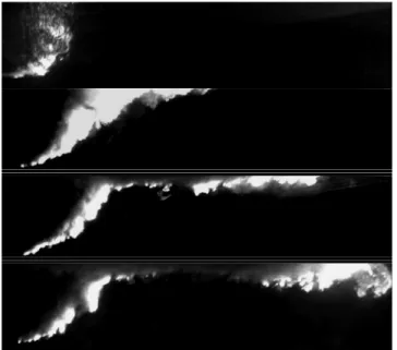
Fig. 7 shows a typical sequence of LIF images of the water jet. As sketched in Fig. 1, this water jet follows approximately the tra-jectory of the bubbles in the bubbly jet region 共as momentum dominates buoyancy forces兲, partially separates from the bubble 0
1 2 3 4 5 6 7 8
0.0 0.2 0.4 0.6
ε ε1.1Fr-0.1
L
/
Le
Experiments Eq. (12)
(a)
0 1 2 3 4 5 6
0 2 4 6 8 10
ε ε-1.2Fr-0.1
u
b
/
U
e
Experiments Eq. (14)
(c)
0.00 0.02 0.04 0.06 0.08 0.10 0.12
0.00 0.01 0.02 0.03 0.04 0.05
ε ε1.1Fr-1.3
d
b
/
L
e
Experiments Eq. (15)
(d)
0E+00 1E-03 2E-03 3E-03 4E-03 5E-03 6E-03 7E-03
0 200 400 600 800
ε ε-1.0Fr1.6
K
L
a
L
e
/
U
e
Experiments Eq. (16)
(e) 0.0
0.1 0.2 0.3 0.4 0.5 0.6 0.7 0.8 0.9 1.0
0.0 0.2 0.4 0.6 0.8
ε ε1.4Fr0.1
W
/
L
e
Experiments Eq. (13)
(b)
Fig. 6.Adjustment of the dimensionless correlations for共a兲length of the bubble core;共b兲width of the bubble core;共c兲absolute bubble velocity;
共d兲bubble diameter; and共e兲volumetric mass transfer coefficient to experimental data. The error bars indicate deviations of 10% from the mean values, which were estimated from sample tests of reproducibility of the results.
core after some distance from the nozzle共as the bubbles tend to move upwards due to buoyancy forces兲, and then becomes a sur-face water jet. This behavior is similar to that of single-phase buoyant jets described by Jirka共2004兲, except for the separation phenomenon, which has also been observed in bubble plumes in crossflows 共see Socolofsky and Adams 2002兲. The LIF images also showed that recirculation currents formed about 1 min after the beginning of the tests, and oscillations in their position during the experiments probably contributed to the above-mentioned wandering motion of the bubble core, as observed by Lima Neto et al.共2008b兲in vertical bubble plumes.
Calculating the horizontal water velocity at the surface jet re-gion from the LIF images, we can estimate the volumetric mass transfer coefficient due to surface aeration at the air–water inter-face using predictive equations given by Lima Neto et al.共2007兲. For example, considering a horizontal water velocity of about 5 cm/s共see Fig. 7兲and the water depth of 76 cm, we estimated a volumetric mass transfer coefficient of the order of 0.05 h−1
for Experiment 3-5, which is much smaller than the corre-spondingKLavalue of 22 h−1estimated earlier for mass transfer from the bubbles to the water. This implies that most of the oxy-gen transferred to the water is due to bubble dissolution, even though the contact area between the bubbles and the water is about 20 times smaller than that between the atmosphere and the water.
Part of the water jet inside the bubble core could not be visu-alized from LIF images because the bubbles blocked the laser sheet. However, propeller anemometer measurements of vertical water velocity, 共u兲, shown in Fig. 8, confirmed that significant velocities were present inside the bubble core, with the velocity distributions roughly resembling lognormal curves. This occurred because of additional entrainment into the wakes of the bubbles, as observed by Leitch and Baines 共1989兲 and Lima Neto et al. 共2008c兲in experiments with vertical bubble plumes and bubbly jets, respectively. Fig. 8 also shows that the magnitude of the
velocities and the penetration lengths increase along with the gas volume fraction共see Experiments 1-5, 3-5 and 5-5兲, whereas in-creases in the densimetric Froude number increase the penetration lengths but decrease the peak velocities 共see Experiments 3-3, 3-5, and 3-7兲. It is important to mention that a distinct behavior was observed for Experiment 1-7, where the water jet completely separated from the bubble core at aboutx= 40 cm and two peaks are present in the vertical water velocity profiles shown in Fig. 8: one at about x= 30 cm due to the flow induced by the bubble plume and another at aboutx= 65 cm due to the water jet itself. This separation was mainly attributed to the relatively small buoyancy as compared to the high momentum of the water jet 共see Table 1兲. We can thus conclude that a transition gas volume fraction lies between the values of 0.17 and 0.13, which corre-spond to Experiments 1-5 and 1-7, respectively. We propose that a value ofsmaller than about 0.15 is needed to cause complete separation between the bubble core and water jet.
Trajectory of the Bubble Plumes and Water Jets
Following the procedure described earlier to obtain Eq.共11兲, di-mensional analysis gives these relationships to describe, respec-tively, the trajectory of the bubble plumes and water jets
冉
zbLe
冊
=f
冉
,F,xb Le冊
共17兲
冉
zwLe
冊
=f
冉
,F,xw Le冊
共18兲
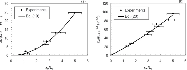
Hence, assuming that the center of the bubble plumes coin-cides with the location of the peak void fraction measurements 关see Fig. 5共a兲兴, we can normalize our data and obtain the follow-ing correlation to describe the trajectory of the bubble plumes:
zb Le=
−1.7F−1.0
冋
0.983冉
xb Le冊
2
− 0.069
冉
xbLe
冊
册
共19兲Fig. 9共a兲 shows that Eq.共19兲fits well to the experimental data, with a coefficient of determination of 0.987. Similarly, assuming that the center of the water jets coincides with the location of the peak vertical water velocities共see Experiment 3-5 in Figs. 7 and 8兲, we obtain the following correlation to describe the trajec-tory of the water jets:
Fig. 7. Typical sequence of LIF images 共32⫻140 cm2兲 at times
t= 0.0, 6.7, 13.3, and 20.0 s after dye injection 共Experiment 3-5兲. Note that the bubbles are shown in the first image and the water jet development is shown in the subsequent images. Part of the water jet inside the bubble core cannot be visualized because the bubbles blocked the laser sheet.
0.00 0.05 0.10 0.15 0.20 0.25 0.30
0 20 40 60 80 100 120
x (cm)
u
(m
/s
)
1-3 (Anem.) 1-5 (Anem.) 1-7 (Anem.) 3-3 (Anem.) 3-5 (Anem.) 3-5 (ADV) 3-7 (Anem.) 5-3 (Anem.) 5-5 (Anem.) 5-7 (Anem.)
Fig. 8.Typical variations of mean vertical water velocity along the bubble plume/water jet centerline. Measurements shown were taken atz= 24 cm.
zw Le
=−0.5F−1.4
冋
0.797冉
xw Le冊
2
+ 14.673
冉
xw Le冊
册
共20兲
Fig. 9共b兲 shows that Eq.共20兲 also fits well to the experimental data, with a coefficient of determination of 0.988. Note that experimental data corresponding to Experiment 1-7 共 ⬍0.15兲 was excluded from this figure because, in this case, the water jet separated completely from the bubble core, as mentioned ear-lier. Eq.共20兲 is important because models for simulation of the flow induced by jet aerator systems usually assume that the be-havior of the horizontal water jet is not affected by the bubbles 共see Morchain et al. 2000; Fonade et al. 2001兲.
Bubble Slip Velocity and Shape
With the measurements of vertical water velocity and absolute bubble velocity, we can now estimate the bubble slip velocity,us. Fig. 10 shows that bubble slip velocities obtained in this study ranged from about 0.3 to 0.5 m/s and collapsed well within the curve proposed by Lima Neto et al.共2008c兲to describe the varia-tion ofuswithdbin vertical bubbly flows. The above-mentioned values are higher than the terminal bubble velocity of about 0.2 m/s given by Clift et al.共1978兲for isolated bubbles of similar diameters. This occurred because trailing bubbles in the wake of leading bubbles rise faster than isolated bubbles due to drag re-duction, as observed by Ruzicka 共2000兲 on experiments on bubbles rising in line. The results shown in Fig. 10 are important because models for simulation of bubbly flows usually assume constant slip velocities equal to the terminal bubble velocities given by Clift et al.共1978兲.
Using the values ofusanddbestimated earlier, we can calcu-late the bubble Reynolds number共Rb=usdb/w兲, Eötvös number
共Eb=g⌬db
2/兲, and Morton number共M
b=g⌬w 4/
w
23兲, where
⌬= difference between the water and air densities;= air–water surface tension; andw= viscosity of water. These dimensionless numbers are generally used to express the importance of inertia, buoyancy, surface tension, and viscosity on single bubbles rising
in liquids. For the present study, the ranges of RbandEb were 480–1755 and 0.2–1.7, respectively, andMb= 3.1⫻10−11.
Accord-ing to the classical diagram describAccord-ing the behavior of isolated bubbles provided by Clift et al.共1978兲, our values ofRb,Eband Mb fall within the region of spherical, ellipsoidal, and wobbling regimes, which is in agreement with the shapes observed from the CCD images 共see Fig. 2兲. This trend suggests that the bubbles studied here behaved similarly to isolated bubbles, although their slip velocities were higher. Similar results were obtained by Lima Neto et al.共2008c兲for vertical bubbly jets.
Applications
The correlations obtained here can be used for the scaling up of jet aerator systems, as mentioned earlier, as well as to compare the aeration potential of different horizontal air–water injection
10 100 1000
1 10 100
db(mm)
u
s
(c
m
/s
)
Present study
Lima Neto et al. (2007)
Clift et al. (1978) (2008c)
Fig. 10. Bubble slip velocity versus bubble diameter. Dashed and solid lines indicate fitted curves obtained from the literature pertaining to isolated bubbles and vertical bubbly flows, respectively.
0 5 10 15 20 25 30
0 1 2 3 4 5 6
xb/Le zb
/(
Le
ε
-1
.7
F
r
-1
.0 )
Experiments
Eq. (19)
(a)
0 20 40 60 80 100 120
0 1 2 3 4 5 6
xw/Le
zw
/(
Le
ε
-0
.5
F
r
-1
.4 )
Experiments
Eq. (20)
(b)
Fig. 9. 共a兲 Dimensionless trajectory of the bubble plumes; 共b兲 dimensionless trajectory of the water jets. Note that data corresponding to Experiment 1-7 共with ⬍0.15兲 are excluded from the dimensionless trajectory of the water jets because of the occurrence of complete separation from the bubble plume. The error bars indicate deviations of 10% from the mean values, which were estimated from sample tests of reproducibility of the results.
conditions. Defining this aeration potential as the product of the volumetric mass transfer coefficient 共KLa兲 by the approximate area of the bubble core in contact with the water column above the nozzle 共W⫻L兲, we can estimate, for example, which flow condition studied here is the best for aeration. Fig. 11 shows that, as expected, the experiment with the highest air and water flow rates共Experiment 5-7兲corresponds to the best condition for aera-tion. On the other hand, experiments with relatively high air flow rates and low water flow rates共e.g., Experiment 5-3兲 may have comparable aeration potential to those with relatively low air flow rates and high water flow rates 共e.g., Experiment 3-5兲, which in turn will result in higher electricity costs for pumping a higher water flow rate. However, in this case, the benefit will be a higher penetration length of the water jet for circulation and mix-ing as compared to the experiments with lower water flow rates 共see Fig. 8兲. It is important to stress that all experiments con-ducted here were performed forR⬎8,000, where bubbles of ap-proximately uniform sizes were generated. For lower values ofR, we expect the formation of larger bubbles and reduced aeration potential, as mentioned earlier. Therefore, we recommend that the condition ofR⬍8,000 should be avoided.
Overall, the above-presented results of bubble properties and mean liquid flow structure can also be used to evaluate and vali-date CFD models for horizontal gas–liquid injection systems. However, caution should be taken when applying these results to systems with different temperatures and high concentration of im-purities, which could impact on the two-phase flow behavior and mass transfer characteristics共see Clift et al. 1978; Mueller et al. 2002兲.
Summary and Conclusions
An experimental study was performed to investigate the behavior of horizontal injection of air–water mixture in a water tank. The experimental conditions included gas volume fractions ranging from 0.13 to 0.63, Reynolds numbers ranging from 10,600 to 24,800, and densimetric Froude numbers ranging from 7 to 17, which produced bubbles of approximately uniform size with volume-equivalent sphere diameters ranging from about 1 to 4 mm.
Two important regions were observed from the images of the bubbles: a quasi-horizontal bubbly jet and a quasi-vertical bubble plume. Bubble size distributions obtained by fitting measurements at the bubble plume region resembled lognormal curves with rela-tively narrow bands. This confirmed that the bubbles generated in our tests were approximately of uniform size. Time-averaged dis-tributions of bubble properties along the bubble core centerline were found to depend on the gas volume fraction and the densi-metric Froude number. The distributions of void fraction, bubble
frequency, and interfacial area followed approximately lognormal distributions. On the other hand, absolute bubble velocity and bubble diameter tended to increase with the horizontal distance from the nozzle exit, except for the experiments with higher gas volume fractions and lower densimetric Froude numbers, where larger bubbles escaped from the weaker water jet closer to the nozzle exit. Dimensionless correlations for bubble properties and the trajectory of the bubble plumes as a function of the gas vol-ume fraction and the densimetric Froude number were also ob-tained by curve fitting of experimental data.
It was found that the water jet followed approximately the trajectory of the bubbles in the bubbly jet region, partially sepa-rated from the bubble core after some distance from the nozzle, and then became a surface water jet. Both the peak vertical water velocities and the trajectory of the water jets were found to de-pend on the gas volume fraction and the densimetric Froude num-ber. However, it was found that the water jet completely separated from the bubble core at gas volume fractions smaller than about 0.15. Excluding such particular conditions, a dimensionless cor-relation for the water jet trajectory as a function of the gas volume fraction and the densimetric Froude number was also obtained by curve fitting of experimental data. This correlation is important because current models for simulation of the flow generated by horizontal gas–liquid injection usually assume that the trajectory of the water jet is not affected by the presence of the bubbles.
In the above-mentioned correlations, the parameters were nor-malized by appropriate length and velocity scales defined as func-tions of the kinematic fluxes of momentum and buoyancy, similarly to those used for single-phase buoyant jets. Provided the gas volume fraction and densimetric Froude number follow the principle of similitude, these correlations are expected to be con-sistent for purposes of scaling up jet aerator systems. However, as the length scale used in these correlations is proportional to the nozzle diameter and we expect that there is a limit for the maxi-mum bubble size in field-scale bubble plumes, caution should be taken when scaling up jet aerator systems with much larger nozzle diameters.
Bubble slip velocities were found to be higher than the termi-nal velocities for isolated bubbles reported in the literature, even though their shapes were similar for the same values of Reynolds, Eötvös, and Morton numbers. This was attributed to the fact that trailing bubbles in the wake of leading bubbles rise faster than isolated bubbles due to drag reduction, as reported in the literature pertaining to bubbles rising in line. Bubble slip velocities ob-tained here could be described as a function of bubble diameter and adjusted well to the curve proposed by Lima Neto et al. 共2008c兲for vertical bubble plumes and bubbly jets. These results are important because two-phase models for vertical bubbly flows typically assume bubble slip velocities of the same order as those for isolated bubbles.
Finally, applications of the results for estimation of the aeration/mixing potential of different horizontal air–water injec-tion condiinjec-tions are presented and discussed.
Acknowledgments
The first writer is supported by the Coordination for the Improve-ment of Higher Education Personnel Foundation共CAPES兲, Min-istry of Education, Brazil. The writers would like to thank Perry Fedun and Chris Krath for building the experimental apparatus.
0.0 0.1 0.2 0.3 0.4 0.5 0.6
1-3 1-5 1-7 3-3 3-5 3-7 5-3 5-5 5-7
Experiments KL
a
x
W
x
L
(m
2/h
)
Fig. 11.Estimated aeration potential for each experimental condition
Notation
The following symbols are used in this paper: a ⫽ air–water specific interfacial area共m−1兲;
B0 ⫽ kinematic flux of buoyancy defined byB0=Qa0g⬘
共m4/s3兲;
C ⫽ dissolved oxygen共DO兲concentration in water 共mg/L兲;
Cs ⫽ saturation DO concentration in water共mg/L兲; db ⫽ bubble volume-equivalent sphere diameter共mm兲; d0 ⫽ nozzle diameter共cm兲;
F ⫽ densimetric Froude number defined by Eq.共7兲; f ⫽ bubble frequency共Hz兲;
g⬘ ⫽ reduced gravity defined by Eq.共8兲共m/s2兲;
KL ⫽ mass transfer coefficient共m/s兲;
L ⫽ length of the bubble core defined in Fig. 1共cm兲; Le ⫽ length scale defined byLe=M0
3/4/
B0
1/2or Eq.共9兲 共cm兲;
M0 ⫽ kinematic flux of momentum defined byM0=Qw0Uw0
共m4/s2兲;
Qa0 ⫽ air flow rate at the nozzle共L/min兲;
Qw0 ⫽ water flow rate at the nozzle共L/min兲;
R ⫽ Reynolds number defined by Eq.共5兲; Ue ⫽ velocity scale defined byUe=B0
1/2/
M0
1/4or Eq.共10兲
共cm/s兲;
Uw0 ⫽ superficial water velocity at the nozzle exit共cm/s兲;
u ⫽ vertical water velocity共m/s兲; ub ⫽ absolute bubble velocity共m/s兲; us ⫽ bubble slip velocity共m/s兲;
W ⫽ width of the bubble core defined in Fig. 1共cm兲; x ⫽ horizontal distance from the nozzle exit defined in
Fig. 1共cm兲;
xb ⫽ horizontal position of the bubble plume centerline 共cm兲;
xw ⫽ horizontal position of the water jet centerline共cm兲; z ⫽ vertical distance from the nozzle exit defined in
Fig. 1共cm兲;
zb ⫽ vertical position of the bubble plume centerline共cm兲; zw ⫽ vertical position of the water jet centerline共cm兲;
␣ ⫽ air concentration or local void fraction共%兲; and ⑀ ⫽ gas volume fraction at the nozzle defined by Eq.共2兲.
References
Amberg, H. R., Wise, D. W., and Aspitarte, T. R. 共1969兲. “Aeration of streams with air and molecular oxygen.” Tappi J., 52共10兲, 1866–1871.
Boes, R. M., and Hager, W. H.共2003兲. “Two-phase flow characteristics of stepped spillways.”J. Hydraul. Eng., 129共9兲, 661–670.
Bombardelli, F. A., Buscaglia, G. C., Rehmann, C. R., Rincón, L. E., and García, M. H. 共2007兲. “Modeling and scaling of aeration bubble plumes: A two-phase flow analysis.”J. Hydraul. Res., 45共5兲, 617–630.
Chanson, H.共2002兲. “Air-water flow measurements with intrusive, phase-detection probes: Can we improve their interpretation?”J. Hydraul. Eng., 128共3兲, 252–255.
Clift, R., Grace, J. R., and Weber, M. E. 共1978兲. Bubbles, drops and particles, Academic, New York.
Fast, A. W., and Lorenzen, M. W.共1976兲. “Synoptic survey of hypolim-netic aeration.”J. Envir. Engrg. Div., 102共6兲, 1161–1173.
Fonade, C., Doubrovine, N., Maranges, C., and Morchain, J. 共2001兲. “Influence of a transverse flowrate on the oxygen transfer perfor-mance in heterogeneous aeration: Case of hydro-ejectors.”Water Res.,
35共14兲, 3429–3435.
García, C. M., and García, M. H.共2006兲. “Characterization of flow tur-bulence in large-scale bubble-plume experiments.” Exp. Fluids,
41共1兲, 91–101.
Iguchi, M., Okita, K., Nakatani, T., and Kasai, N.共1997兲. “Structure of turbulent round bubbling jet generated by premixed gas and liquid injection.”Int. J. Multiphase Flow, 23共2兲, 249–262.
Jirka, G. H. 共2004兲. “Integral model for turbulent buoyant jets in un-bounded stratified flows. I: Single round jet.” Environmental Fluid Mechanics, 4共1兲, 1–56.
Leitch, A. M., and Baines, W. D.共1989兲. “Liquid volume flux in a weak bubble plume.”J. Fluid Mech., 205, 77–98.
Lima Neto, I. E., Zhu, D. Z., and Rajaratnam, N.共2008a兲. “Air injection in water with different nozzles.”J. Environ. Eng., 134共4兲, 283–294. Lima Neto, I. E., Zhu, D. Z., and Rajaratnam, N. 共2008b兲. “Effect of
tank size and geometry on the flow induced by circular bubble plumes and water jets.”J. Hydraul. Eng., 134共6兲, 833–842.
Lima Neto, I. E., Zhu, D. Z., and Rajaratnam, N.共2008c兲. “Bubbly jets in stagnant water.”Int. J. Multiphase Flow, in press.
Lima Neto, I. E., Zhu, D. Z., Rajaratnam, N., Yu, T., Spafford, M., and McEachern, P.共2007兲. “Dissolved oxygen downstream of an ef-fluent outfall in an ice-covered river: Natural and artificial aeration.” J. Environ. Eng., 133共11兲, 1051–1060.
McGinnis, D. F., and Little, J. C. 共2002兲. “Predicting diffused-bubble oxygen transfer rate using the discrete-bubble model.” Water Res.,
36共18兲, 4627–4635.
Milgram, H. 共1983兲. “Mean flow in round bubble plumes.” J. Fluid Mech., 133, 345–376.
Morchain, J., Moranges, C., and Fonade, C.共2000兲. “CFD modelling of a two-phase jet aerator under influence of a crossflow.” Water Res.,
34共13兲, 3460–3472.
Mueller, J. A., Boyle, W. C., and Pöpel, H. J.共2002兲.Aeration: Principles and practice, CRC, New York.
Murzyn, F., Mouaze, D., and Chaplin, J. R.共2005兲. “Optical fibre probe measurements of bubbly flow in hydraulic jumps.”Int. J. Multiphase Flow, 31共1兲, 141–154.
Rainer, B., Fonade, C., and Moser, A.共1995兲. “Hydrodynamics of a new type of ejector.”Bioprocess Eng., 13共2兲, 97–103.
Rensen, J., and Roig, V. 共2001兲. “Experimental study of the unsteady structure of a confined bubble plume.”Int. J. Multiphase Flow, 27共8兲, 1431–1449.
Riess, I. R., and Fanneløp, T. K.共1998兲. “Recirculation flow generated by line-source bubble plumes.”J. Environ. Eng., 124共9兲, 932–940. Ruzicka, M. C.共2000兲. “On bubbles rising in line.”Int. J. Multiphase
Flow, 26共7兲, 1141–1181.
Schierholz, E. L., Gulliver, J. S., Wilhelms, S. C., and Henneman, H. E.
共2006兲. “Gas transfer from air diffusers.”Water Res., 40共5兲, 1018– 1026.
Socolofsky, S. A., and Adams, E. E. 共2002兲. “Multi-phase plumes in uniform and stratified crossflow.”J. Hydraul. Res., 40共6兲, 661–672. SonTek.共1997兲. Acoustic doppler velocimeter, technical documentation
version 4.0, San Diego.
Sun, T. Y., and Faeth, G. M.共1986a兲. “Structure of turbulent bubbly jets. I: Methods and centerline properties.”Int. J. Multiphase Flow, 12共1兲, 99–114.
Sun, T. Y., and Faeth, G. M.共1986b兲. “Structure of turbulent bubbly jets. II: Phase property profiles.”Int. J. Multiphase Flow, 12共1兲, 115–126. Varley, J. 共1995兲. “Submerged gas-liquid jets: Bubble size prediction.”
Chem. Eng. Sci., 50共5兲, 901–905.
Water Pollution Control Federation共WPCF兲.共1988兲.Aeration—Manual of practice—No. FD-13, Alexandria, Va.
Whipple, W. J., and Yu, S. L. 共1970兲. “Instream aerators for polluted rivers.”J. Sanit. Engrg. Div., 96共5兲, 1153–1165.
Wüest, A., Brooks, N. H., and Imboden, D. M.共1992兲. “Bubble plume modeling for lake restoration.” Water Resour. Res., 28共12兲, 3235– 3250.