www.ocean-sci.net/6/549/2010/ doi:10.5194/os-6-549-2010
© Author(s) 2010. CC Attribution 3.0 License.
Ocean Science
Automated gas bubble imaging at sea floor – a new method of in situ
gas flux quantification
K. Thomanek1, O. Zielinski1,3, H. Sahling2, and G. Bohrmann2
1University of Applied Sciences Bremerhaven, An der Karlstadt 8, 27568 Bremerhaven, Germany
2MARUM Center for Marine Environmental Sciences, University of Bremen, Klagenfurter Str., 28359 Bremen, Germany 3IMARE Institute for Marine Resources, Bussestr. 27, 27570 Bremerhaven, Germany
Received: 29 December 2009 – Published in Ocean Sci. Discuss.: 9 February 2010 Revised: 27 May 2010 – Accepted: 28 May 2010 – Published: 7 June 2010
Abstract.Photo-optical systems are common in marine sci-ences and have been extensively used in coastal and deep-sea redeep-search. However, due to technical limitations in the past photo images had to be processed manually or semi-automatically. Recent advances in technology have rapidly improved image recording, storage and processing capabil-ities which are used in a new concept of automated in situ gas quantification by photo-optical detection. The design for an in situ high-speed image acquisition and automated data processing system is reported (“Bubblemeter”). New strategies have been followed with regards to back-light il-lumination, bubble extraction, automated image processing and data management. This paper presents the design of the novel method, its validation procedures and calibration experiments. The system will be positioned and recovered from the sea floor using a remotely operated vehicle (ROV). It is able to measure bubble flux rates up to 10 L/min with a maximum error of 33% for worst case conditions. The Bub-blemeter has been successfully deployed at a water depth of 1023 m at the Makran accretionary prism offshore Pakistan during a research expedition with R/V Meteor in November 2007.
1 Introduction
The observation of bubbles in fluids is of primary importance for many physical, medical and chemical engineering pro-cesses. In deep-sea research, methane gas seeps have been found to be vital sources of energy for seep communities
Correspondence to:O. Zielinski ([email protected])
(Boetius et al., 2000; Orphan et al., 2001). Medical examina-tions of bubbles in blood vessels have been motivated by de-compression studies (MacKay and Rubisson, 1978; Belcher, 1980). Other industrial processes, such as waste water treat-ment for example, require dispersion of a gas into a liquid medium (Michelson et al., 1988; Reible, 1999). The disper-sion rate of gas bubbles into a liquid media is, among others, controlled by the bubble interfacial area. The dispersion ef-ficiency, however, is controlled by the ratio of surface area to bubble volume (Deckwer, 1985). Therefore, determining the bubble size distribution is a key element for any of the disciplines above.
Methane is a potent atmospheric greenhouse gas, which is naturally released from the seafloor at many sites along con-tinental margins. Although numerous gas seeps have been discovered world wide, little is known about local gas fluxes and their temporal and spatial variation (Judd, 2004). Fur-thermore, the fate of methane after being released from the seafloor is often unknown. While methane bubbles, escap-ing from shallow seeps such as the Coal Oil Point offshore Santa Barbara (Hornafius et al., 1999) enter the atmosphere, there is evidence that methane from deep-sea sources at wa-ter depths of about 2000 m is completely dispersed and ox-idized in the water column before it reaches surface waters (McGinnis et al., 2006).
Methane ebullition occurring at H˚akon Mosby mud vol-cano or the southern summit of Hydrate Ridge is affected by hydrate formation. Both sites are well within the hydrate sta-bility field causing rapid hydrate coating of the gas bubbles that are released from the sea floor (Sauter et al., 2006; Suess et al., 2001).
The study by McGinnis et al. (2006) employs a bubble model in order to estimate the fate of methane and other gases while a bubble rises through the water column at dif-ferent depths. The model also accounts for reduced gas ex-change due to the formation of a hydrate skin around the bubble. The key parameters that control the fate of a bub-ble are release depth, bubbub-ble size, dissolved gas concentra-tion, temperature, surface-active substances and bulk fluid motions (Leifer and Patro, 2002). While small bubbles sur-vive a short distance only, larger bubbles carry the majority of the released methane into much shallower depth.
So far, the model by McGinnis et al. (2006) has only been applied to a gas bubble stream that is emitted from a mud volcano in the Black Sea due to the lack of adequate data from other natural gas seeps. Thus, quantifying methane gas flux at individual outlets along with its bubble size distribu-tion and rise velocity is a first key step for estimating the impact of methane on the hydrosphere and eventually on the atmosphere.
A variety of optical as well as acoustical methods have been developed to address the issue of bubble analysis. In acoustics, bubble size information can be obtained either from active or passive techniques. The latter uses sound emitted by excited bubbles during the detachment process (Nikolovska et al., 2007). Very shortly after detachment, the passive signal ceases and further detection must be utilizing an acoustically active method. This may include or com-bine any of the techniques described below which are sum-marized, for example, in Leighton et. al. (1998). There is ul-trasound scattering using continuous wave insonification and pulse echo methods that use the transit time of pulse signals to calculate bubble positions. Acoustic resonators size bub-bles by using frequencies which excite bubbub-bles at their res-onance. Applied to marine science, acoustic methods have been valuable for investigating a variety of research fields reaching from marine fish ecology studies to geo-marine sub-sea and sub-bottom profiling. With respect to bubbles in the ocean acoustic methods have been extensively deployed, investigating bubble creation mechanism in breaking waves (Lamarre and Melville, 1992; Deane and Stokes, 2002).
However, little acoustic data is available in quantifying methane seeps in the deep sea. Greinert and N¨utzel have de-veloped a horizontally looking single beam transducer. They demonstrated that the gas flux is proportional to the backscat-ter of the insonified volume at flow rates up to 20 L/min (Greinert and N¨utzel, 2004). Nikolovska and Waldmann presented a study quantifying underwater gas seepage us-ing passive acoustics (Nikolovska and Waldmann, 2006). Nikolovska and co-authors also employed a horizontally
looking sonar mounted onto a ROV in order to quantify gas emission offshore Georgia at the eastern part of the Black Sea (Nikolovska et al., 2008). For gas quantification and bubble analysis, acoustic methods have the clear advantage of covering large fields of observation and not interfering hy-drodynamically with the volume of observation. Yet, to our knowledge, there is only one system developed for deep-sea applications capable of obtaining bubble size information us-ing a horizontally lookus-ing swath system. The GasQaunt sys-tem was developed by Greinert and N¨utzel in cooperation with ELAC Nautik in Kiel, Germany (Greinert and N¨utzel, 2004).
There is a vast range of optical instruments in marine sci-ence. These include laser scattering (Agrawal and Pottsmith, 1989), diffraction (de Vries et al., 2002; Karpen et al., 2004) and optical imaging (Eisma et al., 1990). For deep-sea appli-cations, optical imaging systems have become an important tool. Cameras, mounted on remotely operated vehicles or deployed as autonomous devices, have given an intuitive in-sight into the deep-sea environment. Moreover, camera and video pictures may be analysed quantitatively with respect to size, shape, colour and velocity (Zielinski et al., 2010).
Although it is of high interest quantifying the amount of methane escaping seepage systems, there are only a few sys-tems available which are capable of providing data about lo-cal bubble size distributions and gas flux. Leifer and Boles designed a diver operated bubble measurement device which is able to visually record and analyse bubble streams for shal-low water applications up to 30 m (Leifer and Boles, 2005). The system uses backlight illumination where the objects are located in between the light source and the camera. It can measure flow rates and bubble size distributions simultane-ously.
Leifer and MacDonald also employed a manned sub-mersible to record image data on bubble seeps in the Gulf of Mexico. These images were processed manually. The lo-cal gas flux was estimated to be 62.3×10⁻³mol per second, equivalent to 1.5 L/min (Leifer and MacDonald, 2003). At H˚akon Mosby mud volcano the bubbles were recorded using ROV cameras. During post-processing, single frames were analysed and the total gas volume determined. The gas flux was quantified to be 200×10−3mol per second, equivalent to 1.6 L/min under in situ conditions (Sauter et al., 2006). Sahling et al. (2009) quantified gas fluxes in the range of 0.03 to 0.12 L/min for the Vodyanitskii mud volcano in the Black Sea based on ROV videos. At Hydrate Ridge, gas quantifi-cation was performed using a funnel technique. An in situ flow rate of 5 L/min was estimated by determining the time required to displace the fluid inside the gas collector (Torres et al., 2002).
Due to increased spatial bubble density at 2 L/min and above bubble flow characteristics are heavily dominated by bubble overlap when using a 2-D projection of the field of obser-vation. This work describes and evaluates methods to em-pirically estimate the proposed error due to bubble overlap. Natural changes in gas flux as well as tide-related fluctua-tions shall be examined in future. Therefore, a new optical system was developed that automatically determines the size and velocity of bubbles as well as the gas flux. The key ob-jective for this new design is to be able to monitor bubble seeps for an extended period of time.
This can be achieved, for example, by optically imaging gas bubbles while they rise through the volume of obser-vation. Discriminating bubbles successfully and efficiently from their background is of utmost importance for further data analysis. Object segmentation and analysis is also a common problem in many other engineering, medical and marine science disciplines. The primary intention is always to increase sample density to decrease random errors made by human misjudgement and to make data analysis faster and easier. With routines capable of systematically analysing an arbitrary amount of image sequences, long-term monitoring may be feasible in future. Without requiring high human re-sources, comparisons of bubble flux correlated to environ-mentally changing parameters can be investigated then.
Focusing on micro-bubbles, Stokes and Deane introduced an optical instrument for the study of bubbles within break-ing waves (Stokes and Deane, 1999). One key element in their automatic image processing strategy is an elabo-rate technique to reduce effects in variations of background illumination intensities. Their second key innovation in processing bubble images is the application of a Hough-Transform (HT). The principle of HT is to transform the real space coordinates (x,y) of bubble edges to the Hough space with perimeter (a,b) and radius (r) as parameters. Lo-cal peaks in a frequency distribution of (a,b,r) indicate cen-tres of bubbles with radiusr. This is a robust technique for analysing circular shaped objects. However, the compara-tively long processing time is one reason why this segmenta-tion strategy had not been considered here. Yet, recent works on bubbles in bioreactors have increased processing speed using HT and show that this method is clearly superior to manual analysis (Taboada et al., 2006).
Another bubble measurement system originally developed for breaking waves was developed by Leifer et al. (2003). This system discriminates bubbles from their background by means of a preset grey value threshold. This method rapidly produces binary images of bubbles since no time consum-ing filters are required. However, the true bubble size may be corrupted due to off-axis illumination, which results in an ex-ternal bright ring that obscures the true bubble edge. Conse-quently, a different segmentation strategy is needed to iden-tify bubbles efficiently within the specified accuracy. The image processing routine will be discussed in detail within this paper.
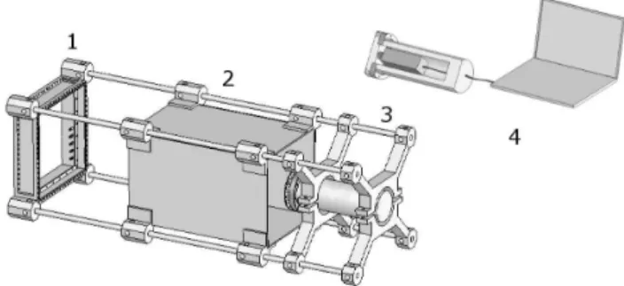
Fig. 1. Schematic illustration of the Bubblemeter: A homoge-neous high intensity light source combined with a power pack (De-vice 1) illuminates the field of observation. A box (De(De-vice 2) filled with clear water reduces water turbidity within the optical path. A high speed camera inside a pressure housing (Device 3) records se-quences of bubble images which rise in the sample area between Device (1) and (2). Data sequences are transferred to a laptop PC (4) for further analysis.
In summary, the camera system, hereafter referred to as “Bubblemeter”, is designed to be deployed and recovered from the deep sea using a remotely operated vehicle. It con-sists of a state-of-the-art high-speed camera providing high time and spatial resolution. The required intensive illumina-tion is achieved by an innovative LED light source. The post-processing procedures and bubble analysis is accomplished by an automated routine capable of identifying bubbles and measuring key features like vertical bubble speed and bubble dimensions. These parameters are essential in determining the liquid-gas mass exchange at the fluid interface. More-over, images with very high time resolution of methane bub-bles may give new insights to possible hydrate skin forma-tion. The Bubblemeter development is a three stage process. It is split into a validation and surface supplied deep-sea test-ing phase. The third stage consists of a system modification towards an autonomous operation. Here, we report on the first two stages of development.
2 Materials and Procedures
2.1 Bubblemeter design and components
The camera system consists of four components as illustrated in Fig. 1: The illumination and power storage unit (Device 1), water box (Device 2), high-speed camera (Device 3) and the data storage unit (4). The total mass of 60 kg exhibits a neg-ative buoyancy of 200 N in fresh water. The overall dimen-sions are 140 cm×50 cm×50 cm.
laboratory version for shallow water applications can be de-ployed to a water depth of 2 m, restricted only by the ca-ble length between camera and laptop. Longer caca-bles may be used but require additional shielding due to changes in the self-inductivity while submerged. The deep-sea non-autonomous version of the Bubblemeter consists of the same components as the laboratory version with only two differ-ences. The camera running on an autonomous mode can be triggered only once per dive. Secondly, the switch must be triggered by a ROV manipulator externally. In the final stage of development, the major difference to previous versions will be the control and data storage unit which will be ad-ditionally incorporated into the pressure housing. This unit will allow triggering of camera and illumination in preset fre-quencies and storing recorded images. In order to preserve energy, the control unit will set the system to standby while it is not in record mode.
Illumination: Arguably, the light source is the heart of ev-ery image processing tool. Gradients in background intensity require complex filters and computing time in order to extract bubble objects from their surrounding. A homogenously il-luminated field-of-view simplifies any segmentation strategy. Fast moving objects like bubbles require high shutter speeds and a small camera aperture. Therefore, high light intensi-ties are mandatory in order to minimize motion blur to less than 2 pixels. Also small size, low weight and low power uptake are general requirements for ROV-operated as well as autonomous underwater tools. As a result, a novel high in-tensity light source made out of LEDs was developed to meet all requirements above.
The novel light source developed for the Bubblemeter em-ploys LEDs that densely cover a square area of 30 cm×30 cm and act as point sources of light. The wavelength is Gaus-sian distributed with its peak atµ=524 nm and a deviation ofσ=10 nm. A 3 mm thick screen made out of polyethy-lene diffuses the led spots and creates a homogeneous back-ground. In air, the field of observation can be illuminated with a homogeneous light intensity of 60 Klux. The power consumption is 170 W at 12 VDC which is supplied by a 10 Ah built-in Lithium-Polymer rechargeable battery pack. In this configuration, the energy capacity is sufficient in il-luminating the field of observation approximately 60 times under laboratory conditions. Each interval lasts 10 s. Due to the fact that the required voltage for the LED configuration can only be provided for a fraction of the total battery capac-ity, this large margin was chosen, also taking into account varying discharge characteristics for low temperatures occur-ring at deep-sea sites. The illumination housing is designed to accommodate a 40 Ah battery pack of the same make. Po-tentially, this increases the number of activations to approxi-mately 240. The housing is pressure compensated and filled with silicone oil. This enables quick transport of heat en-ergy to the surfaces, as well as a thin walled and lightweight housing.
Fig. 2. Left; Inhomogeneously illuminated grey scale image. Pa-rameter “a” and “b” denote the major and minor axis of a best fit ellipse encircling the bubble. The white scale bar has a length of 10 mm. Centre; Bubble segmentation using the threshold method. Right; Bubble segmentation applying the edge detection method. The edge detection method results in an accurate representation of the bubbles and is, in addition, less sensitive to inhomogeneous background illumination compared to the threshold method.
Frame: The frame consists of 4 stainless steel bars and act as a guide rail. It accommodates the pressure container, the clear vision box and the illumination device. The size was chosen considering the technical feasibility in a remote op-erated vehicle deployment as well as ensuring that even fast moving bubbles can be tracked for a sufficiently long time. Due to the adjustable design, the length of the system may be varied as appropriate. For turbid waters, a clear vision box may be used. This box, filled either with clear saline or non-saline water, reduces the volume of potentially tur-bid water in front of the screen, thus, enhancing the image contrast. Normally the clear vision box would be filled with surface water on site. Alternatively, the box may be filled with transparent oil in order to increase buoyancy.
2.2 Image processing and analysis
An automated routine is needed in order to process and anal-yse images with statistically relevant numbers of gas bub-bles within reasonable time and accuracy. The algorithm must perform simple and fast segmentation as well as fea-ture extraction. Furthermore, the algorithm must be capa-ble of tracking individual bubcapa-bles and store the results in a useful format. Therefore, the key features of the presented routine may be summarized by isolating bubbles from the background and determining their position and bubble sizes. In a second step, the routine can track bubbles in successive frames, analyse and store the data in a cubic matrix. The following paragraph describes the new concept in detail.
In general, segmentation is the process of discriminating objects of interest from the remaining image. In this case, it is the process deciding whether any image pixel belongs to a bubble or is part of the background. In the segmentation strategy followed in this study, a “Canny” filter is used for grey value images. It compares the value of each pixel rela-tive to the values of its neighbourhood (Canny, 1986). When the grey value gradient between two adjacent pixels is larger than a preset level, the pixel is set to binary 1, otherwise it is set to binary 0. As a result, edges are created around objects. The major advantage of using the edge detection strategy rather than applying a simple grey value threshold is illus-trated in Fig. 2. The edge detection identifies the bubble boundaries even in inhomogenously illuminated areas. Fur-thermore, it can also be applied to images with steadily de-creasing light intensities. In contrast, the image that is seg-mented using a grey value threshold shows some degenera-tion in bubble shape. Also the background may be misinter-preted due to the inhomogeneous background illumination.
However, there are two disadvantages in using the edge detection strategy, which we consider as minor compared to the improvement of the method. One disadvantage is the increased computing time compared to using the intensity threshold. The computing time varies between milliseconds and seconds and depends on the image size. The second dis-advantage is a systematic enhancing or suppressing of bub-ble boundaries. Depending on the edge threshold the bubbub-ble grows or shrinks during segmentation. This can be compen-sated using dilation and erosion filters which add or subtract pixels to the boundaries of objects. Yet, applying additional morphological filters requires extra processing time and adds on to the first disadvantage. The final output is a binary im-age which is an isometric mapping of the original imim-age.
In general, feature extraction is the process of reducing the object information to the relevant key features of inter-est. Here, the bubble size as well as the centre of the bub-ble area is determined using the Matlab® routine “Region-props”. These values are based on an elliptical best fit as exemplified in Fig. 2.
In a second step, bubbles are tracked in successive frames and their rise velocities are computed. This is realized using
the following assumption: the distance that a bubble has trav-elled in two successive images is smaller than the distance to its closest neighbour. This assumption is valid except for overlapping bubbles, very high bubble concentration and for low acquisition frequencies where travel distance is greater than neighboured bubble distance. Objects that do not move or sink are automatically excluded.
Finally, the vertical flux of bubbles through the sample vol-ume is calculated. Since bubbles are imaged and measured multiple times during their rise, each measurement has to be weighted by a weighting factorη. It represents the number of measurements made of a single bubble during its rise through the sample volume and is determined by the following equa-tion:
η=(Y−2·h)
Dz
(1) whereDzis the vertical shift of an individual bubble.Y rep-resents the image size in vertical direction andhthe vertical bubble diameter. For example, in order to count bubbles, each measurement results in an increase of the bubble num-ber by1η. Afterηmeasurements of the same bubble, its bub-ble number has risen to ηη=1 while the bubble has left the image. Therefore, intermittent errors such as bubble overlap or unsuccessful bubble assignment contribute by a factor η1 to each measurement only. At the same time, the recipro-cal factor may also be interpreted as particle flux through the horizontal cross-section. Thus, the higher the image acqui-sition frequency and the lower the rise velocity to the limit where motion can no longer be detected, the largerηis, the smaller is the contributing error. This weighting factor also applies to variations in bubble numbers and rise speed.
3 Assessment
Three key experiments were conducted to test the concept of the gas quantification system. Firstly, the reliability of the automated segmentation routine and bubbles size measure-ment was tested. The results showed that the system maps bubble images onto binary images isometrically. Secondly, parameters for assessing the bubble assignment ability were introduced. It shows that at least 75% of the bubbles are as-signed correctly. Thirdly, a series of calibrated gas flux mea-surements between 2 L/min and 12 L/min were performed. The results reveal a linear dependence between the flux de-termined by the Bubblemeter and the actual gas flux. The system is able to determine gas flow rates in the order of magnitudes of mL/min up to an amount of 10 L/min. The error is typically in the scale of 5–10% for low flow rates and ranges to a maximum of 33% for high flow rates.
3.1 Size mapping
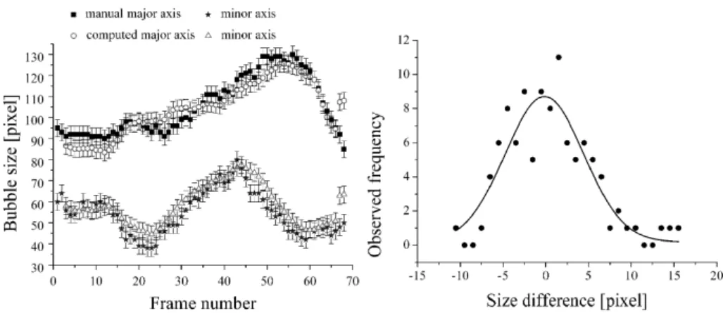
Fig. 3.Left; Comparison between manually measured and computed bubble sizes. The computed major axis (circle line) and the computed minor axis (triangle line) correspond mostly within the error of±4 px with their manually measured counterparts. Right; The frequency distribution for size differences between manually measured and computed axes lengths can be approximated using a Gaussian fit. The error bars are consistent with the standard deviation ofσ=4,6±0,6 px.
approach. The bubbles were elliptically shaped. The di-ameter of their major axis ranged between 1 to 20 mm (10 to 200 pixels). Figure 3 (left) illustrates the size evolution of one representative bubble. The bubbles oscillating dur-ing ascend produce a size variation of both axes. Within the uncertainty of measurement, there is generally a good corre-spondence between the values based on the automated esti-mation and those that were determined manually. In the case of the manual size measurement, the uncertainty of±4 px comprises of±2 px for the edge determination and±2 px for estimating the major and minor axis orientation respec-tively. In the case of the automated measurement the uncer-tainty of±4 px constitutes of±2 px for detecting the blurred edge of the bubble boundary. An additional uncertainty of±2 px takes possible edge enhancement due to the edge detection process into account. Quantifying the accuracy between manually and automatically measured bubble sizes yields a frequency distribution which is shown in Fig. 3 (right). The difference in bubble size determination is small with a median ofX¯ = −0,15 px. The standard deviation of
σ=4,6±0,6 px is consistent with the measurement uncer-tainty illustrated as error bars in Fig. 3 (top).
3.2 Bubble assignment
A strategy has been developed assessing how successful bub-bles have been tracked by the automated image analyses. Us-ing the least distance assumption, it was manually verified that individual bubbles can be tracked in successive frames. In a second step, the parameterβ was introduced to quan-tify the rate of successful assignments for approximately 106 bubbles.
In the initial experiment, 23 single bubbles were tracked at a flow rate of 1 L/min and their sizes were analysed. The gas flux was created using a pump for aquarium purposes and led into a bare hose. The gas flux was calibrated by
mea-suring the time required to fill a volume of 250 ml. The ori-fice was 3 mm in diameter. It was aligned horizontally in the setup and produced bubbles with irregularly shaped and os-cillating bubble surfaces. The major axis diameters varied between approximately 7–12 mm (70–120 pixels). The bub-bles did not overlap and maintained a distance of 6–12 mm (60–120 pixels) to their predecessors. The automated assign-ment method resulted in 1150 size measureassign-ments. However, the algorithm failed twice to successfully track the individual bubble in successive frames. While there is a gradual change in the sizes of the axis between successive frames (see for example Fig. 3 left), assignment errors appeared as a simul-taneous and unsteady break in the measurement of both bub-ble axes. This indicates that a different bubbub-ble of different major and minor axis size had been erroneously tracked. The mistaken assignment can be explained by shape oscillation. In rare cases, sporadic shape deformation can cause a nega-tive rise of the centre of the bubble area. This neganega-tive rise excludes the bubble from assignment momentarily.
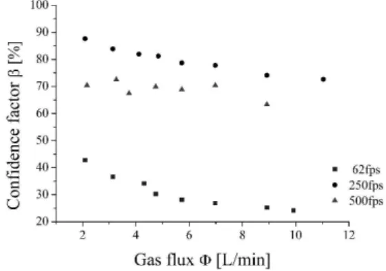
Fig. 4.The ratioβshows the flux dependent accuracy of bubble as-signment with an asas-signment of 85% decreasing to 75% for 250 fps. At 500 fpsβremains approximately constant for all flow rates while for 62 fps most of the bubbles cannot be assigned successfully.
In a next step, the sensitivity of the assignment procedure was tested for a range of gas flow rates that may be encoun-tered in the natural system. Additionally, the speed of image acquisition varied between 62, 250, and 500 fps to investi-gate its influence on bubble assignment ability. A hole was drilled into a block of plastic and connected to a pressure vessel. Its orifice was 1 mm in diameter pointing vertically upwards. An experiment with calibrated flow rates ranging between 2 L/min and 12 L/min was set up and the parame-ters were intentionally set to represent a worst-case scenario. This caused rising bubbles to overlap, coalesce and break up again. The flux was determined using a flow meter (Fischer & Porter; Model NR FP1/4−20 G5) and controlled by mea-suring the time that was required to fill a volume of 2 L. Each flow rate was recorded with 500 fps, 250 fps and 62 fps. In each sequence, the total object numbers ranging from 105 for 2 L/min up to 107for 12 L/min were recorded.
Figure 4 shows β against gas flux 8for three different recording frequencies. The figure illustrates the highest as-signment factor was achieved at recording frequencies of 250 fps. Neither higher nor lower acquisition frequencies in-crease the assignment factor. At 62 fps the number of suc-cessful assignments is below 45% at low flux rates and de-crease further with increasing flux. This poor assignment ability can be explained by the fact that the least distance as-sumption is not valid anymore. The distance bubbles travel in between successive frames is larger than the distance of neighbouring bubbles. This is even more obvious at high flow rates which results in high bubble population densities. At 500 fps the assignment factor remains approximately con-stant for all flow rates with a value of about 70%. At these high acquisition frequencies, the observed bubbles move in average between 2 pixel and 6 pixel per frame. Therefore, the least distance assumption remains valid. In addition, the bubble shape remains nearly identical. However, bubbles that do not rise at all in successive frames are excluded from the assignment in order to prevent misinterpretation of
for-eign objects. At acquisition frequencies of 250 fps, the ratio decreases steadily from approximately 85% for 2 L/min to 75% at 12 L/min. This trend might be explained by the fact that with increasing fluxes the numbers of bubble in each frame increases and that, consequently, more bubbles over-lap, which leads to decreasingβ values. This statement is supported by the observation made in the previous experi-ment with single bubbles at 1 L/min. Out of 1150 assign-ments only two were corrupted yielding a ratio ofβ=99.8%. In conclusion, 250 fps has been found to be the optimum recording frequency with an assignment factor in the range of 85% to 75%.
3.3 Flux measurement
Lab experiments were conducted in order to test how good the Bubblemeter and the subsequent automated analyses ac-tually measure the bubble flux. The result of the automated analyses shows a linear dependency between the measured and the actual bubble flux. This implies that the calculation routine systematically overestimates the actual flux by a con-stant factor. It can be shown that the overestimation is caused by irregular bubble shapes which are predominately the re-sult of a two dimensional image projection of the observed volume.
A laboratory experiment was set up to record gas flows and to compute the image data obtained. A water tank 1 m×1.5 m×1 m in dimension was filled with tap water at room temperature (T =20◦C). Three upward pointing
noz-zles with 5 mm, 3 mm and 1 mm in diameter were placed 0.7 m below surface. The Bubblemeter was submerged just underneath the surface. The image size obtained was 30 cm with the screen at the top 5 cm below surface. The plume rose in the centre of the observation volume and was completely imaged. The mean distance between plume and camera was 0.8 m yielding a resolution of 319±17 µm/px. The recording frequencies were set to 500 fps and 250 fps. Each sequence contained 1000 frames and recorded a time interval of 2 s and 4 s respectively. High pressure Scuba tanks provided the gas supply via low pressure hoses. The gas pressure was reduced to constant intermediate pressure while a fine control valve was used to adjust the appropriate gas flow. The flow rate was monitored using a calibrated flow meter tube (Fischer & Porter; Model NR FP1/4−20 G5). Eight measurements in the flow range between 2 L/min and 12 L/min were taken for each diameter and each of the recording frequencies. All measurements were in the flow regime of bubbly jet streams. Shortly after detachment, every second bubble accelerated within the wake of their predecessors and penetrated them. During the ascent, bubbles broke up and occasionally formed agglomerates again. The observed shapes can be classified as small spherical bubbles, bigger ellipsoids to even larger spherical cap-shaped bubbles.
Fig. 5.In both models the computed flux can be linearly correlated to the physical flux. The ellipsoidal model yields an overestimation factor of 4.8±0.6 while the sphere model yields an overestimation of 2.2±0.3.
Table 1. The frequency combined mean slope for the ellipsoidal model yields a systematic overestimation of 4.8±0.6 while the sphere yields 2.2±0.3.
Model Frequency (fps) B R2
Ellipsoidal 250 4.2 0.98850
500 5.4 0.95219
Sphere 250 1.9 0.90465
500 2.4 0.99105
assumes an ellipsoidal shape using the bubble length and width as major and minor axis while the bubble depth is as-sumed to be identical to its width. Another model uses an equivalent area approach: the sphere radius is determined by a circular area which is equivalent to the cross-section area of the particular bubble. For simplicity, this model will be referred to as the sphere model in the following. Both ap-proaches have been applied in order to compare model pend-ing discrepancies but they have been found to be equally valid, as shown further below.
Figure 5 shows a linear correlation between actual and es-timated flux resolved for each frequency and model. Table 1 presents the essential linear least square fit parameters for both models and for 500 fps and 250 fps, respectively. Within an error of 33% each model shows a frequency independent linear correlation between estimated and actual flux. 3.4 Model evaluation
Both models show a systematic overestimation of the mea-sured gas flux. In order to investigate the origin of the over-estimation, the volume of single bubbles and bubble clusters have been estimated manually. The deviation of 4.8 for the ellipsoidal model and 2.2 for the sphere model could be re-produced indicating the source of error to be model induced. In addition, the impact of large bubble clusters to the total
Fig. 6.The compositions of various bubbles merging and overlap-ping each other create bubble clusters. The volume of a best fit ellipse is larger than the actual gas volume. These clusters carry the majority of gas dominating the overestimated computed flux. The white scale bar below is 1 cm long.
gas volume was examined. The volume shows a strong de-pendency on theses clusters emphasizing the model induced overestimation.
The volumes of ten single bubbles oscillating moderately have been compared with the automatically estimated vol-umes using the ellipsoidal as well as the sphere approach. The ratio of the estimated versus actual volume is denoted as
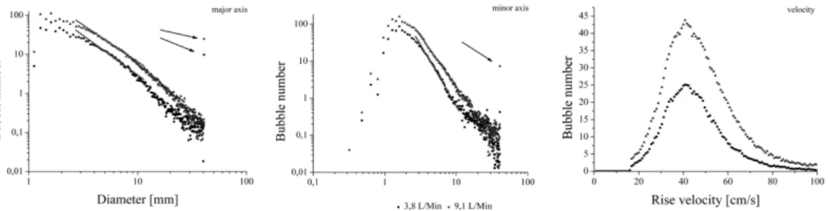
Fig. 7.Bubble size distributions for the major axis (left) minor axis (centre) and rise velocity distribution (right) for 3.8 L/min and 9.1 L/min. An increased gas flux yields increasing bubble numbers while the bubble size and rise velocity distribution remains constant. Note the single peaks at the cut off end of the distribution. These represent large bubble clusters. They are not well approximated by the model and are predominantly responsible for flux overestimation.
Table 2.The gradients for the high and low flow distribution can be approximated using similarly valued parameters. This holds for the major axis as well as for the minor axis distribution in Fig. 7.
Axis Flux (L/Min) α γ R2
major 3.8 2.5 −2 0.98107
9.1 2.7 −1.9 0.99095
minor 3.8 3.1 −3.3 0.99182
9.1 3.0 −2.7 0.99618
3.5 Volume distribution
The apparent difference between the ellipsoidal and the sphere model is most pronounced for large irregular shaped bubbles as well as for bubble clusters. Due to lack of ro-tational symmetry and information on the third dimension, the assumption that bubble width equals bubble depth is not readily valid for large bubbles and clusters. However, these large bubbles and clusters are predominantly responsible for the volume overestimation during automated flux analyses. The peak values at the cut-off end of the size distribution in Fig. 7 indicate that large bubbles and clusters represent a small minority in the size spectrum only. Yet, the automated flux estimation is influenced considerably by the model pend-ing overestimation suggestpend-ing only few mega bubbles carry a significant amount of volume.
In order to determine the impact of bubble clusters on the total volume, the size information in the class with the largest sizes (Fig. 7) was extracted. The ratios between bubble umes in this large-size class with respect to the total gas vol-ume indicate the volvol-ume impact of bubble clusters. The re-sults show that less than 1% to 3% of all bubbles carry be-tween 30% and 90% of the total gas volume. Consequently, due to the limited approximation of artificial bubble clusters their systematic volume overestimation transfers onto the to-tal gas volume computation. This also implies that the mod-els used to estimate the volume are valid for 97%–99% of the observed bubbles. This is an important result and confirms the accuracy of the computed size distribution spectra.
3.6 Frequency distributions
Bubble size and rise velocity are two important parameters for mass transfer in gas-liquid two-phase flows such as bub-ble plumes. Gas exchange is dominated by the interfacial bubble area as well as by the time the surface is exposed to the liquid phase. It is, therefore, essential to test the system capability to determine these parameters within the specified accuracy. For example, Fig. 7 shows the major and minor axis frequency distribution as well as the rise velocity fre-quency distribution at flow rates of 3.8 L/min and 9.1 L/min, respectively. The orifice diameter was 5 mm and the acqui-sition frequency 250 fps. The size distribution can be ex-pressed in a power function where Nb is the bubble number,
αis a general constant andγ a negative power constant.
Nb=α·Dγ (2)
Using the log representation and the rule log(10α×Dγ)= α+γ×logD, Eq. (2) enables us to determine the power con-stant by means of the slope of a linear least square fit of the distribution.
Table 2 shows the linear least square fit parameters for the bubble size distributions shown in Fig. 7 (left) and Fig. 7 (centre). For each axis, the size distribution for high and low flow can be approximated by similar linear functions. Conse-quently, the size distribution does not change for bubbles in between the two measured flow regimes. An increased flow primarily causes increased bubble numbers for the selected flow rates.
The same observation can be made for the velocity dis-tribution in Fig. 7 (right). The data are displayed in a linear scale representation. An increased flux causes increased bub-ble numbers instead of an increased rise velocity. The mean velocity for 3.8 L/min is given by v=42.3±0.2 cm/s and
Table 3.For each bubble diameter the terminal velocities by Haberman & Morton2is added to the fluid velocity determined by Whalley & Davidson1and compared with the measured values.
Bubble size Bulk flow1 Terminal velocity2 Cumulative velocity Measured rise velocity
(mm) (cm/s) (cm/s) (cm/s) (cm/s)
1.7 22 19 41 40.7
2.7 22 44 44.6
3.5 24 46 42.7
1.7 30 19 49 42.2
2.7 22 52 45.0
3.5 24 54 43.0
compared for 3.8 L/min and 9.1 L/min. The bubble sizes were chosen for their local maxima in a two dimensional representation of the size distribution. The result is only a slight increase in rise velocity, varying from 1.5±0.2 cm/s for 1.7 mm, 0.4±0.2 cm/s for 2.7 mm and 0.3±0.2 cm/s for 3.5 mm. These data support the observation made earlier. The bulk flow velocity does not increase with the same rate as the gas flux increases.
A simple approach to this problem is a two-phase model with a non-interacting gas and liquid phase. Here, the gas bubbles rise within a bulk fluid driven by gravity only. The terminal velocity is described as the rise velocity of single bubbles in absence of bulk flow. The potential energy re-leased by the bubble during ascent is converted to kinetic en-ergy of the bulk fluid. The fluid velocity is superimposed by the terminal velocity yielding a total vertical bubble velocity. For simplicity, the total vertical bubble velocity has been re-ferred to as bubble rise velocity in this work. Haberman and Morton investigated the terminal velocity for air in tap water (Haberman and Morton, 1953). They measured terminal ve-locities between 19 cm/s and 24 cm/s for the specified bubble diameters. Figure 8 shows the measured rise velocities for each diameter together with the terminal velocity measured by Haberman and Morton. The difference between bubble rise velocity and terminal velocity may be assigned to the upwelling effect of the gas flux causing bulk flow.
The concept of a superficial gas velocity is used in order to quantify the impact of the gas flux to the bulk fluid momen-tum. The gas velocity is the speed of the gas-liquid interface displacing the fluid within a pipe. For a cross-section area of approximately Across=500 cm2 this yields a gas veloc-ity ofvg=0.13mm/s andvg=0.3mm/s for 3.8 L/min and 9.1 L/min, respectively. Whalley and Davidson investigated the correlation between bulk fluid velocityvf l and gas ve-locityvg which causes the bulk flow (Whalley and David-son, 1977). The results yielded that fluid motions varied betweenvf l=22cm/s forvg=0.1mm/s andvf l=30cm/s for vg=0.3mm/s. The measurements were carried out in tanks where the height to width ratio was smaller than one and where wall effects could be neglected. Conclusively, the
Fig. 8. The measured rise velocities for bubbles with major axis diameters of 1.7 mm, 2.7 mm and 3.5 mm are plotted for each flow rate. The rise velocity error is given by 2 mm/s and equals the size of the plotted objects. Additionally, the terminal velocity measured by Haberman and Morton is shown. The difference between bubble rise velocity and terminal velocity may indicate liquid bulk flow.
measured rise velocities ofv=42.3 cm/s andv=43.4 cm/s are in good agreement with the combined results of Whalley & Davidson and Haberman & Morton which are displayed in Table 3.
from the same water source and, therefore, showed the same effects.
Another point of interest is the increase of bubble rise ve-locity for different flux rates. Figure 7, Fig. 8 and Table 3 indicate, that the rise velocity increases between 42.3 cm/s and 45.0 cm/s opposed to the theoretically anticipated val-ues of 49 cm/s and 54 cm/s. Therefore, a new approach is needed since measuring errors can be excluded as shown above. Instead of dealing with two phases separately, the new approach must consider the interaction of the liquid with the gaseous phase. The observed assumingly reduced rise velocity may be explained by including turbulences, shear stress, momentum transfer and energy dissipation (Brauer, 1979). For low gas contents small bubbles up to approxi-mately 1.5 mm in diameter rise rectilinear. Above 2.0 mm bubbles tend to rise on helical pathways. However a further increased gas contents causes bubbles to rise increasingly rectilinear again. (Miyahara and Yamanaka, 1993). As the horizontal velocity component decreases, the vertical com-ponent increases. This effect is more pronounced for small bubble diameters and it decreases for larger bubbles. There-fore, bubbles in bubbly swarms or jet streams rise faster than single bubbles measured by Haberman & Morton. The ten-dency towards rectilinear bubble motion is influenced by an increasing turbulent flow field around the bubbles.
These instantaneous fluctuations cause bubble deforma-tions which themselves react to the perturbation by produc-ing chaotic and highly variable flow fields organized as ed-dies (Serizawa et al., 1975; Schl¨uter, 2002). With increasing gas contents, the bubble-induced turbulences become more dominant resulting in an increased flow resistance. Eddies also increase the exchange of momentum between the bulk fluid and its boundary, causing a reduced velocity gradient profile (Brauer, 1971 and 1979).
Thus, the barely increasing observed bubble rise velocity in Table 4 can be explained by an eddy induced increased flow resistance together with a decreasing velocity gradient profile in the bulk fluid.
3.7 Error estimation and impact
The error for gas flux determination is a combination of opti-cal resolution, bubble segmentation, assignment ability and model accuracy. Optical resolution and bubble segmenta-tion errors remain constant for all flow rates. The assignment ability and the model accuracy, however, vary with the flux related bubble population density. The latter two dominate the absolute error significantly. In order to discuss the er-ror estimation, the end members in the bubble-size spectrum may be distinguished and discussed separately.
Most numerous were those bubbles with a small bubble size of about 3 mm (ca. 10 px) in diameter. For this case, the optical uncertainty ofσ=17 µm/px causes a volume error of 16%. The segmentation error of±4 px contributes with up to 100%. Because small bubbles can be considered
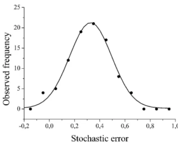
spheri-Fig. 9.The frequency distribution for the relative variance between measured and computed flux is illustrated. Using a Gaussian fit the stochastic error of the computed flux can be approximated. The median error of 33% corresponds to the evaluated theoretical error of 34%.
cally shaped, the model error is negligible. The error caused by unsuccessful bubble assignment can only be estimated. As mentioned above, an unsuccessful assignment excludes the bubble volume momentarily from computation. An up-per error limit is given by 100% –βindicating the proportion of unsuccessful assignments. Most of the failed assignments will concern small bubbles. Therefore, it is assumed that the assignment error is in the range of 15%–25% for sequences with an acquisition frequency of 250 fps. Summation over all values above yields a maximum error of 141%. For flux determination, this value must be weighted with the relative volume transported through small bubbles which is as low as 10%. This may lead to a minimum flux error of approxi-mately 14% caused by small bubbles.
respect to the overestimation factor. The same result may be obtained for the sphere model by dividing the deviation of±0.3 with respect to the overestimation factor of 2.2. This results in an error of 13%. Summing over the errors of the second bubble class and weighting with the relative volume yields an error of approximately 34%. This estimated theo-retical value has been verified experimentally.
After correcting the automatically estimated flux data for the systematic overestimation, the relative variance between actual and estimated flux was determined. The cumulative result for 500 fps and 250 fps including both models is illus-trated in Fig. 9. The random errorEin flux determination can be approximated by a Gaussian fit. The median error is
¯
E=0.33 with a standard deviation ofσ=0.31. These values are in good agreement with the anticipated theoretical error of 34%.
The error in bubble rise velocity may be estimated as fol-lows. For the uncertainty in rise velocity, error propagation may be applied. The centre of the bubble area may be deter-mined within the limit of 0.5 pixel. This value is justified by the continuous Gaussian shape distribution in Fig. 7. The re-sult of multiplying this value with the differential resolution yields a rise velocity uncertainty of 2.1 mm/s.
4 Discussion
The objective of the work presented is to introduce a new de-sign for gas quantification under water. One key element of the system is the image analysis routine. It could be shown that bubbles are isometrically mapped onto binary images. Test procedures were introduced proving the system’s ability of successfully tracking bubbles within the volume of obser-vation and to quantify the rate of successful bubble assign-ments. Laboratory measurements indicate a linear depen-dency between estimated and actual gas flux. A systematic overestimation of 4.8±0.6 was calculated for the gas flux using an ellipsoidal model. For the sphere model, the over-estimation was 2.2±0.3. The initial objective has been met under laboratory condition. The optical system is capable of quantifying gas flow rates in the range between 2 L/min and 10 L/min with an uncertainty of 33%. The verification pro-cess has identified limitations of the new gas quantification system.
4.1 Limiting parameters
The performance depends on three primary parameters, such as acquisition frequency, image size as well as bubble pop-ulation density. Other parameters such as bubble size, rise velocity, bubble shape and sequence length can be derived from those mentioned above.
Acquisition frequency: Frequencies which are too high cause bubble exclusion due to momentarily nil or negative rise velocities. On the other hand, frequencies that are too low, i.e. 62 fps inhibit successful bubble tracking. Therefore,
an upper limit of 500 fps for analysing bubble plumes can be set. For the low frequency side, the bubble population density must be taken into account. The higher the popula-tion density, the shorter the mean distance between the near-est neighbours. Consequently, the higher the acquisition fre-quency must be. At flow rates between 2 L/min and 10 L/min 250 fps was identified as ideal recording speed.
Image size: The minimum vertical image size has been found to be 150 px. This is approximately three times the size of the vertical dimension of the largest bubbles observed. Increasing the image size from 150 px to 500 px improved the number of successful bubble assignments steadily. Above 500 px the rate of successful assignment remained constant. It is, therefore, suggested that for further applications, the dimension of vertical image size is ten times the height of the largest observed bubble, in this case 500 px.
Bubble population density: Unlike frequency and image size, this natural parameter can not be controlled in deep-sea applications. Essentially it affects bubble agglomeration and formation of two dimensional projected bubble clusters. Generally, flow rates of 2 L/min and above result in bubble populations densities which cause significant bubble agglom-eration and formation of bubble clusters on the images. Flux computation is then only possible using predetermined cali-bration factors.
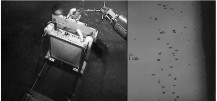
After having completed stage 1 of the development pro-cess, the next step in the assessment process is to verify that the system can be deployed under deep-sea conditions. The Bubblemeter was, therefore, deployed to 1023 m water depth during the M74/3 research expedition at the Makran accre-tionary prism in November 2007. During that cruise, the remote operated vehicle (ROV) ‘Quest’ was launched from the research vessel R/V Meteor in order to investigate active gas seeps offshore Pakistan. The Bubblemeter was mounted onto the front porch of the ROV. The camera was operated in the built-in autonomous mode and synchronised with the illumination device. The Bubblemeter was positioned at an active bubble stream (Fig. 10, left). The camera and light were turned on using the ROV manipulator. A two-second sequence with 1000 single images was recorded at a fre-quency of 500 frames per second. Figure 10 (right) shows one image taken by the high-speed camera. The in situ flux was determined to be 140±10 mL/min. Due to a small bub-ble population density and well-approximated bubbub-ble shapes, the error was primarily caused by optical resolution uncer-tainty.
5 Comments and recommendations
Fig. 10. Left photo taken by the ROV operational camera; ©MARUM. The Bubblemeter is positioned and ready to be trig-gered by the ROV manipulator. Right: Gas bubbles rise in between the camera and the illumination device. The black bar positioned at the centre left is scaled to 1 cm.
taken at intervals of about 2 h or less in order to obtain suf-ficient samples within the tides. The system is intended to cycle between a recording, data transfer and stand-by mode. To achieve this goal, three key elements have to be added to the current design.
Camera: The camera specifications have been identified during the test procedures. The camera must record 250 fps at VGA resolution. The camera interface is ideally GENI-CAM conform and has a GB Ethernet connection. Cameras with these specifications are available on the market and have a power consumption of 5 W.
Control unit: An embedded PC system must be designed to control the camera, the illumination device and to transfer the image data onto a memory device. The unit will reach a power consumption of 30 W during peak performance. The external memory device will have a capacity of 120 GB and be able to store about 100 sequences. Limited memory space is the restricting resource of the autonomous device.
Power: During the last deployment, valuable data on power consumption of the utilized 10 Ah Li-Po battery pack has been obtained. Particularly, temperature reduces the nominal power capacity. In the laboratory, the capacity was sufficient for 60 test runs each 10 s of duration. Power consumption during deep-sea deployment suggests that only 20 cycles would have been possible in situ. Therefore, it is planned using a 40 Ah Li-Po battery pack and reducing the interval to 5 s. Theoretically, this enables 80–160 sequences to be illuminated. The control unit is intended to run inde-pendently on a 10 Ah Li-Po battery pack. This will allow the unit to run a minimum of 1 h at peak performance in situ.
Improvements on behalf of camera, power- and informa-tion storage equipment will lead to a monitoring device with an anticipated performance of 100 sequences in 15 min in-tervals over a period of 24 h. Although memory capacity is the limiting factor for the deployment duration, the system will not process the image data in situ. There are two reasons against it. Firstly, any optical misinterpretation such as ma-rine snow or barnacles can not be identified without the raw
images. Secondly, raw images may be of great value when examining the bubble-fluid interface within the hydrate sta-bility zone.
Some valid critical aspects of the system setup are its lim-ited field of observation and lack of quantifying flux rates over a large scale seep field. Also the device must be po-sitioned precisely on top of an active seep. The purpose of the present device is local high resolution imaging of single gas vents. Large scale quantification may be achieved using additional acoustical backscattering methods for example.
Acknowledgements. We would like to thank Ira Leifer and Aneta Nikolovska for their expertise during numerous helpful dis-cussions. We also thank and appreciate the constructive comments made by the reviewers and the guest editor. Special thanks go to Wilfried Sch¨utz and Uwe Grossmann for their continuous encour-agement. We would like to thank the crew of the research vessel R/V Meteor as well as the ROV operators whose great efforts turned the “Bubblemeter” deployment into a success.
This research was part of “MarTech” and primarily funded by the Helmholtz Association as part of the “Impuls- und Vernet-zungsfonds”. Furthermore, the study was partly funded by the DFG-Research Center/Excellence Cluster “The Ocean in the Earth System”. The project received further helpful support by the Institute for Marine Resources, Bremerhaven, and ERDF (European Regional Development Fund).
Edited by: G. Griffiths
References
Agrawal, Y. C. and Pottsmith, H. C.: Autonomous Long-Term in situ Particle Sizing Using A New Laser Diffraction Instrument, OCEANS, 5, 1575–1580, 1989.
Belcher, E. O.: Quantification of Bubbles Formed in Animals and Man During Decompression, IEEE Trans. Biomed. Eng. 27, 330–338, 1980.
Brauer, H.: Grundlagen der Einphasen- und Mehrphasen-str¨omungen, Verlag Sauerl¨ander, Aarau und Frankfurt am Main, 1971.
Brauer, H.: Turbulenzen in mehrphasigen Str¨omungen, Chem.-Ing.-Tech., 51, 934–948, 1979.
Boetius, A., Ravenschlag, K., Schubert, C. J., Rickert, D., Wid-del, F., Gieseke, A., Amann, R., Jørgensen, B. B., Witte, U., and Pfannkuche, O.: A marine microbial consortium apparently me-diating anaerobic oxidation of methane, Nature, 407, 623–626, 2000.
Canny, J.: A Computational Approach to Edge Detection. IEEE Trans., Pattern Analysis and Machine Intelligence, 22, 679–698, 1986.
Deane, G. D. and Stokes, M. D.: Scale dependence of bubble creation mechanisms in breaking waves, Nature, 418, 839–844, 2002.
de Vries, A. W. G., Biesheuvel, A., and van Wijngaarden, L.: Notes on the path and wake of a gas bubble rising in pure water, Int. J. of Multiphase Flow, 28, 1823–1835, 2002.
Eisma, D., Schuhmacher, T., Boekel, H., van Heerwaarden, J., Franken, H., Laan, M., Vaars, A., Eijgenraam, F., and Kalf, J.: A camera and image-analysis system for in situ observation of flocs in natural waters, Neth. J. Sea Res., 27, 43–56, 1990. Greinert, J. and N¨utzel, B.: Hydroacoustic experiments to establish
a method for the determination of methane bubble fluxes at cold seeps, Geo. Mar. Lett., 24, 75–85, 2004.
Haberman, W. L. and Morton, R. K.: An experimental investiga-tion of the drag and shape of air bubbles rising in various liq-uids, Report 802, Navy Dept., David W. Taylor Model Basin, 68 Washington DC, 1953.
Hornafius, J. S., Quigley, D., and Luyendyk, B. P.: The world’s most spectacular marine hydrocarbon seeps (Coal Oil Point, Santa Barbara Channel, California): Quantification of emissions, J. Geophys. Res., 104, 20703–20711, 1999.
Judd, A. G.: Natural seabed gas seeps as sources of atmospheric methane, Environ. Geol., 46, 988–996, 2004.
Karpen, V., Thomsen, L., and Suess, E.: A new ,schlieren’ tech-nique application for fluid flow visualization at cold seep sites, Mar. Geol., 204, 145–159, 2004.
Lamarre, E. and Melville, W. K.: Instrumentation for the measument of void-fraction in breakingwaves: Laboratory and field re-sults, IEEE J. Oceanic Eng., 17, 204–215, 1992.
Leighton, T. G., Ramble, D. G., Phelps, A .D., Morfey, C. L., and Harris, P. P.: Acoustic detection of gas bubbles in a pipe, Acta Acustica, 84, 801–814, 1998.
Leifer, I. and Patro, R. K.: The bubble mechanism for methane transport from the shallow sea bed to the surface: A review and sensitivity study, Cont. Shelf Res., 22, 2409–2428, 2002. Leifer, I., De Leeuw, G., Cohen, L. H., and Kunz, G.: Calibrating
optical bubble size by the displaced mass method, Chem. Eng. Sci., 58, 5211–5216, 2003.
Leifer, I. and MacDonald, I.: Dynamics of the gas flux from shallow gas hydrate deposits: interaction between oily hydrate bubbles and the oceanic environment, Earth Planet. Sci. Lett., 210, 411– 424, 2003.
Leifer, I. and Boles, J.: Measurement of marine hydrocarbon seep flow through fractured rock and unconsolidated sediment, Mar. Pet. Geol., 22, 551–568, 2005.
MacKay, R. S. and Rubisson, J. R.: Decompression studies using ultrasonic imaging of bubbles, IEEE Trans. Biomed. Eng., 25, 537–544, 1978.
McGinnis, D. F., Greinert, J., Artemov, Y., Beaubien, S. E., W¨uest, A.: Fate of rising methane bubbles in stratified waters: How much methane reaches the atmosphere?, J. Geophys. Res., 111, CO9007, doi:10.1029/2005JC003183, 2006.
Michelson, D. L., Longe, J. W., Smith, T. A., and Suggs, J. A.: A micro bubble dispersion inwater – what role in industrialwaste treatment? Proceeding of Mid-Atlantic Industrial WasteWater and Hazardous Materials Conference, 13–30, 1988.
Miyahara, T. and Yamanaka, S.: Mechanics of motion and defor-mation of a single bubble rising through quiescent highly viscous Newtonian and non-Newtonian media, J. of Chem. Eng. Japan, Tokyo 26(3), 297–302, 1993.
Nikolovska, A. and Waldmann, C.: Passive acoustic quantifi-cation of underwater gas seepage, OCEANS 2006, 1, 1–6,
doi:10.1109/OCEANS.2006.306926, 2006.
Nikolovska, A., Manasseh, R., and Ooi, A.: On the propagation of acoustic energy in the vicinity of a bubble chain, J. Sound Vib., 306, 507–523, 2007.
Nikolovska, A., Sahling, H., and Bohrmann, G.: Hydroacous-tic methodology for detection, localization, and quantification of gas bubbles rising from the seafloor at gas seeps from the eastern Black Sea, Geochem. Geophys. Geosyst., 9, Q10010, doi:10.1029/2008GC002118, 2008.
Orphan, V. J., House, C. H., Hinrichs, K.-U., McKeegan, K. D., and DeLong, E. F.: Methane-consuming archaea revealed by directly coupled isotopic and phylogenetic analysis, Science, 293, 484– 487, 2001.
Reible, D. D.: Fundamentals of Environmental Engineering, CRC Press, 1999.
Sahling, H., Bohrmann, G., Artemov, Y., Bahr, A., Br¨uning, M., Klaucke, I., Kozlova, E., Nikolovska, A., Pape, T., and Wallmann, K.: Vodyanitskii Mud volcano, Sorrokin Trough, Black Sea: Geological characterization and quantification of gas bubble streams, Mar. Petrol. Geol., 26(9), 1799–1811, doi:10.1016/j.marpetgeo.2009.01.010, 2009.
Sauter, E. J., Muyakshin, S. I., Charlou, J. L., Schluter, M., Boetius, A., Jerosch, K., Damm, E., Foucher, J.-P., and Klages, M.: Methane discharge from a deep-sea submarine mud volcano into the upper water column by gas hydrate-coated methane bubbles, Earth Planet. Sc. Lett. 243, 354-365, 2006.
Schl¨uter, M.: Blasenbewegung in praxisrelevanten Zweiphasen-str¨omungen, Fortschr.-Ber. VDI Reihe 7 Nr. 432, D¨usseldorf, VDI Verlag, 2002.
Serizawa, A., Kataoka, I., and Michiyoshi, I.: Turbulence structure of air-water bubbly flow, Int. J. Multiphase Flow, 13, 221–259, 1975.
Suess, E., Torres, M. E., Bohrmann, G., Collier, R. W., Rickert, D., Goldfinger, C., Linke, P., Heuser, A., Sahling, H., Heeschen, K., Jung, C., Nakamura, K., Greinert, J., Pfannkuche, O., A. Tr´ehu, A., Klinkhammer, G., Whiticar, M.J., Eisenhauer, A., Teichert, B., and Elvert, M.: Sea floor methane hydrates at Hydrate Ridge, Cascadia Margin, edited by: Paull, C., Natural gas hydrates: Oc-currence, distribution, and detection, Geophysical Monograph 124, American Geophysical Union, 2001.
Stokes, M. D., and Deane, G. B.: A new optical instrument for the study of bubbles at high void fractions within breaking waves, IEEE J. of Oceanic Eng., 24, 300–311, 1999.
Taboada, B., Vega-Alvarado, L., Cordova-Aguilar, M. S., Galindo, E., and Corkidi, G.: Semi-automatic image analysis methodol-ogy for the segmentation of bubbles and drops in complex dis-persions occurring in bioreactors, Exp. Fluid, 41, 383–392, 2006. Torres, M. E., McManus, J., Hammond, D., de Angelis, M. A., Heeschen, K., Colbert, S., Tryon, M. D., Brown, K. M., and Suess, E.: Fluid and chemical fluxes in and out of sediments host-ing methane hydrate deposits on Hydrate Ridge, OR, I: Hydro-logical provinces, Earth Planet. Sc. Lett., 201, 525–540, 2002. Whalley, P. B., and Davidson, J. F.: Proc. Symp on Multiphase
Flow Systems, Inst. Chem. Eng. Symp., Series No38, J5, Lon-don, 1977.