Ann. Geophys., 30, 235–250, 2012 www.ann-geophys.net/30/235/2012/ doi:10.5194/angeo-30-235-2012
© Author(s) 2012. CC Attribution 3.0 License.
Annales
Geophysicae
Velocity of E-region HF echoes under strongly-driven electrojet
conditions
J. D. Gorin1, A. V. Koustov1, R. A. Makarevich2, J.-P. St.-Maurice1, and S. Nozawa3
1ISAS, University of Saskatchewan, 116 Science Place, Saskatoon, SK, S7N 5E2, Canada
2Geophysical Institute and Department of Physics, University of Alaska Fairbanks, Fairbanks, AK, 99775-7320, USA 3Solar-Terrestrial Environment Laboratory, Nagoya University, Furo-Cho, Chikusa-ku, Nagoya 464-8601, Japan
Correspondence to:A. V. Koustov ([email protected])
Received: 9 August 2011 – Revised: 30 December 2011 – Accepted: 11 January 2012 – Published: 20 January 2012
Abstract.Data collected by the Stokkseyri SuperDARN HF radar simultaneously at short and far ranges are used to in-vestigate the relationship between the velocity of E-region HF echoes, E×B electron drift and the isothermal ion-acoustic speedCS. The work targets large E×B drifts of >1000 m s−1and observations predominantly along the flow.
By considering the EISCAT temperature and electric field data, an empirical relationship between theE×Bdrift veloc-ity andCSis established for a number of ionospheric heights.
For the Stokkseyri HF radar beams oriented roughly along theE×Bdirection, the observed E-region HF velocities are consistent with theCSvalues at the bottom of the electrojet
but not at its center. For a subset of the data with smooth and consistent velocity variation with the beam azimuth at both short and far radar ranges the velocity varies according to the cosine law. For the E-region echoes, the proportionality coef-ficient in the cosine law is consistent with theCSvalues at the
bottom of the electrojet. For these events, the E-region veloc-ity maximum is shown to be between theE×Band electric field directions. The statistically average shift is∼20◦and it
increases slightly with theE×Bmagnitude. Keywords. Ionosphere (Ionospheric irregularities)
1 Introduction
The relationship between the Doppler velocity of the high-latitude E-region VHF/HF coherent echoes (phase velocity of the electrojet irregularities) and the ionosphericE×B elec-tron drift is a fundamental question important for both un-derstanding the plasma physics of irregularity formation and for an electric field vector determination from Doppler radar measurements. Of special interest is a case of strong drifts well exceeding the threshold for the Farley-Buneman (FB)
plasma instability. For such drifts, the velocity of echoes, observed roughly along the electron flow direction, is close to the isothermal ion-acoustic speedCSof the plasma (e.g.,
reviews by Schlegel, 1996; Sahr and Fejer, 1996). With an increase of theE×B magnitude, the echo velocity in-creases, but it is still close toCS. It is therefore often said
that the VHF/HF radar velocity “saturates” at CS (Nielsen
and Schlegel, 1985, for VHF echoes and Foster and Erick-son, 2000, for UHF echoes). Although the notion of an E-region velocity saturation is well accepted, several issues are still unresolved, for example, (1) how close the velocity is to CS, or, more generally, to the instability threshold speed, and
(2) how sensitive the relationship toCSis to the cone of flow
angles (and, generally speaking, the cone of aspect angles) (e.g., Haldoupis and Schlegel, 1990; Farley and Providakes, 1989; Bahcivan et al., 2005; Uspensky et al., 2006). Progress in this area has been hindered, first of all, by the scarcity of the data on plasma parameters within the radar scattering volume. In addition, the height of backscatter is typically not known.
Concurrent observations of VHF STARE (∼140 MHz) and incoherent scatter EISCAT radars provided some in-sights into the above two issues. Nielsen and Schlegel (1985) established an empirical relationship between the STARE velocity and the E×B drift magnitude for observations roughly along the drift direction. The dependence was shown to be very similar to the dependence ofCSupon theE×B
velocity. It was suggested that the irregularities with a near-CS velocity can fill the entire flow angle cone of the FB
in-stability, θ≤cos−1(C
S/VE×B), where θ is the flow angle
defined as an angle between the irregularity propagation and theE×Bdirections. Haldoupis and Schlegel (1990) made a direct comparison of STARE velocities andCS. Their data
however, favoured an idea that the VHF velocity is 10–20 % higher than a non-isothermalCSthat was evaluated from the
EISCAT electron and ion temperature data by assuming adi-abatic electrons and isothermal ions. Farley and Providakes (1989) had likewise found that during strong electron heat-ing events seen over the EISCAT field of view, the phase velocity of so-called type IV echoes observed in the same volume as EISCAT at 50 MHz was faster than the isothermal acoustic speed, and indeed somewhat faster than the ion-acoustic speed computed assuming adiabatic electrons and isothermal ions.
The above results were, however, at odds with those of Kofman and Nielsen (1990) who reported instead that STARE velocities were belowCS at all heights.
Further-more, Chen et al. (1995) clearly showed that the STARE ve-locity became smaller thanCSby up to∼30 % as the electron
temperature (and, presumably, theE×Bdrift) increased. A detailed and more systematic investigation of a joint STARE-EISCAT data was undertaken by Nielsen et al. (2002). These authors concluded that whether the STARE velocity is above or belowCS depends on the flow angle. For small angles
(along the flow), the STARE velocity was∼20 % aboveCS
at∼600 m s−1but only 5 % aboveC
Sat 1600 m s−1withCS
and the radar line-of-sight velocity both increasing with the E×Bmagnitude. In terms of the flow angle dependence, the STARE velocity was found to decrease within the FB insta-bility cone according to cosαθ law (withαdecreasing from 0.8 to 0.2 forE×Bdrifts in the range of 400 to 1600 m s−1).
Recently, Bahcivan et al. (2005) and Bahcivan and Hysell (2006) proposed to significantly modify the velocity satura-tion concept. They suggested that the electrojet irregularity velocity decreases with the flow angle according to a sim-ple cosine law with the maximum value ofCSfor directions
close toE×B. They also suggested that the echoes with the velocities nearCScan only be detected within a very
nar-row (perhaps, several degrees) cone of flow angles. To sup-port their hypothesis, Bahcivan et al. (2005) presented data of their∼30-MHz radar observations concurrent with rocket measurements of the electron drift. The ion-acoustic velocity was not measured; instead, the empirical formula by Nielsen and Schlegel (1985) was employed. Uspensky et al. (2006, 2008), by considering joint STARE and EISCAT data, ar-gued that the cosine law seems to work at relatively large flow angles of>40◦, but the velocity maximum is perhaps
not CS. Makarevich et al. (2007) have used joint STARE
and EISCAT observations at flow angles 55◦–90◦and at
sev-eral locations with different aspect angles to demonstrate that the electrojet irregularity velocity was close to that given by the empirical formula of Nielsen et al. (2002) at small aspect angles (α <1◦), while being significantly different at larger
aspect angle values.
Attempts to address the issue with HF coherent radars (decameter irregularities) have not clarified the picture; on the contrary, it became more complicated (e.g., review in Chisham et al., 2007). TheCS-like echoes were shown to
often occur at HF, but a host of other echo types was dis-covered (Milan and Lester, 2001). Some characteristics of these new types were related to theE×B magnitude and direction; however, more work was needed to establish the character and nature of the relationship. For example, Kous-tov et al. (2005) compared the Stokkseyri SuperDARN radar (whose look directions are mostly zonal) E-region velocities with theE×Bdrift velocities measured by the DMSP satel-lites. The authors concluded that, aside from a small number of points for which the echo velocity was close to the drift, the majority of echo velocities was considerably smaller than the electron drift component along the corresponding radar beam and were perhaps belowCS. Some echoes were found
to have two components, and one of these could have been associated with the FB waves “saturated” at the speedCS.
However, it was not possible to determine the flow angles for these observations.
Another puzzling conclusion came from papers by Kous-tov et al. (2001) and Makarevitch et al. (2001, 2002a) who compared the velocity of HF (12 MHz) and VHF (50 MHz) echoes observed simultaneously roughly along the E×B direction. The authors identified two clusters of echoes: for one cluster, the HF and VHF velocities were both be-tween 200 and 700 m s−1and had a comparable magnitude,
with somewhat faster HF velocities; for the other cluster, the HF velocity was dramatically (several times) smaller than the concurrently-measured VHF velocity. Based on ear-lier VHF and UHF studies, the occurrence of low-velocity (<200 m s−1) HF echoes for strongE×Bdrifts was highly
unexpected, even though it now appears to be a common oc-currence at HF, as determined from concurrent near-CS
ve-locities of 50-MHz echoes (Koustov et al., 2001; Makare-vitch et al., 2001, 2002a) or from the finding of very slow line-of-sight HF velocities in the presence of simultaneous high convection velocities (Milan and Lester, 1998; Makare-vich, 2008, 2010).
In this study, we continue the investigation of the rela-tionship between the velocity of high-latitude E-region HF echoes, the E×B drift and the ion-acoustic speed of the plasma in the auroral electrojet. We target small flow an-gles and largeE×Bdrifts of>500 m s−1for which we are
J. D. Gorin et al.: Velocity of E-region HF echoes under strongly-driven electrojet conditions 237
Table 1. Periods of EISCAT CP1 observations considered in this study.
Day in 1999 Start time, UT End time, UT
11 February 00:00 24:00
12 February 00:00 16:00
16 September 00:00 24:00
17 September 00:00 16:00
12 October 10:00 24:00
13 October 00:00 24:00
15 October 0:000 16:00
3 December 00:00 16:00
2 Ion-acoustic speed as a function ofE×Bdrift
magni-tude at electrojet heights
As discussed above, the velocity of the E-region echoes has customarily been compared at high latitudes to the isothermal ion-acoustic speed, labeled here as CS and which is given
by the expressionCS=√kB(Te+Ti)/mi, where kB is the
Boltzmann constant and mi is the mean ion mass of ∼30
atomic mass units. For ease of comparison with previous work we continue here to use this parameter even though it has now become clear that a proper calculation of the ion-acoustic speed should include not just electron adiabatic effects mentioned above, but also electron heat flows and thermal diffusion effects. During electron heating events, or in the lower parts of the E-region, these corrections can be substantial (e.g., Dimant and Sudan, 1995, 1997; Kagan and St.-Maurice, 2004; St.-Maurice and Kissack, 2000; Kis-sack et al., 1995, 2008) and we should note that their effects have clearly been observed in the equatorial electrojet (St.-Maurice et al., 2003). An additional problem is that whileCS
is fairly stable in the equatorial ionosphere, it can vary signif-icantly in the high-latitude region in the presence of electric fields that become so strong that the FB waves themselves will heat the electrons to temperatures well above the ambi-ent atmospheric temperature (e.g., Schlegel and St.-Maurice, 1981; St.-Maurice et al., 1981, 1999; Wickwar et al., 1981; Jones et al., 1991; Dimant and Milikh, 2003; Milikh and Di-mant, 2003; Bahcivan, 2007). Despite extensive data studies on the electron temperature variation with theE×B drift that have been published in the past, the evaluation ofCSas
a function of theE×Bdrift magnitude has rarely been com-puted as concurrent ion temperatures were usually not re-ported. This complicates the interpretation of the velocities of VHF/HF coherent echoes. Nielsen and Schlegel (1985) proposed a simple quadratic formula for the STARE VHF velocity versusE×Bdrift for observations at small flow an-gles. Since for these flow angles the velocity of VHF echoes has routinely been compared to the isothermal value ofCS,
their proposed formula has been often used as a proxy for the CS(VE×B)dependence (e.g., Bahcivan et al., 2005).
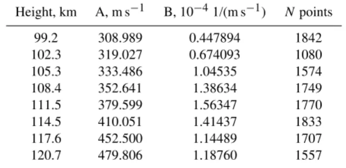
Table 2. ParametersAandBof the fitCS=A+B·VE2
×Bto the
EISCAT data at various heights.
Height, km A, m s−1 B, 10−41/(m s−1) Npoints
99.2 308.989 0.447894 1842
102.3 319.027 0.674093 1080
105.3 333.486 1.04535 1574
108.4 352.641 1.38634 1749
111.5 379.599 1.56347 1770
114.5 410.051 1.41437 1833
117.6 452.500 1.14489 1707
120.7 479.806 1.18760 1557
To quantitatively improve the comparisons with the isothermal ion acoustic speed, we have revisited the depen-denceCS(VE×B)by selecting a data set made of 5 EISCAT days of observations (Table 1), totaling about 160 h of EIS-CAT CP1 measurements. For these periods, data on temper-ature and electric field were good in terms of quality (consis-tently low error in measurements), while a significant span of electric field magnitudes was achieved. The data were ob-tained with a height resolution of∼3 km and an integration time of 2 min.
The isothermalCSvalues were computed for every height
from the measured electron and ion temperatures (TeandTi).
Points with error in temperature measurements of >200 K were rejected. The scatter plot ofCSversusVE×Bwas then fit with a quadratic dependence of a typeCS=A+B·VE2×B.
The inferred coefficients A andB were found for the en-tire data set and then for individual UT hours. Since only minor variations of the coefficients were found for various hours, we report here coefficients for the entire data set (Ta-ble 2). One should note here that although the data set under consideration was significant, the data coverage for VE×B>1000 m s−1 was somewhat limited, and very few points were obtained forVE×Bin excess of 1500 m s−1.
Figure 1 gives a graphical presentation of the inferred de-pendencies for all heights. One can see a general increase of CS withVE×B. The effect is certainly stronger in the mid-dle of the electrojet, with the fastest rate of increase with VE×B at 111 km. This is consistent with previous reports that turbulent electron heating is strongest at these heights (e.g., St.-Maurice et al., 1990). It is however of interest to note that the Nielsen and Schlegel (1985) curve (blue dashed line in Fig. 1) has a similar shape but that it is offset by some∼100 m s−1(and more asV
E×Bis increased) from the data at 111 km, the center of the elecrojet layer. Nonethe-less, we find that the often quoted nominal 400 m s−1value
Fig. 1. Variation of the isothermal ion-acoustic speed withE×
B magnitude at various heights in the ionosphere (99–121 km)
as inferred from EISCAT measurements between ∼12:00 and
18:00 MLT. Dashed line is the dependence of the VHF radar
ve-locity upon theE×Bmagnitude reported by Nielsen and Schlegel
(1985). Red curve at 111 km corresponds to the height with
strongest variation.
3 HF radar data selection
To investigate the relationship between the HF velocity, E×Bplasma drift andCS, we consider data collected by the
Stokkseyri SuperDARN radar. Figure 2 shows the Stokkseyri radar field of view (FoV), and one can see that the low num-bered beams (0–2) are oriented close to the L-shell direction, the predominant direction of the plasma flow (E×B direc-tion) in the afternoon/evening sector. Computations show that smallest L-shell angles are ∼15◦ at very short range
gates of 3–5; they decrease with range so that the flow an-gle is around zero at the radar range gates of ∼35. At these ranges, F-region echoes are usually observed. Figure 2 also shows the lines of zero off-orthogonality angles for the radar rays at the height of 110 km (for the radar frequency of 12 MHz, the irregularity wavelength of 12.5 m). For density of 3.5×104cm−3, the perfect aspect condition is expected
at range gate 15, while for density of 10×104cm−3it is at
range gate 7. For the above aspect angle estimates, simple Snell’s law was applied to a spherically uniform ionosphere. In this study, we identified a number of events with stable and long-lived concurrent short-range (<630 km, gates 3–10, presumably E-region) and far-range (>700 km but less than ∼2000 km, gates 11–40, F-region) HF echo bands, observed in the afternoon sector. The original idea for this approach
Fig. 2. The field-of-view of the Stokkseyri SuperDARN radar be-tween gates 0 and 24 (ranges 180–1260 km). The height of 110 km is assumed. The blue lines are the zero aspect angle lines for obser-vations under various electron densities in the ionosphere (densities
are also shown in blue in units of 1010m−3)at 110 km and the radar
frequency of 12 MHz. The thick lines are the AACGM magnetic
latitudes of 65◦–75◦.
was given by Milan and Lester (1998). In addition to band stability, we wanted the far-range echoes in the standard Su-perDARN range-time plots to have a high velocity of the or-der of 1000 m s−1or more and echoes at short ranges to have
J. D. Gorin et al.: Velocity of E-region HF echoes under strongly-driven electrojet conditions 239
Fig. 3. Stokkseyri radar velocity-range-gate-time plots for three typical events considered in this study. All data are for beam 1. Notice that the color scales are not all the same.
larger velocity (green color saturates) and constitute a sep-arate band visible in the backscatter power. Figure 3b, for 19 November 2001, illustrates a case of very low velocities persisting for a long period of time. Contrary to the data in Fig. 3a, temporal variations in the F-region velocities do not have any corresponding response in the velocity of the short-range E-region echoes. Figure 3c gives an example of a third type of events: for the period between 20:00 and 20:20 UT on 15 January 2002, velocities at small and large radar range gates are comparable.
4 Velocity comparison in one direction and low-numbered beams
As a first step, we simply compare the Stokkseyri velocity data in beam 1 at short and far ranges. This beam is ori-ented only 15◦–25◦off the L-shell directions (Gorin, 2008).
We consider these differences to be small enough that the comparison would refer at least roughly to theE×B drift direction.
To explain the procedure for the velocity comparison, we present in Fig. 4 the Stokkseyri data (1 November 2001) for the echo power, spectral width and velocity for range gates 0– 40. The data cover half an hour of measurements between 16:00 and 16:30 UT. This has been done for the purpose of illustration only; similar profiles have been considered for each beam and for every radar scan. The red curve in Fig. 4 traces the median value of the respective parameter for each
Fig. 4. Echo power, spectral width and velocity recorded by the Stokkseyri radar in the event of 1 November 2001 in range gates 0– 40. Red curves represent the median value of a respective parameter at various range gates.
gate. One can see that the strongest echoes, at 30–40 dB, were received in range gates 6–8 and that the echo power was gradually decreasing with range gate beyond that. Start-ing from range gate∼18, the power started to increase again, reaching its second maximum (in the range profile) at range gate 21, Fig. 4a. Figure 4b shows that strongest echoes were also the broadest, 200–300 m s−1at the near range gates
ver-sus 100–200 m s−1at the far range gates. The echo velocity,
Fig. 4c, clearly demonstrates that while the velocity at the far range gates was in excess of∼1200 m s−1, at the small
range gates it was only 200–500 m s−1. The velocities in
range gates 15–25 were, in some places, low while at the other places they were high. This is an indication that in these range gates, the echoes were coming from the E-region at one time and from the F-region (above the electrojet layer) at another. It means that the red curve does not characterize typical F-region velocity in these range gates. One can also notice near-zero velocities in large gates; these are likely to be due to some small contribution from ground scatter sig-nals that were not properly filtered out by the algorithm.
Fig. 5.Temporal variations of(a)the echo power,(b)spectral width
and(c)velocity for the E-region and F-region echoes (inferred from
short- and far-range data, as discussed in the text). Red crosses represent the E-region parameters while blue diamonds connected by the blue lines represent F-region parameters.
component along the beam) was inferred as the median value of the velocity set. In this way, data contamination from the E-region and ground scatter echoes was prevented while a significant amount of points were still included into assess-ment. We note that the criteria for echo acceptance (both for the E- and F-region echoes) were that the echo power be larger than 3 dB, the error in the line-of-sight velocity deter-mination be less than 300 m s−1and the echo spectral width
be less than 800 m s−1. These are not very stringent
condi-tions, but they eliminate really poor measurements.
The handling of the E-region data was more complicated. We demonstrated that the observed echo power varies with range (Fig. 4a). This is expected (e.g., Makarevitch et al., 2002b), because the E-region echoes are highly aspect sen-sitive. For the 1 November 2001 event, range gates 6–8 cor-respond to a condition with maximum power and minimum, perhaps zero, aspect angle observations. The velocity of the E-region echoes also shows a maximum in range gates 6–8 though not as obvious as in the echo power. We relate the existence of this maximum to the velocity aspect angle atten-uation at ranges away from the maximum for the echo power; this effect has been demonstrated for both VHF and HF co-herent echoes (e.g., Ogawa et al., 1980; Kustov et al., 1994; Makarevitch et al., 2002b, 2007). To obtain an estimate of the E-region velocity least affected by the aspect angle effect, we considered the mean velocity in three radar cells (among those observed in gates 3–10) corresponding to the ranges
with the maximum echo power at short ranges. More specifi-cally, we would find the range with the maximum echo power in a selected beam, and then average its velocity with the ve-locities found in adjacent range gates. We also estimated the average echo power and spectral width in the selected range gates at each time interval.
Figure 5 presents a time series plot of the average (a) echo power, (b) spectral width and (c) velocity for the event of 1 November 2001. The E-region echoes are stronger and broader than the F-region echoes (Fig. 5a and b) and the E-region velocity magnitudes are near the ion-acoustic speed while the F-region velocity (electron drift component along the beam) is very large (∼1300 m s−1) and varies more
sig-nificantly. We estimated the velocity ratio in the E- and F-regions,R=VE/VFand found thatRholds steady at a value
around 0.3.
A number of events was processed in the same way with the goal to assess the velocities of E-region echoes in relation to theE×Bdrift magnitude (that we associate with the ve-locities of the F-region echoes) and toCS. The isothermalCS
estimates were obtained using the empirical quadratic formu-las discussed in Sect. 2. We present the results of this analysis in Fig. 6. In Fig. 6a we show data for the three events already presented in Fig. 3. For 1 November 2001 (red diamonds), the cloud of points is spread around the line described byCS
at 99 km. For 15 January 2002 (blue points), one can dis-tinguish 2 types of behavior. One cluster is aligned with the dashed (pink) line of ideal coincidence of the E-region ve-locity and theE×Bdrift. Quite a few points, however, are shifted from the dashed line and cover a wide range of pos-sibleCS values. For 19 November 2001 (green points), the
velocities are significantly smaller than both theE×B and CSvalues. In this sense, they are similar to what is known to
take place for SuperDARN echoes at large flow angles (e.g., Koustov et al., 2002; Makarevitch et al., 2002a, 2004). These echoes are therefore probably of a different origin. For ex-ample, they often co-exist with low-velocity echoes of op-posite polarity (blue color in Fig. 3c), the so-called HAIR echoes (Milan et al., 2004). The HAIR echoes are believed to be received at large aspect angles and thus involve differ-ent physics. Since the very low-velocity echoes could be of different origin, we decided not to include this kind of events into our statistics.
To enlarge the data set, more events have been processed for observations taken in 1999–2002. Figure 6b gives binned values of the observed E-region velocities for 33 events that all seem to have characteristics similar to the 1 November and 15 January 2001 events. The data spread, indicated by the standard deviation in each bin, is still significant but the trends are obvious: (1) all the points are clustered around the CS line at 99 km and (2) the Doppler velocity generally
J. D. Gorin et al.: Velocity of E-region HF echoes under strongly-driven electrojet conditions 241
Fig. 6. (a)Scatter plot of the Stokkseyri E-region velocity in beams 1 and 2 versusE×Bdrift magnitude (estimated from F-region velocity data, as discussed in the text) for the events of 1 November 2001 (red), 19 November 2001 (green) and 15 January 2002 (blue). These are
three typical types of events identified in the data. Shown also are curves for the dependenceCS(E×B)at the heights of 99, 108 and 121 km,
reported in Fig. 1. Dashed and pink line is an ideal coincidence line.(b)Binned values of the Stokkseyri velocity in beams 1 and 2 (black
dots) with standard deviation in each bin (vertical bars) and the number of values involved in averaging over each bin. The curved lines are
the same as in panel(a).
5 Observations in all beams
The above analysis can be criticized in 3 ways. First, the flow angles are slightly different at the far and short ranges of the Stokkseyri FoV. Secondly, the direction of theE×B drift can differ from the assumed direction, as the flow might not be perfectly aligned with an L-shell. Finally, the peak velocities of the E-region echoes might not themselves be aligned with the E×B direction. We now address these points using data collected from all the beams as opposed to just those beams that are closely aligned with the L-shells. Such an investigation has its own merit, as the characteris-tic dependence of E-region echoes on the flow angle is not well established (e.g., Milan and Lester, 1998, 2001). In this section, we use the L-shell angleφas the reference for the flow angle directions, which themselves will be described by the flow angleθ. The angle φ will be measured counter-clockwise from the line of constant magnetic latitude to the Stokkseyri line-of-sight direction. Every range gate within the Stokkseyri FoV then has its own unique L-shell angle.
5.1 Flow angle variation for velocity
We first consider individual velocity measurements for the entire event of 1 November 2001 for both the E-region and F-region echoes in Fig. 7. Here all the data are plotted using scatter plots. The data points have been binned according to the L-shell angleφ. Clearly, the velocity of the F-region echoes changes drastically from∼1400 m s−1atφ
=20◦to
∼0 m s−1atφ
=70◦. Note that the data set is somewhat
af-fected by mixed/ground scatter echoes at larger values ofφ. Figure 7 also shows the cosine fits to the binned values of the velocity (dashed lines). Looking at how the points are located around the fitted cosine lines, one can conclude that selection of this functional dependence is reasonable for both the E- and F-region echoes. This is one of the arguments for using cosine functions below to fit the binned data.
There are significant differences between the maximum F-and E-region velocities in the cosine fits, namely, 1330 m s−1
versus 393 m s−1, respectively (a velocity ratio of
∼0.3). This result fully agrees with the results from the low-numbered beam analysis presented in Sect. 4. Another in-teresting feature is that the velocity maxima in the E- and F-regions are achieved at slightly different φ angles (−7◦
versus+18◦, respectively, we show the mutual orientation
of the E-region and F-region velocity peaks on the insert). This feature is investigated further in Sect. 5.4. Note that a similar analysis of many other events showed similar results. The variations shown in Fig. 7 are, in other words, typical.
5.2 Approach to analysis of individual scan data
F region
E region
Stokkseyri: 01 Nov 2001, 15:20-18:00 UT
-1330*cos( +18.2 )f 0
-393*cos( -7.4 )f 0
0 20 40 60 80 L-Shell Angle , degf
0 -2
-4
-6 -8 0 -5 -10
-15 20
V
elocity
, 100 m/s
V
elocity
, 100 m/s
E
ExB E region velocity
Fig. 7.Scatter plot of the Stokkseyri F- and E-region velocities for all scans between 15:20 and 18:00 UT on 1 November 2001. Dia-monds with vertical bars are binned values of the velocity and the standard deviation for each bin. Red dashed lines represent the co-sine fits to the binned velocity values. Inferred parameters of the fits are shown in the right bottom corner of each panel. Inset be-tween the panels explains inferred mutual orientation of the E- and
F-region velocity (E×Bdrift) with respect to the L-shell direction
(dashed line).
Figure 8b presents the velocity data in a more readable form. Here, red crosses show the velocity within the as-sumed E-region ranges (gates 3–10) and diamonds show the velocities within the assumed F-region ranges (gates>11– 40). Two sets of points are recognizable here: one set, di-amonds, is stretching to high velocities up to∼1600 m s−1
and the other one is a cloud of points located near velocities of 300–500 m s−1. Within the second cluster, there are a few
points that are classified as F-region scatter; as stated earlier, these were received in gates 11–15. These are likely E-region echoes still, with the fact that they belong to the cloud of E-region points in Fig. 8b supporting this assumption.
To characterize the E- and F-region sets, we fitted the ve-locities with a cosine function of the formV =V0·cos(φ− φ0), where the coefficientV0represents the peak line-of-sight
velocity andφ0 is the L-shell angle of that velocity
maxi-mum. The major problem in accomplishing this task is that there is a significant scatter in the data, especially in the low-velocity band. Another problem is the overlap of velocities mentioned above: at small angles, some far-range veloci-ties fall into the second group, and are associated with E-region echoes. In addition, there is an overlap between the two data sets at angles of 60◦–70◦. To overcome these
dif-ficulties, two different procedures were attempted. With the first procedure, it was decided to apply a cosine fit straight to velocity versus L-shell angle scatter plots of the type
pre-sented in Fig. 8b; in this instance, this resulted in dependen-ciesVF= −1630·cos(φ+18◦)andVE= −390·cos(φ−4◦)
for the F- and E-region echoes, respectively, after neglecting F-region velocities greater than−500 m s−1and L-shell
an-gles less than 40◦. However, it turned out that the number of
scans comparable in quality to the one shown in Fig. 8a, b was low for this event, and the situation was worse for other events in the database. For these reasons, it was decided to do a preliminary averaging of the data before performing the cosine fit. That is to say: at first, data in each beam posi-tion were considered separately, and the velocity estimates for the E- and F-region echoes were done as described in Sect. 4. Specifically, for the E-region, we found the range with the maximum echo power in the selected beam, and then averaged this velocity with the velocity in the adjacent range gates. This velocity was assigned to the L-shell angle of the range gate of the power maximum. For the F-region echoes, the velocity maximum was found along the beam in range gates 11–40 and then this value was averaged over all other observed velocities whose magnitude was within 40 % of the peak within that beam. This velocity was assigned to the L-shell angle of the range gate of the velocity maximum. Figure 8c and d illustrates what emerged from this approach with dependencies given byVF= −1560·cos(φ+10◦)and VE= −480·cos(φ+0◦)for the F- and E-region echoes
re-spectively. Although the obtained parameters of the cosine function differ from the first approach, we believe that the differences are not significant, and that this justified using the second approach for the bulk of the data set. In fact, the fits performed in the second way produced a closer visual agreement with the cloud of points than the first method of simply fitting to the clouds of points first. The reason is that even a couple of outliers from the general trend affect the fit significantly while these outliers are removed in the second approach.
The cosine function fit to the velocity data was done by us-ing a Levenberg-Marquardt algorithm (Press and Vetterlus-ing, 1986), which provides a numerical solution to the problem of minimizing a non-linear function over the space of its param-eters, in this case the peak velocity,V0, and the phase shift, φ0. Based on several trial-and-error work, it was determined
that the fitted result should be discarded if the standard error between the fitted cosine curve and the peak line-of-sight ve-locity estimates was greater than 300 m s−1for the F-region
fits and greater than 150 m s−1for the E-region fits.
5.3 E-region velocity maximum andE×Bmagnitude
J. D. Gorin et al.: Velocity of E-region HF echoes under strongly-driven electrojet conditions 243
Fig. 8. (a)Stokkseyri HF radar velocity map obtained on 1 November 2001 at 15:58:00–15:59:48 UT. The magnetic parallels of 70◦and 80◦
are shown by grey line to simplify estimates of the L-shell angleφ.(b)Scatter plot of the velocity versus L-shell angle for the map shown
in panel(a)and cosine fit results for the fit to Stokkseyri velocities for 1 November 2001 at 15:58–16:00 UT.(c)Cosine fit results for the
fit to the peak line-of-sight F-region velocity estimates for 1 November 2001 at 15:58–16:00 UT.(d)Cosine fit results for the fit to the peak
line-of-sight E-region velocity estimates for 1 November 2001 at 15:58–16:00 UT.
in Sect. 5.2. For other Stokkseyri scans, the task was not as straightforward, as the data scatter was sometimes consider-able. The decision was made to consider only those scans for which the fit with the cosine function was perceived to be reasonable. With respect to the F-region data, the violation of this assumption meant that the electric field distribution within the radar FoV was simply not uniform. With respect to the E-region echoes, our adoption of the cosine depen-dence at small flow angles can be justified by the results of Bahcivan et al. (2005) at 30 MHz, particularly after bearing in mind that at large flow angles a cosine fit is the traditional way to describe the data (e.g., Villain et al., 1987; Uspen-sky et al., 2001; Makarevitch et al., 2002b). We also showed in Fig. 7 that the scatter plots of the velocity versus L-shell angle for the entire interval can be well represented by the cosine function.
We ended up with a selection of a small number of Stokkseyri scans that had reasonable (according to the crite-ria specified above) data for fitting both the E- and F-region velocities and we found the maximum E-region velocity and the direction of this maximum. Data for four of these events are presented here: 1 November 2001, 17 November 2001, 15 January 2002 and 3 March 2002. For these days, reason-able amount of good scans was found so that total of 186 data points was available.
Figure 9 presents the values of the E-region velocities that we obtained, binned in terms of theE×B drift magnitude determined from F-region data. Vertical bars indicate the standard deviation for each bin. We also show the lines CS(VE×B)inferred from EISCAT data at three heights (see Sect. 2). Although the number of points is limited and their scatter is significant, one reliable conclusion emerges: the HF velocity is near theCS values at 99 km. In other words, the
data that we retrieved from Stokkseyri do not contradict the Bahcivan et al. (2005) hypothesis, but only if one assumes that the HF echoes are consistently coming from the bottom of the electrojet layer.
The data presented in Fig. 9 do not show a general ten-dency of the velocity increase withE×Bdrift, contrary to the data of Fig. 6. We attribute this to a relatively small num-ber of good scans that we were able to identify in this ap-proach, poorer coverage of smallest and largest drift magni-tudes, and significant data spread. The binned values of the velocity themselves are, however, in reasonable agreement with those in Fig. 6.
5.4 Direction of the E-region velocity maximum and the E×Bdirection
Fig. 9. Maximum E-region velocity (derived from the Stokkseyri
scan data and fitting procedure) for variousE×Bdrift magnitudes.
Successful fittings for four events were considered: 1 Novem-ber 2001, 17 NovemNovem-ber 2001, 15 January 2002 and 3 March 2002.
Solid lines are the dependenceCS(E×B)at the heights of 99, 108
and 121 km, reported in Fig. 1.
the points in the event (an hour or longer duration) are con-sidered. To assess this effect for individual scans, we now examine the results of the cosine fitting for 186 Stokkseyri scans considered in Sect. 5.3. Figure 10a gives a histogram distribution of the differences between the azimuths of the F-and E-region maximum velocity. The bell shaped diagram suggests that there is a statistical mean value of the shift of 22◦–24◦, with the F-region (E-region) echoes having small
positive (negative) azimuth. This implies that the E-region velocity maximum is generally shifted by∼20◦towards the
direction of the electric field, just like shown in the insert of Fig. 7 (the scans were in the afternoon/evening sector with a northward oriented electric field). We also examined how the above shift changes withE×B magnitude, Fig. 10b. The shift is more pronounced at larger E×B magnitudes; the linear fit to the obtained points gives1φ◦=0.016·VE×B−2 degrees and the trend of the data (shown in red, Fig. 10b) agrees with the fitted result.
6 Discussion
Concurrent measurements of theE×B drift and E-region HF echo velocity are very limited, especially for observa-tions roughly along the drift direction. Davies et al. (1999) and Koustov et al. (2005) involved EISCAT and DMSP data for HF velocity studies. They found smaller E-region ve-locities as compared to the l-o-s component of theE×B
Fig. 10. (a)Occurrence histogram for the difference in the azimuth
between the direction of theE×Bdrift magnitude and the E-region
velocity maximum (1φ). Maximum of the Gaussian fit to the
his-togram occurs at−16.3◦.(b)Scatter plot of1φversus theE×B
drift magnitude. Solid dots with bars represent binned values and standard deviations within each bin. Also shown are a linear fit line and its parameters.
drift, but the flow angles of measurements were not reported and no comparison with the expected CS values were
per-formed. A re-assessment of the published plots shows that quite a few points had velocities below the nominalCSvalue
of 400 m s−1.
Several papers have discussed the properties of E-region HF echoes with near-CS velocities (so-called “type 1”
echoes), referring to a nominal value ofCS=400 m s−1(e.g.,
Villain et al., 1987, 1990; Hanuise et al., 1991; Milan and Lester, 1998, 2001). In the current study we addressed the issue further by estimatingCSvalues using a statistical
rela-tionship betweenE×BandCSinferred from EISCAT
J. D. Gorin et al.: Velocity of E-region HF echoes under strongly-driven electrojet conditions 245
Two approaches were employed: (1) a straight comparison of the velocities at short (E-region) and far (F-region) radar ranges and (2) fitting the velocity data in all beams with the cosine function and inferring maximum velocity for the E-and F-region echoes. Both approaches lead us to a conclu-sion that the typical velocities of HF E-region echoes for ob-servations close to theE×Bdirection are comparable to the expectedCSvalues. The observations also show a tendency
to increase withE×B but the magnitude of the velocities corresponds to ion acoustic-speeds that would have to come predominantly from the bottom of the electrojet,<100 km. 6.1 Magnitude of saturation speed
The results obtained here disagree with several previous studies. For example, Milan and Lester (2001) reported Pykkvibaer HF velocities to be statistically larger than the nominalCSvalue. They did identify a cluster of points with
velocities close to it (perhaps, the “genuine” type 1 echoes), but overall, it seems that velocities above the nominal CS
dominated their datasets. E-region velocities greater than 400 m s−1 have also been reported by Hanuise et al. (1991)
who explained them by invoking echo reception from rela-tively large heights. Uspensky et al. (2001) reported E-region velocities of up to 700 m s−1. Makarevitch et al. (2002a)
presented HF data with velocities up to 700 m s−1that were
larger that concurrently detected VHF (50 MHz) velocities. At 30 MHz, Bahcivan et al. (2005) showed echo velocities up to 600 m s−1that were believed to be close toC
S.
Makare-vich (2008, 2010) also expanded original findings by Mi-lan and Lester (2001) and investigated SuperDARN E-region echoes with velocities well above the nominalCSvalue. Our
analysis indicates that although high E-region HF velocities of up 600–700 m s−1 can be detected, these correspond to
strong electric fields and very highCS values. For example,
no binned HF velocity in our analysis exceeded 500 m s−1
and in fact the trends at 99 km were only extended up to just below 500 m s−1at 2000 m s−1(Figs. 6b and 9). Statistically
speaking, the velocities observed in the current study were below what one expects for theCS values in the middle of
the electrojet layer.
The reasons for the observation of lower-than-expected HF velocities in our case are not entirely clear. One factor may be that the electric field was, in reality, somewhat smaller than inferred from the far-range velocity data; some decrease of its magnitude towards lower latitudes is highly expected. Retroactively, after the performed analysis, we attempted to isolate Stokkseyri events with velocities aboveCS, by a
sim-ple visual search through the Stokkseyri data base. We were not able to find too many events when the short-range veloc-ity was clearly close to the velocveloc-ity at far ranges.
It has also become clear over the years that several factors need to be considered before assessing what the speed of E-region irregularities should be for directions comparable to theE×Bdirection. To start with and, as mentioned earlier,
with due exceptions, repeated observations strongly suggest that the phase speed of E-region structures at their maximum amplitude is very often comparable to the threshold speed, namely, the isothermal ion-acoustic speed (e.g., Sahr and Fe-jer, 1996). A basic explanation for this has been advanced by Liperovski et al. (1999) and St.-Maurice and Hamza (2001) who both argued that, in effect, as the amplitude of a sub-structure grows, the electric field inside it must rotate and decrease in magnitude until the growth rate becomes zero, at which point the structure moves at the threshold speed while having reached its maximum amplitude. Numeri-cal simulations also strongly suggest that the largest am-plitude structures should move at a speed somewhat larger than the threshold speed of the instability while the electric field clearly rotates inside them (e.g., Otani and Oppenheim, 1998; Oppenheim et al., 2008). Many factors conspire to the production of threshold speeds that, however, differ from the isothermal ion-acoustic speed. For one thing, the elec-trons are neither isothermal nor isotropic (e.g., Dimant and Sudan, 1995, 1997; Kagan and St.-Maurice, 2004; Kissack et al., 2008). At decameter wavelengths, this conspires to in-crease the threshold speed of the irregularities, particularly at the lower altitudes (e.g., Kagan and St.-Maurice, 2004). However, increasing the aspect angle from 0 to 1 degree un-der these conditions means that the net increase above the isothermal ion-acoustic speed should only be of the order of 10 percent (Kagan and St.-Maurice, 2004). At the equator, when the aspect angle is sometimes very small, the increase at the lower altitude is, however, sometimes of the order of 30 percent, which has been observed, complete with an increase of the phase velocity with decreasing altitude during strong electric field conditions (e.g., St.-Maurice et al., 2003).
Two other factors are known to modify the speed of ir-regularities at saturation: turbulence, and density gradients. The more strongly turbulent the plasma is, the broader the spectrum becomes and the slower the observed phase veloc-ity becomes compared to the threshold speed (Hamza and St.-Maurice, 1993). The fact that, even along L-shells, the E-region spectra in our data set are quite wide (of the or-der of 300 m s−1in Doppler units) might therefore be
signifi-cant. Finally, if they favor growth, ambient density gradients can, particularly at decameter wavelengths, easily decrease the threshold speed and vice-versa for unfavorable gradient directions (Hanuise et al., 1991; St.-Maurice et al., 1994). In addition to physical constraints, one should also keep in mind that the Doppler shift of HF radar echoes is affected by the index of refraction of the medium (Ponomarenko et al., 2009). The effect can be as large as a 20 to 30 percent un-derestimation of the true drift and is strongest for the larger ambient plasma densities (Gillies et al., 2009).
Observationally, all our cases were for relatively large E-region electron density (>105cm−3) since only for these
-800 -600 -400 -200 0 Velocity, m/s
0 20 40 60 80
L-Shell Angle ,
f
, deg
01/11/2001 15:58-16:00 UT
315-630 km
Fig. 11. Scatter plot of the E-region velocity (red crosses) versus L-shell angle for the Stokkseyri scan 15:58:00–15:59:48 UT (the same as in Fig. 8b), cosine fit line for these data (dashed line), and expected velocity variations with L-shell angle according to Bah-civan et al. (2005) (dash-dotted line) and empirical dependence by Nielsen et al. (2002) for VHF (dotted line).
be that only the bottom part of the potential echo-detection curve is effective (for the curve, see Uspensky et al., 1994, and Uspensky et al., 2001). Generally, such an assumption is difficult to justify. Information on elevation angles would help testing this possibility, but elevation angles are not reli-able for the Stokkseyri radar.
Having taken all the above factors into consideration, we conclude that the need to have E-region echoes at close prox-imity in order to have small enough angle conditions is the most important factor for observed threshold speeds that are lower than in other observations. The reason is that in order to obtain echoes at close proximity, the E-region density it-self has to be large. This means in turn that the Doppler shift correction due to the index of refraction is on the high side, perhaps leading to apparent speeds that are as large as 30 % smaller than the real speeds. In addition, the aspect angles are probably be on the high side of E-region delectability as well. This means that the threshold speed may well be only 10 % larger than the isothermal ion-acoustic speed even at the lower altitudes. There might be a link between the obser-vation being limited to lower altitudes and the larger spectral widths that we observe (faster decay rates), contributing to a further decrease in the observed threshold speeds.
6.2 Flow angle variation
The other issue addressed by our analysis is the velocity vari-ation with the flow angle. We considered very strong electric field cases so that the FB linear instability cone was fairly wide. We identified a number of events for which the veloc-ity variations in both E- and F-region echoes were
character-ized reasonably well by a cosine function. In this sense, we selected, from the beginning, a class of events that were con-sistent with the idea by Bahcivan et al. (2005) that the varia-tion isVE(θ )=CS·cosθ. As was discussed above, we found
the E-region velocity maximum to be smaller thanCSin the
middle of the electrojet layer but the cosine type of variation was fairly clear in the selected individual cases. A similar variation, although not discussed at length, was seen in the small-flow-angle data presented by Uspensky et al. (2001). The latter paper interpreted the SuperDARN Pykkvibaer E-region velocities in terms of highly inhomogeneous, patchy electric field so that genuine Type 1 echoes (with a veloc-ity of 400 m s−1speed) coexisted with high-velocity echoes
(∼700 m s−1) but at quite different azimuths/locations. Since
no F-region velocity estimates were available for the event considered in that study, one cannot judge if their case con-tradicted our results. In the recent studies involving the Su-perDARN radars at Syowa (Makarevich, 2008, 2010) a broad range of flow angles was considered with the E×B esti-mates obtained from farther ranges just as was done in the present work. Although the focus of these studies was on the high-velocity echoes, just like in the present study, the low velocities echoes (<200 m s−1) were also observed
un-der the strongly-driven conditions at small flow angles, with the velocity variation being consistent with a cosine trend. The present study thus provides a critical piece of evidence for the hypothesis that these echoes originate from the bot-tom of the electrojet layer by using theCSestimates
directly-driven by theE×Bdrift velocity data. Moreover, the current study shows this to occur on a statistical basis. An impor-tant difference, however, appears to be that no high-velocity counterparts were observed in the current study.
J. D. Gorin et al.: Velocity of E-region HF echoes under strongly-driven electrojet conditions 247
To illustrate how far the Stokkseyri velocity flow angle variation was from the dependencies reported at VHF we present a typical scan data, Fig. 11, along with expectations of Bahcivan et al. (2005) and Nielsen et al. (2002). In this analysis, we used our estimates ofCSbased on EISCAT data
reported in Sect. 2. At flow angles for which the HF data were available, the velocity is described reasonably well by theCS·cosθdependence. The inferred coefficient of
propor-tionality of∼487 m s−1is smaller than the expected value of CS≈580 m s−1 (dash-dot line atθ=0◦). The relationship
by Nielsen et al. (2002) does not work well; the dotted line is way off the HF data and the cosine-fit curve. One can say that for this scan the Stokkseyri data support the Bahcivan et al. (2005) hypothesis in terms of the flow angle (functional) dependence.
Bahcivan et al. (2005) also proposed that theCS-saturated
FB waves, i.e., propagating exactly with the velocityCS, can
only be observed in a very small flow angle cone and not ev-erywhere within the FB linear instability cone. Stokkseyri observations occasionally do show such a feature for some periods; cases were identified for which the velocity was changing relatively slowly with azimuth at large L-shell an-gles while the velocity was close to the expected values of CS at small L-shell angles, for low-numbered beams. This
feature was also reported by Milan and Lester (2001) for the Pykkvibaer radar. We note, however, that the number of Stokkseyri events with variations of the kind discussed here was low. One possible reason for this is that very low L-shell angles are not available within the Stokkseyri FoV.
6.3 Rotation of the orientation of the maximum velocities
Another interesting result of our all-beam data analysis was existence of a significant average shift between the direction of the E-region velocity maximum and the direction of the E×B drift. Makarevitch et al. (2002a) reported the offset (∼5◦)between the velocity maxima at HF and VHF while
comparing Syowa SuperDARN data and concurrently oper-ated 50-MHz radar data. Earlier, Blix et al. (1996) observed stronger electrostatic fluctuations at the bottom of the E layer away from theE×Bdirection, which is reminiscent of what we observe with the Stokkseyri radar but in terms of the ve-locity. Our data show some weak tendency for the effect to increase with theE×B magnitude. This implies that the shift is harder to detect at averageE×B drifts. The exis-tence of the shift itself has been predicted theoretically in the past using both quasi-linear and nonlinear approaches (e.g., Janhunen, 1994; Sahr and Farley, 1995). The net rotation is also clearly seen in advanced numerical simulations (Oppen-heim et al., 2008) and has been attributed to a linear effect associated with ion heating inside the structures (Oppenheim and Dimant, 2004). However, given its relation to ion heat-ing, this rotation should not be substantial for electric fields smaller than, say, 50 mV m−1, particularly in the bottomside
regions. An alternative would be a result of the rotation in the electric field that routinely has to take place inside the structures. Such a rotation is clearly seen in numerical simu-lations (Otani and Oppenheim, 1998), and its basis has been discussed in terms of the nonlinear effects that must be part of the evolution of the structures (St.-Maurice and Hamza, 2001; Hysell and Drexler, 2006). For areas with an increased electron density, the maximum irregularity velocity would be rotated away from theE×Bdirection towards the electric field direction while areas with depleted electron densities have to rotate in the opposite direction. Further work needs to be done to see if the depletions would contribute less to the total echo signal so that a net rotation in echo power would take place. No matter what, it should be stressed that our finding that the existence of a rotation with respect to the E×Bdirection depends on the magnitude of theE×Bdrift appears to be a new observational result that could put some of the theoretical ideas to the test.
6.4 Other observational features
Our data showed that some Stokkseyri short-range echoes, identified as E-region echoes, may have been from above the electrojet, as their velocities were very close to the ve-locity of far-range F-region echoes. This was seen in one-beam data, Fig. 6, as well in the velocity scan data, Fig. 11, where the velocities of relatively close-range echoes were a better fit with the cluster of F-region velocities rather than E-region velocities. Unfortunately, we are unable to determine whether these echoes were indeed received from above the electrojet heights. It would be interesting to know how often this happens and how often such cases affect the conclusions on the nature of short-range SuperDARN echoes. Simulta-neous observations with incoherent scatter radar would help resolve this issue.
We have not stressed much, but it is worthy to mention that the other characteristics of the considered E-region echoes, the power and spectral width, seem to be quite different from those reported in the past. For example, Hanuise et al. (1991) reported a typical power of∼10 dB (versus ∼30 dB in our cases) and typical width of ∼100 m s1 (versus ∼300 m s−1
in our case) using the Systeme HF d’Etude Radar Polaires et Aurorales (SHERPA) HF radar located at Schefferville, Que-bec. Milan and Lester’s (2001) data are more consistent with what we reported here. We think that the E-region echoes considered in this study are consistent with Type 4 echoes according to the HF echo classification scheme of Milan and Lester (2001). Further studies are required on this aspect of measurements.
One interesting implication of the present work is the fact that we identified a large number of events for which the ve-locity of E-region echoes was much smaller than theE×B electron drift component inferred from concurrent F-region observations. The typical velocity ratio R=VE/VF was
(more data are given by Gorin, 2008). The inferred value R=0.3 for observations along the flow is somewhat smaller than expected since for the FB waves, propagating along the E×B direction, the velocity would be close to the typical ion-acoustic speed of∼500–600 m s−1for enhanced electron
drifts of 1000–1500 m s−1. Our analysis of the data collected
in other beams/directions showed very comparable values for R(∼0.3) which is roughly consistent with earlier conclusion by Makarevitch et al. (2004) who considered the Hankasalmi radar observations at large flow angles. Their typical velocity ratio was∼0.2 for∼4 h period of observations. The current study thus extends the range of flow angle investigated sta-tistically to include small values under the strongly-driven conditions for which the FB instability is definitely opera-tional and derives a representative factor between the E- and F-region velocities.
Because of typically low ratiosR, care must be exercised when SuperDARN convection maps (produced through the approach by Ruohoniemi and Baker, 1998) contain signifi-cant amounts of the E-region data, especially if details of the convection pattern at low latitudes are investigated. This is especially important as the SuperDARN network is rapidly expanding to lower latitudes and the flows equatorward of the auroral oval are the target of upcoming studies so that E-region echoes is very likely to be involved in the analysis.
7 Conclusions
Results from this study can be summarized as follows: 1. By considering EISCAT electron and ion temperature
data and electric field measurements in the CP1 mode, a relationship between the ion-acoustic speed and the magnitude of the E×B drift was established. A quadratic type of dependence was found to reasonably characterize the relationship, similar to the equation for the VHF velocity introduced by Nielsen and Schlegel (1985). Our coefficients of the fits to the EISCAT data are quite different, however, at the expected heights of VHF echoes near the center of the electrojet. Our ve-locities at that height are at least 100 m s−1greater than
in the previous model.
2. The Stokkseyri SuperDARN radar data were used to study relationship between the velocity of short-range HF echoes, theE×Bmagnitude, and the ion-acoustic speed. TheE×B drift estimates have been obtained through the analysis of concurrently detected Stokkseyri F-region echoes at farther ranges under the assumption of a uniform electric field distribution. The maximum E-region velocities were found, statistically speaking, to be smaller than the expected values ofCSin the
mid-dle of the electrojet layer but were consistent with the values ofCS expected for a height of∼99 km. The
ve-locities tended to increase withE×B, similar to the dependenceCS(VE×B)at the height of 99 km.
3. For a large number of individual scans, the Stokkseyri velocity variation with the flow angle was found to be well described by a cosine function. For these cases, the maximum velocity of E-region echoes was seen off theE×Bdirection, with a shift towards the (northward oriented) electric field direction. The mean value of the shift was∼20◦, and the shift increased with the
magni-tude ofE×B.
4. The occurrence of E-region echoes with velocity three and more times smaller than the E×B electron drift strongly suggests that great caution should be exercised before using any E-region data to derive SuperDARN convection maps, as it could lead to serious underesti-mations of the electric field.
Acknowledgements. This work was supported by an NSERC
(Canada) grant to AVK. A longtime care of the Stokkseyri radar operation by late J.-P. Villain is appreciated. Without his tireless ef-forts this study would have not been possible. We are indebted to the director and staff of EISCAT for operating the facility and supply-ing the data. EISCAT is an international association supported by research organizations in China (CRIRP), Finland (SA), Germany (DFG), Japan (NIPR and STEL), Norway (NFR), Sweden (VR), and the United Kingdom (PPARC). The authors thank R. Fiori for the help in analysis of EISCAT temperature data.
Topical Editor K. Kauristie thanks Y. Dimant and another anonymous referee for their help in evaluating this paper.
References
Bahcivan, H.: Plasma wave heating during extreme electric fields in the high-latitude E region, Geophys. Res. Lett., 34, L15106, doi:10.1029/2006GL029236, 2007.
Bahcivan, H. and Hysell, D. L.: A model of secondary Farley-Buneman waves in the auroral electrojet, J. Geophys. Res., 111, A01304, doi:10.1029/2005JA011408, 2006.
Bahcivan, H., Hysell, D. L., Larsen, M. F., and Pfaff, R. F.: The 30-MHz imaging radar observations of auroral irregularities during the JOULE campaign, J. Geophys. Res., 110, A05307, doi:10.1029/2004JA010975, 2005.
Blix, T. A., Thrane, E. V., Kirkwood, S., Dimant, Y. S., and Sudan, R. N.: Experimental evidence for unstable waves in the lower E/upper D-region excited near the bisector between the electric field and the drift velocity, Geophys. Res. Lett., 23, 2137–2140, 1996.
Chen, P.-R., Yi, L., and Nielsen, E.: Variations of the mean phase velocity of 1-m ionospheric plasma waves with the plasma elec-tron temperature, J. Geophys. Res., 100, 1647–1652, 1995. Chisham, G., Lester, M., Milan, S. E., Freeman, M. P., Bristow, W.
di-J. D. Gorin et al.: Velocity of E-region HF echoes under strongly-driven electrojet conditions 249
rections, Surv. Geophys., 28, 33–109, doi:10.1007/s10712-007-9017-8, 2007.
Davies, J. A., Lester, M., Milan, S. E., and Yeoman, T. K.: A com-parison of velocity measurements from the CUTLASS Finland radar and the EISCAT UHF system, Ann. Geophys., 17, 892– 902, doi:10.1007/s00585-999-0892-9, 1999.
Dimant, Y. S. and Milikh, G. M.: Model of anomalous electron heating in the E region: 1. Basic theory, J. Geophys. Res., 108, 1350, doi:10.1029/2002JA009524, 2003.
Dimant, Y. S. and Sudan, R. N.: Kinetic theory of the Farley- Bune-man instability in the E-region of the ionosphere, J. Geophys. Res., 100, 14605–14623, 1995.
Dimant, Y. S. and Sudan, R. N.: Physical nature of a new cross-field current-driven instability in the lower ionosphere, J. Geophys. Res., 102, 2551–2563, 1997.
Farley, D. T. and Providakes, J.: The variation with Te and Ti of the velocity of unstable ionospheric two-stream waves, J. Geophys. Res., 94, 15415–15420, 1989.
Foster, J. C. and Erickson, P. E.: Simultaneous observations of E-region coherent backscatter and electric field amplitude at F re-gion heights with the Millstone Hill UHF radar, Geophys. Res. Lett., 27, 3177–3180, 2000.
Gillies, R. G., Hussey, G. C., Sofko, G. J., McWilliams, K. A., Fiori, R. A. D., Ponomarenko, P. V., and St.-Maurice, J.-P.: Improve-ment of SuperDARN velocity measureImprove-ments by estimating the index of refraction in the scattering region using interferome-try, J. Geophys. Res., 114, A07305, doi:10.1029/2008JA013967, 2009.
Gorin, J. A.: Velocity of decameter electrojet irregularities at strongly driven conditions, MSc Thesis, U of Saskatchewan, Saskatoon, Canada, 2008.
Haldoupis, C. and Schlegel, K.: Direct comparison of 1-m irregular-ity phase velocirregular-ity and ion-acoustic speeds in the auroral E-region ionosphere, J. Geophys. Res., 95, 18989–19000, 1990.
Hamza, A. M. and St.-Maurice, J.-P.: A turbulent theoretical frame-work for the study of current-driven E region irregularities at high latitudes: Basic derivation and application to gradient-free situa-tions, J. Geophys. Res., 98, 11587–11599, 1993.
Hanuise, C., Villain, J.-P., Cerisier, J. C., Senior, C., Ruohoniemi, J. M., Greenwald, R. A., and Baker, K. B.: Statistical study of high-latitude E-region Doppler spectra obtained with SHERPA HF radar, Ann. Geophys., 9, 273–285, 1991.
Hysell, D. L. and Drexler, J.: Polarization of elliptic E
re-gion plasma irregularities and implications for coherent radar backscatter from Farley-Buneman waves, Radio Sci., 41, RS4015, doi:10.1029/2005RS003424, 2006.
Janhunen, P.: Perpendicular particle simulation of the E region Farley-Buneman instability, J. Geophys. Res., 99, 11461–11473, 1994.
Jones, B., Williams, P. J. S., Schlegel, K., Robinson, T., and Hag-gstrom, I.: Interpretation of enhanced electron temperatures mea-sured in the auroral E-region during the ERRRIS campaign, Ann. Geophys., 9, 55–59, 1991.
Kagan, L. M. and St.-Maurice, J.-P.: Impact of electron thermal effects on Farley-Buneman waves at arbitrary aspect angles, J. Geophys. Res., 109, A12302, doi:10.1029/2004JA010444, 2004. Kissack, R. S., St.-Maurice, J.-P., and Moorcroft, D. R.: Electron thermal effects on the Farley-Buneman fluid dispersion relation, Plasma Phys., 2, 1032–1055, 1995.
Kissack, R. S., Kagan, L. M., and St.-Maurice, J.-P.: Thermal effects on Farley-Buneman waves at nonzero aspect and flow angles. II. Behavior near threshold, Physics of Plasmas, 15-2, 022902-022902-17, 2008.
Kofman, W. and Nielsen, E.: STARE and EISCAT measurements: Evidence for the limitation of STARE Doppler velocity obser-vations by the acoustic velocity, J. Geophys. Res., 95, 131–136, 1990.
Koustov, A. V., Igarashi, K., Andr´e, D., Ohtaka, K., Sato, N., Ya-magishi, H., and Yukimatu, A. S.: Observations of 50- and 12-MHz auroral coherent echoes at the Antarctic Syowa station, J. Geophys. Res., 106, 12875–12887, 2001.
Koustov, A. V., Danskin, D. W., Uspensky, M. V., Ogawa, T., Jan-hunen, P., Nishitani, N., Nozawa, S., Lester, M., and Milan, S.: Velocities of auroral coherent echoes at 12 and 144 MHz, Ann. Geophys., 20, 1647–1661, doi:10.5194/angeo-20-1647-2002, 2002.
Koustov, A. V., Danskin, D. W., Makarevitch, R. A., and Gorin, J. D.: On the relationship between the velocity of E-region HF
echoes andE×Bplasma drift, Ann. Geophys., 23, 371–378,
doi:10.5194/angeo-23-371-2005, 2005.
Kustov, A. V., Uspensky, M. V., Sofko, G. J., Koehler, J. A., and Mu, J.: Aspect angle dependence of the radar aurora Doppler velocity, J. Geophys. Res., 99, 2131–2144, 1994.
Liperovsky, V. A., Meister, C. V., and Kustov, A. V.: Stabilization of the Farley-Buneman instability by three-wave interaction as consequence of the modification of the speed of energy transfer from an external field, Atron. Nachr., 320, 77, 1999.
Makarevich, R. A.: HF radar observations of high-velocity E-region echoes from the eastward auroral electrojet, J. Geophys. Res., 113, A09321, doi:10.1029/2008JA013204, 2008.
Makarevich, R. A.: On the occurrence of high-velocity E-region echoes in SuperDARN observations, J. Geophys. Res., 115, A07302, doi:10.1029/2009JA014698, 2010.
Makarevich, R. A., Koustov, A. V., Senior, A., Uspensky, M., Honary, F., and Dyson, P. L.: Aspect angle dependence of the E region irregularity velocity at large flow angles, J. Geophys. Res., 112, A11303, doi:10.1029/2007JA012342, 2007.
Makarevitch, R. A., Ogawa, T., Igarashi, K., Koustov, A. V., Sato, N., Ohtaka, K., Yamagishi, H., and Yukimatu, A. S.: On the power-velocity relationship for 12- and 50-MHz auroral coherent echoes, J. Geophys. Res., 106, 15455–15469, 2001.
Makarevitch, R. A., Koustov, A. V., Igarashi, K., Sato, N., Ogawa, T., Ohtaka, K., Yamagishi, H., and Yukimatu, A. S.: Comparison of flow angle variations of E-region echo characteristics at VHF and HF, Adv. Polar Upper Atm. Res., 16, 59–83, 2002a. Makarevitch, R. A., Koustov, A. V., Sofko, G., Andr´e, D., and
Ogawa, T.: Multi-frequency measurements of HF Doppler ve-locity in the auroral E region, J. Geophys. Res., 107, 1212, doi:10.1029/2001JA000268, 2002b.
Makarevitch, R. A., Honary, F., and Koustov, A. V.: Simultaneous HF measurements of E- and F-region Doppler velocities at large flow angles, Ann. Geophys., 22, 1177–1185, doi:10.5194/angeo-22-1177-2004, 2004.
Milan, S. E. and Lester, M.: Simultaneous observations at differ-ent altitudes of ionospheric backscatter in the eastward electro-jet, Ann. Geophys., 16, 55–68, doi:10.1007/s00585-997-0055-9, 1998.