SRef-ID: 1432-0576/ag/2004-22-2073 © European Geosciences Union 2004
Annales
Geophysicae
Spacecraft potential effects on electron moments derived from a
perfect plasma detector
V. G´enot1,*and S. J. Schwartz1
1Astronomy Unit, Queen Mary, University of London, Mile End Road, London E1 4NS, England, UK *Now permanently at CESR, Toulouse, France
Received: 16 April 2003 – Revised: 14 January 2004 – Accepted: 28 January 2004 – Published: 14 June 2004
Abstract.A complete computation of the effect of the space-craft potential on electron moments is presented. We adopt the perfect detector concept to estimate how measured den-sity, velocity and temperature are affected by the constraints imposed by the detector, such as the finite lower energy cut-off and the spacecraft potential. We investigate the role of the potential in different plasma regimes usually crossed by satellites. It appears that the solar wind is the region where the moments are most compromised, as the particle temper-ature is low. To a lesser extent the moments calculated in the magnetosheath may also deviate from the real moments, displaying up to 40% overestimation for the density under typical detector operation. The analysis allows us to identify a range of spacecraft potential values which minimizes the variation in the estimation; it is found that it corresponds to the common value adopted by potential controlling experi-ments.
Key words. Space plasma physics (spacecraft sheaths, wakes, charging; experimental and mathematical techniques; instruments and techniques)
1 Introduction
The knowledge of plasma parameters, such as density and temperature, which are moments of the particle distribution functions, is fundamental to any analysis both in space and in the laboratory contexts (see the review in Paschmann et al., 1998). In this aim, the spectrometer technique is based on the direct measurement of particles whose trajectories and energies may be modified by the spacecraft electrical poten-tial. Once the effect of the latter is understood, it is possi-ble to extract accurate density, velocity and temperature from Correspondence to:V. G´enot
the spectrometer measurements. If the full set of spectrom-eter data are available, the moment sums may be performed on the ground after allowing the spacecraft-induced effects. However, limited telemetry often results in limited transmit-ted particle data, and moments are often computransmit-ted onboard. Deducing accurate information from such onboard moments requires techniques such as those we develop in this paper.
Whereas the direct detection of the plasma populations with an energy spectrometer seems the most obvious solu-tion, several other alternative methods have been designed to avoid the spectrometer limitations and constraints. These techniques are based either on electrical or wave measure-ments: the fluctuations in the Langmuir probe collected cur-rent result from fluctuations in the density, the temperature and the floating spacecraft potential (Hilgers et al., 1992); differential potential measurements with double probes pro-vide a diagnostic of the density linking it directly to the spacecraft potential (Laakso et al., 1998); finally, the plasma resonance sounder technique offers an accurate measure of the plasma frequency from which density can be deduced (D´ecr´eau et al., 1997) (further data analysis may also provide the temperature using thermal noise spectroscopy; Meyer-Vernet et al., 1998). The range of validity of these methods, as well as their time resolution, differs, but they all either rely on or are un-affected by the spacecraft potential.
a deficit of negative charge on the spacecraft which will then generally charge positively.
This potential is of course also the cause of uncertainties, as low energy plasma electrons characteristics will be mod-ified as they approach the detector. In this article, we adopt a simple approach to the way the potential affects electrons. It is known as the scalar correction and assumes that the par-ticle trajectories are purely radial to the detector. This is a crude assumption and some authors have developed strate-gies to overcome it (Scime et al., 1994; Bouhram et al., 2002).
However, an analytical approach to the correct modifica-tion of particle trajectories is difficult, even in the case of a 3-D purely spherical detector. Moreover, the spacecraft ge-ometry and fabric also have to be considered if one wants to conduct a detailed study. At this stage an analytical path is no longer the best choice. Global Particle In Cell (PIC) simula-tions may provide the solution as they can take into account geometry and fabric, in addition to computing individual par-ticle trajectories (see, for instance, Singh et al., 2001, in the Polar context). This has also been studied by the SPINE con-sortium with the PicUp3D code (Forest et al., 2001; see also http://spis.onecert.fr/picup3d/index.html).
However, on a much simpler scale, the “perfect” plasma detector may provide estimates of relations between the true moments and those calculated, for example, onboard, with-out compensation for the detector and spacecraft environ-ment. The analytical approach facilitates a survey of the pa-rameter space to analyze the effect on moments. Here we shall investigate the effects of detector energy cutoffs (the lower one is set to avoid the low energy plasma, usually contaminated by photoelectrons), as well as of the space-craft potential. The potential effect is indeed important but has never been tackled before in this context. In Song et al. (1997), the authors correctly state that in the presence of the spacecraft potential the cutoff energies should be eval-uated as the detector’s cutoff energies plus (minus) the po-tential for ions (electrons), but in fact the calculations are done for a null potential and the results are displayed ac-cordingly. In the present paper, we keep the spacecraft po-tential as a variable throughout the calculations. We finally end up with expressions of the measured moments as func-tions of the “real” (free space) moments. The expression are solved analytically and the ratios of measured to “real” mo-ments are displayed as a function of the potential. It is there-fore possible, for given measured plasma conditions, to es-timate the influence of the spacecraft potential. The method resorts to numerical computations only at the last stage; it does, however, require the inversion of a nonlinear integral system. The algorithm proved to be convergent for parame-ters corresponding to nominal operations (solar wind, mag-netosheath and magnetosphere conditions, spacecraft poten-tial up to∼30 V, and lower cutoff∼10 eV). In a degenerate case (considering a non-drifting Maxwellian function for the velocity distribution of electron population, but retaining the potential), Salem et al. (2001), also in the “perfect” detector frame, ingeniously skipped the demanding inversion task by
using a fitting method in restricted density and temperature ranges. This was possible because the measured temperature depended only on the “real” temperature in their case. This method is not applicable for our more general approach.
In the next section we derive the basic equations which link the measured and “real” moments, then in Sect. 3 we briefly discuss the numerical method we developed. In Sect. 4 we present and discuss the results for different typ-ical plasma conditions. Finally, in the conclusion we sum-marize our results, emphasize their limitations and the possi-ble improvements, and we discuss them in the light of more powerful, but more demanding methods.
2 Equations of the moments
In the spacecraft frame the moments of the particle velocity distribution functionfsc are given by the following formula
(vl, vuare the lower and upper speed cutoffs of the detector):
M(ξ )= Z vu
vl
Z π
0
Z 2π
0
v2scdvscsinθscdθscdφscξfsc(vsc, θsc, φsc),(1)
ξ is a parameter which may be a scalar, a vector or a tensor (or higher order) andMis then a moment of order one, two or three, respectively. The physical quantities derived from the measured moments values are the densityN, the velocity vectorV and the pressure tensorP¯given by:
N =M(1) (2)
NV =M(vsc) (3)
¯
P =mM(vscvsc)−mNV V, (4)
wheremis the mass of the particle. Note that some physi-cal quantities of interest (e.g.P¯) involve combinations of the basic momentsM(ξ ).
In the following we shall consider an electron detector; the charge and mass of the electron are−eandme, respectively.
If8sc denotes the spacecraft potential, the conservation of
energy of an electron can be written:
vsc2 =v2−E, (5)
wherevis the velocity in “free space” andEis defined by E= −2e8sc
me
. (6)
It corresponds to the free space energy of an electron which would have zero energy in the spacecraft frame; it is a nega-tive quantity for most of the plasma conditions encountered in space. Along a trajectory in phase space the distribution function remains constant (Liouville theorem):
fsc(vsc, θsc, φsc)=f (v, θ, φ). (7)
be a simple Maxwellian drifting with the velocityV0in the
spacecraft frame and of thermal temperatureT0. Integrating this function over 4πsteradian and over all velocities (which corresponds to an absence of cutoffs, orvl=0 and vu=∞)
gives the total plasma density,N0.f is given by:
f (v, θ, φ)=N0
m
e
2π kT0
3/2
exp
− me
2kT0
(v−V0)2
(8) or
f (v, θ, φ)=N0
m
e
2π kT0
3/2
exp
m
e
2kT0
(−v2−V02+2vV0cosθ )
. (9)
Here we have defined thezdirection to correspond to that of the drift velocityV0. The more general case, for example, in
which the magnetic field defines a second direction associ-ated with an anisotropy in temperature, is considerably more difficult to treat analytically. We now consider that the effect of the spacecraft potential is only effective in the radial direc-tion. This so-called scalar approximation can be expressed byθsc=θ andφsc=φ. Only the velocity magnitude is
af-fected (Eq. 5). We can then rewrite Eq. (1) with respect to the variables(v, θ, φ). The integration elementdvsc has to
be changed according tovscdvsc=vdv. After some algebra,
the measured density, velocity and diagonal elements of the pressure tensor can be expressed by:
N =
m
e
2π kT0
1/2N
0
V0
Z vU
vL
dv
p v2−E
e−
me 2kT0(v−V0)2
−e−
me 2kT0(v+V0)2
(10)
N Vx=N Vy =0 (11)
N Vz=
m
e
2π kT0
1/2N
0
V0
Z vU
vL
dv
(v2−E)
e−
me 2kT0(v−V0)2
+e−
me 2kT0(v+V0)2
−v 2 −E v kT0
meV0
e−
me 2kT0(v−V0)2
−e−
me 2kT0(v+V0)2
(12)
Px=Py=
N0
V02
m
ekT0 2π
1/2Z vU
vL
dv(v
2
−E)32
v
e−
me 2kT0(v−V0)
2
+e−
me 2kT0(v+V0)
2
− kT0
mevV0
e−
me 2kT0(v−V0)2
−e−
me 2kT0(v+V0)2
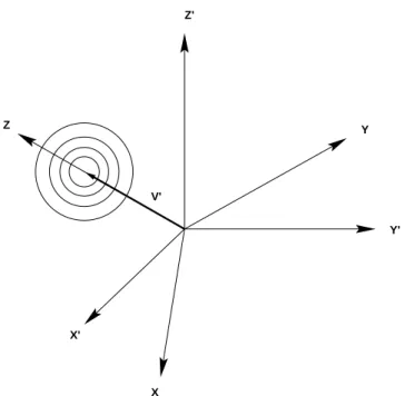
(13) V’ Y’ Y Z’ Z X X’
Fig. 1. Sketch of the measurement (or spacecraft) frame (X′, Y′, Z′)and computation frame (X, Y, Z). The Maxwellian drift velocity isV′.
Pz= −meN Vz2+
N0me
V0
m
e
2π kT0
1/2Z vU
vL
dv
(v2−E)32
e−
me 2kT0(v−V0)2
−e−
me 2kT0(v+V0)2
−m2kT0
evV0
e−
me 2kT0(v−V0)2
+e−
me 2kT0(v+V0)2
+2
kT
0
mevV0
2
e−
me 2kT0(v−V0)2
−e−
me 2kT0(v+V0)2
(14)
withvL,U=
q
v2l,u+E. The expressions calculated by Song et al. (1997) can be recovered forE=0 andvu=∞; those of
Salem et al. (2001) forV0=0 andvu=∞.
LetRbe a rotation which transforms the spacecraft mea-surement frame to a frame where thezaxis is aligned with the measured velocityV′ (see Fig. 1). In the first frame the
mo-ments areN,V′=(V′
x, Vy′, Vz′)andP¯′, whereas in the
sec-ond frame they areN (scalar quantity), V=(0,0,|V′|)and ¯
P. AsRconserves the trace of tensors, the temperatureT
computed fromP¯ or P¯′ is the same: 3N kT=tr(P )¯ =tr(P¯′)
(tr stands for the trace of the tensor). In the following we shall express the diagonal elements of the pressure tensor in the second frame, and then compute the temperature T, frame independent. In practice we do not need to know the details ofR: from the measured velocityV′, we directly
de-duceV which is used in the computation. Since the direction
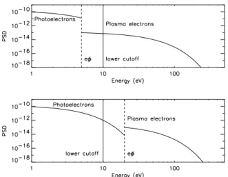
Fig. 2. Electron and photoelectrons distributions for a spacecraft potential smaller than the lower cutoff (upper panel), and for the re-verse situation (bottom panel). The portion of the distribution mea-sured by the detector lies to the right of the solid vertical line.
resulting “real” velocityV0 can then be expressed back in
the original frame asV0V′/V. This transformation enabled us to perform the integration over anglesθ andφ analyti-cally. The remaining integrations over the speedvpresented in Eqs. (10)–(14) require a computational approach.
From the definition of vL, we see that the situation
√
−E>vl, i.e. when the spacecraft potential reaches values higher than the low energy cutoff, is undefined. Actually, in this case we set vL=0 for the computation. In the
ve-locity range[vl,√−E], the detector would measure
photo-electrons, or more generally secondary photo-electrons, which are emitted by the spacecraft (see Fig. 2). These particles re-turn to the detector as their energy is usually less than|E|. Therefore, we could fill the range[vl,
√
−E]with a model of secondary electron distributions. A popular one considers the superposition of two Maxwellians with thermal energies
∼2 eV and∼7 eV (see Grard, 1973, for instance). However, this procedure would add more parameters to our computa-tion and we prefer to restrain our study to the cases√−E<vl. Formev2l/2=10 eV, this corresponds to usual solar wind and
magnetosheath conditions. Nevertheless, we present a re-strictive method (assuming no secondary electrons) for the case√−E>vlwhich then also applies to common magneto-spheric conditions.
3 Numerical method
The interest of the above analysis is to cast estimations based on measured moments to an almost fully analytical form. However, integrations over speeds cannot be determined ana-lytically. The cutoffs are fixed by the particle instrument (ac-tually the upper one does not matter much as even low energy detectors operate up to∼1 keV, a value typically≫ kT for which the integrand in Eqs. 10 to 14 tends to zero). Given the triplet(N, Vz, T ), the measured values, and the spacecraft
Table 1.Electron parameters used in the simulations.
location density (cm−3) velocity (km/s) temperature (eV)
solar wind 5 1000 10
magnetosheath 50 500 20
magnetosphere 10 100 100
potential 8sc, the goal is to invert the following nonlinear
set of equations to obtain the corrected triplet (N0, V0, T0) which defines the “ideal” Maxwellian, free from any space-craft effects:
g(vl,vu,8sc)
1 (N0, V0, T0)−N =0
g(vl,vu,8sc)
2 (N0, V0, T0)−N Vz=0
g(vl,vu,8sc)
3 (N0, V0, T0)−3N kT =0,
(15)
g1is the RHS term of Eq. (10),g2is the RHS term of Eq. (12) andg3is twice the RHS term of Eq. (13) added to the RHS term of Eq. (14) minusmeN Vz2. In practice,N, Vz, T , 8sc
are functions of time and the system above has to be inverted for each data record. Recall that the direction of the velocity
V0is the same as the measuredV′.
The integration is tackled by a robust 100-point Gaus-sian quadrature routine, whereas the nonlinear system solver is based on a Newton-Raphson algorithm (Press et al., 1992). We tested the convergence by setting
(vl, vu, 8sc)=(0,∞,0): as expected, we recovered the
mea-sured values to the required precision. Finally, to validate the method, we checked that for8sc=0 our results agreed with
Song et al. (1997).
4 Results and discussion
Three different cases are presented in the following study, each corresponding to plasma conditions in the solar wind, the magnetosheath and the magnetosphere, respectively (see Table 1). We set the measured values of the moments and the lower/upper cutoffs of the detector. The lower cutoff is set to 10 eV, unless it is otherwise stated; this is consistent with values generally used on electron analyzers aboard existing satellites, like the Wind 3DP experiment (Lin et al., 1995) or the Cluster PEACE experiment (Johnstone et al., 1997). The upper cutoff is set to 1 keV. The range of potential variations starts at−2V to show the continuity of the numerical method, although negative values are rarely encountered. It extends up to the lower energy cutoff.
For each given set of measured moment and potential values, the method is run and returns the “perfect” mo-ments which should be measured with a “perfect” detec-tor. Then we compute the ratios rN=NN−N0
0 , rv=
Vz−V0
V0 ,
rT=T−T0T0 which are displayed in Figs. 3, 4, and 5. Values
Fig. 3.Estimation ratios (relative differences between measured and corrected moments) in the solar wind case: plasma density ratiorN (solid line), bulk speed ratiorv(dashed line), temperature ratiorT
(dot-dashed line). The upper curve is the estimation indexIe.
globally estimates the degree of deviation from the real mo-ments.
From Figs. 3, 4, and 5 the general behaviour of the ratios above are the following:
– for small values of the spacecraft potential, the density is underestimated, but as the potential increases it be-comes overestimated,
– for increasing potential, the overestimation of the veloc-ity magnitude decreases,
– and for increasing potential, the overestimation of the temperature slightly increases.
These general trends do not depend on the specific plasma conditions, although these conditions monitor the amplitudes of the respective variations. The first point noted above is straightforward: if the detector misses a part of the distri-bution function, one expects to obtain a diminished den-sity. However, as the potential increases, the distribution is shifted to higher energies where the 3-D velocity space vol-ume is larger (or equivalently, the√v2−E weighting fac-tor which survives in Eq. 10 after the angular integrations is larger). The ratiorN goes through the null value which
indicates that there exists a given value of the spacecraft po-tential for which the correct density is measured by the de-tector. This was also noticed by Salem et al. (2001). For this critical value of the potential (8crit) a sufficient portion of
the under-sampled distribution is shifted towards high ener-gies, in such a way that each value of the distribution func-tion contributes more than it should to the integral resulting in the density (see below for a discussion of the variations of8crit). No such critical value exists for the velocity and
temperature (at least for typical plasma parameters). For so-lar wind conditions the range of values corresponding to un-der/overestimation can be quite large: from 60% underesti-mation for zero potential it goes up to 75% overestiunderesti-mation in
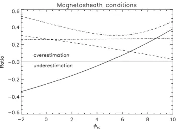
Fig. 4. Estimation ratios as in Fig. 3 but for the magnetosheath case: rN (solid line),rv(dashed line), rT (dot-dashed line). The
upper curve is the estimation indexIe.
Fig. 5. Estimation ratios as in Fig. 3 but for the magnetosphere case: rN (solid line),rv(dashed line), rT (dot-dashed line). The
upper curve is the estimation indexIe.
the case where the spacecraft potential and the lower energy cutoff are equal. The range spanned by the velocity and tem-perature is much smaller; however, the velocity measure can reach a 75% overestimation for zero potential.
Fig. 6. Minimal density overestimationrN for potentials higher
than the detector cutoff (taken here as 10 eV), i.e.√−E> vl, in the
solar wind case (solid line), the magnetosheath case (dashed line) and the magnetosphere case (dot-dashed line).
overestimation varies from 30 to a few percent. The density measure is still most affected by the spacecraft potential and varies from a 25% underestimation (for zero potential) to a 37% overestimation.
The variations ofIe, the estimation index, agree with the
above conclusions. For solar wind conditions, this index is close to 1, indicating that the potential has a great ef-fect on the measure (Ie=1 corresponds, for instance, to an
under/over-estimation of 60% on the three moments). This value is much less in the magnetosheath and magnetosphere. Also, the minimum of this index occurs for potentials close to the critical potential (for which N0=N) which typically lies in the range 2–6 V, the higher value corresponding to the solar wind. This range agrees well with the capabili-ties of existing active potential control devices as employed, for example, on Polar (PSI experiment, Moore et al. (1995), with a bias potential∼2 V) and Cluster (ASPOC experiment, Torkar et al., 2001, with a bias potential∼3–7 V). Such de-vices basically emit a positive ion beam to counter the posi-tive charge and manage to dynamically stabilize the potential to values close to the bias value.
What happens when the spacecraft potential reaches val-ues higher than the lower energy cutoff? This situation, as far as distribution functions are concerned, is illustrated on the lower panel of Fig. 2. Photoelectrons can now freely enter the detector. However, these particles are not taken into ac-count in our model. The algorithm still works but in the range
vl<v<
√
−E we set f=0, suppressing the photoelectrons which we do not model. This explains the kinks in the varia-tions of the different ratios occuring at the location√−E=vl,
as shown in Fig. 6. Therefore, for√−E>vl, in the case of
the density, for instance, our method does not give the proper overestimation in the measure, but rather the minimal overes-timation, as in a real case, photoelectrons would further add to the density value. We discussed in Sect. 2 how photoelec-trons might generally be modeled. Thus, in Fig. 6 we display the minimal density overestimation for different plasma
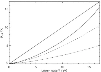
con-Fig. 7. Critical potential as a function of the lower cutoff of the detector, in the solar wind case (solid line), the magnetosheath case (dashed line) and the magnetosphere case (dot-dashed line).
ditions. For larger potentials (such that√−E>vl), the trends, previously described for different plasma regimes, are still present. For instance,8sc=20 V (andmev2l/2=10 eV) leads
to a 15% minimal overestimation for magnetospheric condi-tions, emphasizing the low dependence of the moments on the spacecraft potential in this region, whereas in the mag-netosheath case this value reaches 100%. In the solar wind, the overestimation quickly reaches high values (more than 300%). However, in the low density environment, such as the solar wind, the spacecraft potential rarely attains values above 10 eV used as the lower energy cutoff in Fig. 6.
For zero potential, the overestimation (usually occurring for the velocity and temperature measurements) is a 3-D ef-fect. Indeed, in 1-D, when there is no integration over the an-gular part, the integrand for all moments is strictly positive, and the truncation due to the low energy cutoff can only lead to underestimation. In 3-D the integrand for the moments may be negative at low velocities (see Eq. 12, for instance); the truncation then misses this part and gives a larger result than the total integration (vl=0, vu=∞). Trying to sketch
1-D plots for this problem may thus be misleading. The ef-fect of the potential increase is to bring more of the negative integrand area into the sampling (or integration) range. This explains why the velocity is less overestimated at larger po-tential. As the temperature is the combination of three differ-ent pressure terms divided by the density, it is more difficult to discriminate exactly how the (usually small) overestima-tion occurs.
In Fig. 7 we no longer keep the lower cutoff constant to study its effect on the moment estimation, and more specifi-cally, on the critical potential8crit previously defined. This
quantity is a relevant parameter which bounds the density under/over-estimation regions. Therefore, for a given lower cutoff, when the spacecraft potential is smaller (larger) than
8crit the density will be under(over)estimated. In a region
in the solar wind the variations are large. Indeed, an increase of the lower cutoff involves smaller relative undersampling for a broad distribution than for a peaked one. Therefore, one needs a smaller increase of the potential to shift the dis-tribution in energy and obtain equality between the measured and real density. Small variations of the lower cutoff have a strong implication on the density estimation, at least in the solar wind where the spacecraft potential rarely exceeds 10 V: for a cutoff value of 10 eV both under and overesti-mation can be expected, whereas for a value of 15 eV only underestimation is possible as8crit≃12 V. In the solar wind
casee8crit quickly reaches values larger than the lower
cut-off which is a domain where our model is not complete (pho-toelectrons are lacking).
5 Conclusions
Revisiting the “perfect” detector concept, we expressed ana-lytically the “measured” moments (density, velocity and tem-perature) as functions of the (a priori unknown) moments of a Maxwellian distribution function in free space, the space-craft potential, and lower and upper energy cutoffs of the de-tector. We numerically inverted the complex nonlinear sys-tem derived from the previous equations, and finally obtained the “real” moments. This enabled us to estimate what is the influence of the spacecraft potential by comparing real and instrumentally determined measured moments. Let us sum-marize the basic findings of the present paper.
– The corrections due to the potential can be very impor-tant, especially in the solar wind and magnetosheath environments, by comparison with the case 8sc=0 V
(Song et al., 1997).
– The model shows that the active control of the space-craft potential to values less than 10 V minimizes to some extent the discrepancies between real and mea-sured moments. This is due to the offsetting effects of the low energy instrumental cutoff and the residual po-tential.
– The value of the lower cutoff has significant influence on the estimation of the density, as shown by the varia-tions of the critical potential8crit.
Several lines could be followed to improve the existing model:
– The model of the detector geometry could be improved in the method (see Scime et al., 1994, for instance), al-though this would destroy the angular symmetry which permitted several simplifying analytical steps.
– Fore8sc>mevl2/2, the contribution of the
photoelec-trons could be added. Such a situation happens when the plasma density is very low (the lobes, for instance). This requires a correct model of the photoelectron dis-tribution to be implemented (see, for instance, Grard, 1973; Pedersen, 1995).
– A potential barrier outside the spacecraft (a few space-craft radii away) exists when the photoelectrons dom-inate the space charge around it. This barrier may af-fect the plasma measurements in an equivalent way as raising the lower energy cutoff. Both plasma and photo-electron distributions are then modified. However, this non-monotonic potential behaviour is difficult to deter-mine (see, for instance, Whipple, 1976; Thi´ebault et al., 2004).
– As the method is partly numerical, it would be possible to assume distribution functions other than Maxwellian. Anisotropies related to the magnetic field direction would again break the angular symmetry and increase the numerical complexity.
However, any improvement will not change the basic fea-ture of the method: it deals with pre-computed moments which may be affected by calibration deficiency (energy effi-ciency, geometry factor, etc.). In the complex process of cor-recting moments from spacecraft potential and energy cut-offs, it may then be more valuable to use data from a lower level, namely to work directly with the distribution functions. For instance, it is possible to apply a potential correction di-rectly to the 3-D distribution functions by shifting the energy channels of the corresponding energy, and then recompute the moments from these new distributions; any holes left in the distributions may be filled by some simple model fit. If this seems the most obvious solution, it often does not of-fer a good alternative as the 3-D products from an energy spectrometer cannot always be transmitted with high time resolution to the ground (they require too much telemetry). The result is then, at best, moments with degraded time res-olution. A fix to this problem could be to perform a similar method using the pitch-angle distributions which are gener-ally transmitted at a higher rate. However, this is done at the expense of invoking an assumption of gyrotropy. In conclu-sion, no perfect method to correct spacecraft potential effects has been designed yet, and the one presented in this paper, with its limitations but with also its simplicity, can provide a crude and quick improvement from the measured moments to their underlying true values.
Acknowledgements. V. G´enot is supported by a UK PPARC grant. Topical Editor T. Pulkkinen thanks G. Paschmann for his help in evaluating this paper.
References
Bouhram, M., Dubouloz, N., Hamelin, M., Grigoriev, S. A., Malin-gre, M., Torkar, K., Veselov, M. V., Galperin, Y., Hanasz, J., Per-raut, S., Schreiber, R., and Zinin, L. V.: Electrostatic interaction between Interball-2 and the ambient plasma, 1. Determination of the spacecraft potential from current calculations Ann. Geophys., 20, 365, 2002.
and Wave Analyser: Performances and Perspectives for the Clus-ter Mission, Space Sci. Rev., 79, 157, 1997.
Forest, J., Eliasson, L., and Hilgers, A.: A New Spacecraft Plasma Simulation Software, PicUp3D/Spis, 7th Spacecraft Charging and Technology Conference, p.515–520, ESA/SP-476, ESA-ESTEC, Noordwijk, The Netherlands, 23–27 April 2001. Grard, R. J. L: Properties of the satellite photoelectron sheath
de-rived from photoemission laboratory measurements, J. Geophys. Res., 78, 2885, 1973.
Hilgers, A., Holback, B., Holmgren, G., and Bostrom, R.: Probe measurements of low plasma densities with applications to the auroral acceleration region and auroral kilometric radiation sources, J. Geophys. Res., 97, 8631, 1992.
Johnstone, A. D., Alsop, C., Burge, S., Carter, P. J., Coates, A. J., Coker, A. J., Fazakerley, A. N., Grande, M., Gowen, R. A., Gurgiolo, C., Hancock, B. K., Narheim, B., Preece, A., Sheather, P. H., Winningham, J. D., and Woodliffe, R. D.: Peace: a Plasma Electron and Current Experiment, Space Sci. Rev., 79, 351, 1997. Laakso, H. and Pedersen, A.: Ambient electron density derived from differential potential measurements, Measurement Tech-niques in Space Plasmas, edited by Borovsky, J., Pfaff, R., and Young, D., AGU Monograph 102, 49, AGU, Washington DC, 1998.
Lin, R. P., Anderson, K. A., Ashford, S., Carlson, C., Curtis, D., Ergun, R., Larson, D., McFadden, J., McCarthy, M., Parks, G. K., R`eme, H., Bosqued, J. M., Coutelier, J., Cotin, F., D’Uston, C., Wenzel, K.-P., Sanderson, T. R., Henrion, J., Ronnet, J. C., and Paschmann, G.: A Three-Dimensional Plasma and Energetic Particle Investigation for the Wind Spacecraft, Space Sci. Rev., 71, 125, 1995.
Meyer-Vernet, N., Hoang, S., Issautier, K., Maksimovic, M., Man-ning, R., Moncuquet, M., and Stone, R. G.: Measuring plasma parameters with thermal noise spectroscopy, Measurement Tech-niques in Space Plasmas, edited by Borovsky, J., Pfaff, R., and Young, D., AGU Monograph 102, 205, AGU, Washington DC, 1998.
Moore, T. E., Chappell, C. R., Chandler, M. O., Fields, S. A., Pol-lock, C. J., Reasoner, D. L., Young, D. T., Burch, J. L., Eaker, N., Waite Jr., J. H., McComas, D. J., Nordholt, J. E., Thomsen, M. F., Berthelier, J. J., and Robson, R.: The Thermal Ion Dynamics Experiment and Plasma Source Instrument, Space Sci. Rev., 71, 409, 1995.
Paschmann G., Fazakerley, A. N., and Schwartz, S. J.: Moments of plasma velocity distributions, Analysis Methods for Multi-Spacecraft Data, Chapter 6, edited by Paschmann, G. and Daly, P. W., ISSI scientific report, 1998.
Pedersen, A.: Solar wind and magnetosphere plasma diagnostics by spacecraft electrostatic potential measurements, Ann. Geophys., 13, 118, 1995.
Press, W. H., Teukolsky, S. A., Vetterling, W. T., and Flannery, B. P.: Numerical Recipes in Fortran 77: The Art of Scientific Com-puting, Cambridge University Press, 1992.
Salem, C., Bosqued, J.-M., Larson, D. E., Mangeney, A., Maksi-movic, M., Perche, C. , Lin, R. P., and Bougeret, J.-L.: Determi-nation of accurate solar wind electron parameters using particle detectors and radio wave receivers, J. Geophys. Res., 106, 10, 21 701, 2001.
Scime, E. E., Phillips, J. L., and Barne, S. J.: Effects of spacecraft potential on three-dimensional electron measurements in the so-lar wind, J. Geophys. Res., 99, 8, 14 769, 1994.
Singh, N., Leung, W. C., Moore, T. E., and Craven, P. D.: Numer-ical model of the plasma sheath generated by the plasma source instrument aboard the Polar satellite, J. Geophys. Res., 106, 9, 19 179, 2001.
Song, P., Zhang, X. X., and Pashmann, G.: Uncertainties in plasma measurements: effect of lower cutoff energy and spacecraft charge, Planet. Space Sci., 45, 2, 255, 1997.
Szita, S., Fazakerley, A. N., Carter, P. J., James, A. M., Tr´avn´ıˇcek, P., Watson, G., Andr´e, M., Eriksson, A., and Torkar, K.: Clus-ter PEACE observations of electrons of spacecraft origin, Ann. Geophys., 19, 1, 2001.
Thi´ebault, B., Hilgers, A., Sasot, E., Laakso, H., Escoubet, P., G´enot, V., and Forest, J.: Potential barrier in the electrostatic sheath around a magnetospheric spacecraft, J. Geophys. Res., ac-cepted, 2004.
Torkar, K., Riedler, W., Escoubet, C. P., Fehringer, M., Schmidt, R., Grard, R. J. L., Arends, H., F. R¨udenauer, Steiger, W., Narheim, B. T., Svenes, K., Torbert, R., Andr´e, M., Fazakerley, A., Gold-stein, R., Olsen, R. C., Pedersen, A., Whipple, E., and Zhao, H.: Active spacecraft potential control for Cluster – implementation and first results, Ann. Geophys., 19, 1289, 2001.