Regional albedo of Arctic first-year drift ice in advanced stages of melt from the combination of in situ measurements and aerial imagery

(1)

TCD

8, 3699–3732, 2014

Arctic first-year ice albedo during summer melt from

aerial surveys

D. V. Divine et al.

Title Page

Abstract Introduction

Conclusions References

Tables Figures

◭ ◮

Back Close

Full Screen / Esc

Printer-friendly Version

Interactive Discussion

Discussion

P

a

per

|

Discus

sion

P

a

per

|

Discussion

P

a

per

|

Discussion

P

a

per

|

The Cryosphere Discuss., 8, 3699–3732, 2014 www.the-cryosphere-discuss.net/8/3699/2014/ doi:10.5194/tcd-8-3699-2014

This discussion paper is/has been under review for the journal The Cryosphere (TC). Please refer to the corresponding final paper in TC if available.

Regional albedo of Arctic first-year drift

ice in advanced stages of melt from the

combination of in situ measurements and

aerial imagery

D. V. Divine, M. A. Granskog, S. R. Hudson, C. A. Pedersen, T. I. Karlsen, S. A. Divina, and S. Gerland

Norwegian Polar Institute, FRAM Centre, 9296 Tromsø, Norway

Received: 17 June 2014 – Accepted: 22 June 2014 – Published: 11 July 2014

Correspondence to: D. V. Divine (dmitry.divine@npolar.no)

(2)

TCD

8, 3699–3732, 2014

aerial surveys

D. V. Divine et al.

Title Page

Tables Figures

◭ ◮

Back Close

Full Screen / Esc

Discussion

P

a

per

|

Discus

sion

P

a

per

|

Discussion

P

a

per

|

Discussion

P

a

per

|

Abstract

The paper presents a case study of the regional (_≈150 km) broadband albedo of first year Arctic sea ice in advanced stages of melt, estimated from a combination of in situ albedo measurements and aerial imagery. The data were collected during the eight day ICE12 drift experiment carried out by the Norwegian Polar Institute in the Arctic

5

north of Svalbard at 82.3◦N from 26 July to 3 August 2012. The study uses in situ albedo measurements representative of the four main surface types: bare ice, dark melt ponds, bright melt ponds and open water. Images acquired by a helicopter borne camera system during ice survey flights covered about 28 km2. A subset of >8000 images from the area of homogeneous melt with open water fraction of _≈0.11 and

10

melt pond coverage of≈0.25 used in the upscaling yielded a regional albedo estimate of 0.40 (0.38; 0.42). The 95 % confidence interval on the estimate was derived using the moving block bootstrap approach applied to sequences of classified sea ice im-ages and albedo of the four surface types treated as random variables. Uncertainty in the mean estimates of surface type albedo from in situ measurements contributed

15

some 95 % of the variance of the estimated regional albedo, with the remaining vari-ance resulting from the spatial inhomogeneity of sea ice cover. The results of the study are of relevance for the modeling of sea ice processes in climate simulations. It par-ticularly concerns the period of summer melt, when the optical properties of sea ice undergo substantial changes, which existing sea ice models have significant diffuculty

20

accurately reproducing.

1 Introduction

A new thin-ice Arctic system requires reconsideration of the set of parameterizations of mass and energy exchange within the ocean–sea ice–atmosphere system used in modern coupled general circulation models (CGCMs) including Earth System Models

25

(3)

measure-TCD

8, 3699–3732, 2014

aerial surveys

D. V. Divine et al.

Title Page

Tables Figures

◭ ◮

Back Close

Full Screen / Esc

Discussion

P

a

per

|

Discus

sion

P

a

per

|

Discussion

P

a

per

|

Discussion

P

a

per

|

ments made specifically on first-year pack ice with a focus on the summer melt season, when the difference from typical conditions for the earlier multi-year Arctic sea ice cover becomes most pronounced (Perovich and Polashenski, 2012).

Surface albedo is one of the major physical quantities controlling the intensity of the energy exchange at the atmosphere–sea ice–ocean interface and the heat balance of

5

sea ice (e.g. Doronin and Kheisin, 1977; Maykut, 1982; Curry et al., 1995). Knowledge of the surface albedo for different types of sea ice, as well as its spatial and seasonal variability, is crucial for obtaining an adequate representation of the sea-ice cycle in CGCMs (Holland et al., 2012; Karlsson and Svensson, 2013).

During summer, the net positive heat balance of sea ice causes substantial

trans-10

formation in the state of the ice cover. Water runo_fffrom melting snow and upper ice layers tends to form puddles in depressions in the sea ice surface (e.g. Zubov, 1945; Untersteiner, 1961; Nazintsev, 1964). These melt ponds spread rapidly and on level first year ice can cover up to 70 % of the surface during the initial stage of surface melt (Polashenski et al., 2012). As the albedo of a melt pond is markedly lower than that

15

of the bare or snow-covered sea ice (e.g. Doronin and Kheisin, 1977; Perovich et al., 2002), the spatial distribution of melt ponds and leads has clear implications for the spatial aggregate albedo and accelerated summer decay of sea ice.

Field observations suggest a pronounced difference in the seasonal evolution of first-year sea-ice albedo compared with that of multifirst-year ice. The surface of multifirst-year sea

20

ice typically features more rough topography and thicker snow cover, leading to a lim-ited potential melt pond coverage (e.g. Perovich and Polashenski, 2012). Thicker ice underneath the melt pond bottom leads to generally higher spatial albedo, lower trans-mission and energy absorption of melting multiyear ice (Hudson et al., 2013; Nicolaus et al., 2012). As a result, the summer albedo of multiyear ice cover is systematically

25

higher than that of younger ice throughout the entire melt season, inducing an addi-tional ice age–albedo feedback (Perovich and Polashenski, 2012).

(4)

TCD

8, 3699–3732, 2014

aerial surveys

D. V. Divine et al.

Title Page

Tables Figures

◭ ◮

Back Close

Full Screen / Esc

Discussion

P

a

per

|

Discus

sion

P

a

per

|

Discussion

P

a

per

|

Discussion

P

a

per

|

pond coverage, and the overcast conditions prevailing in the summer Arctic promote the use of low-altitude airborne methods for studying the morphological and optical properties of the sea ice cover. Combining these with in situ measurements of inci-dent/reflected solar radiation (albedo) and turbulent heat fluxes for different types of surfaces may in turn provide estimates of the regional-scale surface energy balance of

5

sea ice. A number of such studies have been conducted in the past with a focus on spatial and temporal evolution of fractional melt pond coverage, pond-size probability density (see e.g. Perovich et al., 2002 for a review), and their relationship with the pre-melt surface topography (Derksen et al., 1997; Petrich et al., 2012). Depending on the instrumentation setup used, the spatial ranges covered varied from tens of meters to

10

hundreds of kilometers, on the order of the typical scale of a GCM grid cell.

A comprehensive set of observations of the energy balance of melting Arctic first-year sea ice was conducted during an eight-day ice station in July–August 2012. Hud-son et al. (2013) presented results from in situ measurements obtained during the drift experiment. This paper shows the analysis of the regional morphological properties of

15

the sea-ice surface, inferred from aerial surveys. The in situ measurements of broad-band albedo and the derived regional spatial distribution of surface types are used to obtain an estimate of the regional albedo of Arctic first-year ice in the advanced stages of melt.

Section 2 presents the geographical settings, instrument setup, image processing

20

techniques used in the study, and uncertainties in the key variables we used for esti-mating the regional albedo. Section 3.1 shows the spatial variability of melt pond and open water fractions inferred from six helicopter ice survey flights. Details on the up-scaling technique applied, along-track albedo variability, and regional albedo estimates are then presented in Sect. 3.2. Finally the results of the work are discussed and

sum-25

(5)

TCD

8, 3699–3732, 2014

aerial surveys

D. V. Divine et al.

Title Page

Tables Figures

◭ ◮

Back Close

Full Screen / Esc

Discussion

P

a

per

|

Discus

sion

P

a

per

|

Discussion

P

a

per

|

Discussion

P

a

per

|

2 Data and methods

2.1 ICE12 drift experiment

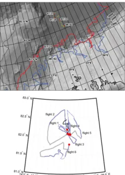
The energy balance of melting thin first-year Arctic sea ice was a focus of the eight-day ICE12 drifting ice floe experiment on R/VLance, conducted 26 July to 3 August 2012 north of Svalbard, in the southwestern Nansen Basin (82.3◦N, 21.5◦E). Figure 1 shows

5

theLancedrift track that was in an area of very close (_≥90 %) drift ice, see operational ice charts from the Norwegian Ice Service for reference (www.met.no). The ice floe (ICE12 floe hereafter) thatLancewas moored to during the drift had a size of approx-imately∅600 m and a modal ice thickness of 0.8 m, from drillings and measurements using a Geonics EM-31 electromagnetic induction device (Hudson et al., 2013). Based

10

on airborne surveys of ice thickness using another electromagnetic induction device, the EM-bird (Haas et al., 2009), and aerial photography, it was found to be representa-tive for the area. The sea ice was in the latter stages of melt, with some of the ponds actually melted through the ice slab.

The imaging of the sea-ice surface during the cruise was done using a recently

de-15

signed ICE camera system mounted on a Eurocopter AS-350 helicopter. The hardware component of the system includes two downward looking Canon EOS 5D Mark II digi-tal photo cameras equipped with Canon 20 mm f/2.8 USM lenses, a combined SPAN-CPT GPS/INS unit by Novatel, and a laser distance measurement device LDM301 by Jenoptik used as an altimeter in the setup. These components were housed in a single

20

aerodynamic enclosure and mounted outside the helicopter. The single-point horizon-tal positioning accuracy for the system was within 1.5 m, and the uncertainty in the altitude over the sea ice was estimated to be<0.3 m, which corresponds to a typical scale of sea ice draft variability.

Since the ICE camera was designed as a component of a photogrammetric setup,

25

(6)

TCD

8, 3699–3732, 2014

aerial surveys

D. V. Divine et al.

Title Page

Tables Figures

◭ ◮

Back Close

Full Screen / Esc

Discussion

P

a

per

|

Discus

sion

P

a

per

|

Discussion

P

a

per

|

Discussion

P

a

per

|

30–40 m s−1– parameters typical for EM-bird flights. We fixed the camera lenses’ focal lengths to infinity. For every captured image, the position, attitude, and altitude of the event were logged in the system. The cameras’ own 128 GB compact flash cards stored the captured images; the card size was sufficient for the system to shoot continuously for about an hour, taking about 4500 images per camera in raw Canon format. A subset

5

of some 10 300 images with minimal (<10 %) or no overlap captured during six longer survey flights was selected for further processing and used in the presented study. To form this subset, every second image from one of the cameras was used. Figure 1 shows the selected flight tracks. Results of the data analysis from these flights together with in situ observations are reported below and also summarized in Table 1.

10

2.2 Image and navigation data processing

For a typical flight altitude of about 35 m over the sea ice, the camera lenses used in the setup provide a footprint of about 60 by 40 m. With the CCD geometry at its native resolution this corresponds to a pixel size on the ground of about 1 cm. For typical helicopter roll (pitch) angles of about₋2◦(1◦) the distortion of the image plane from an

15

ideal rectangular one and the associated uncertainty in the image area of less than 1 % was considered insignificant; therefore no correction for pitch and roll was applied to the images.

Image correction for camera lens distortion is necessary prior to any further analysis of the acquired images. We used a generic lens correction and vignetting correction

20

procedures implemented in®Adobe Lightroom software.

In order to discriminate between open water, bare ice, and melt ponds, we applied a three-step object identification and classification procedure. This involved:

a. image segmentation/binarization using Otsu’s method, which chooses the thresh-old to minimize the intra-class variance of the black and white pixels (Otsu, 1979)

25

(7)

TCD

8, 3699–3732, 2014

aerial surveys

D. V. Divine et al.

Title Page

Tables Figures

◭ ◮

Back Close

Full Screen / Esc

Discussion

P

a

per

|

Discus

sion

P

a

per

|

Discussion

P

a

per

|

Discussion

P

a

per

|

c. object classification (open water, bare ice or melt pond) using thresholding in the red channel intensity.

Due to the relatively high contrast between the different surface types during summer melt, this relatively simplistic approach appeared to work well with a minimum of su-pervision required during the processing of the sequences of images captured by the

5

camera system. All procedures were implemented in Matlab using the “Image process-ing” toolbox (MATLAB, 2012).

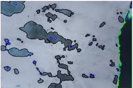
Figure 2 demonstrates an example of the object classification procedure for an image captured during flight 1 (Table 1). The edges of the melt pond objects are accurately identified. Note that we left out the darker objects with an area less than 0.5 m2, as the

10

contribution of these objects to the total melt pond coverage was found to be negligi-ble. The identified set of objects of three types is then used for calculating summary statistics on melt pond coverage and open water fraction. The parts of the image not classified as melt ponds or open water were considered as bare sea ice. For the case in Fig. 2 the open water fraction (fow) was calculated to be 8 % and the fractional melt

15

pond coverage (fmp) was 16 % with respect to the total sea-ice area.

2.3 Aggregate albedo

Hudson et al. (2013) used a di_fferent surface type classification technique from Renner et al. (2013) that additionally discriminated between two types of melt ponds on the sea ice surface: dark and bright ponds. The latter refers to light blue ponds with thicker,

20

more reflective ice underneath. The broadband albedo of these three sea-ice surface types was measured in situ during the ICE12 drift experiment using a mobile instrument platform for measuring the radiation budget on sea ice (Hudson et al., 2012, 2013). In the estimates that follow we use the ratio of “dark” to “bright” pond areas, r =2.8, determined from the additional analysis of 859 randomly selected images from flight

25

(8)

TCD

8, 3699–3732, 2014

aerial surveys

D. V. Divine et al.

Title Page

Tables Figures

◭ ◮

Back Close

Full Screen / Esc

Discussion

P

a

per

|

Discus

sion

P

a

per

|

Discussion

P

a

per

|

Discussion

P

a

per

|

white iceαbi=0.55 (see Table 1 in Hudson et al., 2013 for more details and Supplement

Table S1 presented here). The albedo of open water/leads is set to the commonly usedαow=0.066 (Pegau and Paulson, 2001). We note that cloudy conditions prevailed

during the drift experiment, ensuring relative homogeneity in illumination in the study area.

5

The aggregate albedo is generally defined as (Perovich, 2005):

α=g(αj,fj) := X

j

αjfj;αj,fj ∈[0, 1] (1)

where summation is over all surface types used, herej={ow, bi, bp, dp_}, with the cor-responding fractional coveragef_j. Note that for convenience we use the fractional total

10

melt pond coverage fmp with relation to the sea-ice area. Coefficientsfbp and fdp are

defined as fractions of bright and dark melt ponds with regard to the relative melt pond coverage, i.e.fbp=(1/(1+r))fmpandfdp=(r/(1+r))fmp. This transforms Eq. (1) forα

to

α=αowfow+αbi(1−fmp)(1−fow)+αbpfbp(1−fow)+αdpfdp(1−fow) (2)

15

For example, the fractional melt pond coverage offmp=16 %, with respect to sea ice

area, and open water fraction of 4 % of the 0.95 km2of the ICE12 floe area yields an aggregate albedo of about 0.48.

In this study, the values of open-water and melt-pond fractions, the areal ratio of

20

(9)

TCD

8, 3699–3732, 2014

aerial surveys

D. V. Divine et al.

Title Page

Tables Figures

◭ ◮

Back Close

Full Screen / Esc

Discussion

P

a

per

|

Discus

sion

P

a

per

|

Discussion

P

a

per

|

Discussion

P

a

per

|

2.4 Accounting for uncertainties in the variables used

2.4.1 Error models for melt ponds and open water fractional coverage

Error models on the fractional coverage of open water and melt ponds are built on the additional analysis of 859 images from flight 2 using the classification method of Ren-ner et al. (2013). The technique involves a semi-automated surface type classification

5

and manual supervision of the processed images, allowing more reliable results at the cost of increased labour intensity. Processing of the images used in this verification procedure yielded the image-based fractional coverage of the four surface classes: dark ponds, bright ponds, open water or leads, and bare ice. This dataset was used as a reference to estimate the uncertainty in the corresponding quantities derived from

10

the larger image set and to assess the probability density of the ratio of the areas of dark to bright ponds at the regional scale.

Imagewise intercomparison offmp and fow values demonstrated an average bias of

fb=0.04 withσfb=0.05 in the fraction of melt ponds between the images processed using the technique of Renner et al. (2013) and the simplified approach applied in

15

this study. Inspection of images revealed that the algorithm presented in Sect. 2.2 sometimes underestimates the melt pond coverage by identifying some bright ponds as bare white ice. Likewise, some of the darkest melt ponds were sometimes misidentified as open water/leads. The error model forfmpi andfowi of an imagei is therefore defined

as

20

n p f_mpi

,p f_owi o

=

 

 p fmpi

∼pfmpi +N f b

,σ_f2b

|N fb,σ_f2b

≥0

p fowi

∼pfowi −(1−f

i

ow)N f b

,σ_f2b

|N fb,σ_f2b

<0 (3)

where parameters of the Gaussian distribution were estimated from the data.

The areal ratio of dark to bright pondsr was estimated using a bootstrap technique (Efron and Tibshirani, 1993) involving sampling with replacement from the same

com-25

(10)

TCD

8, 3699–3732, 2014

aerial surveys

D. V. Divine et al.

Title Page

Tables Figures

◭ ◮

Back Close

Full Screen / Esc

Discussion

P

a

per

|

Discus

sion

P

a

per

|

Discussion

P

a

per

|

Discussion

P

a

per

|

for each bootstrap replicate. The proportion of the drawn to replaced data points (i.e. classified images) within each replicate was set to 2/1 with all the images being equally weighted. The resulting distribution of the mean arealr derived from 10 000 replicates was approximated by a Gaussian probability density function withp(r)_{∼ N}(2.8, 0.152).

2.4.2 In situ broadband albedo as a random variable 5

Uncertainties in the average in situ albedoαj are estimated empirically from available

data for each surface typej. During the ICE12 experiment we obtained 50 individual albedo measurements over bare white ice, 12 over dark melt ponds, and 1 over a bright pond. This yields sample standard deviationsσ_αspon single point measurements of 0.05 and 0.04 for bare white ice and dark ponds, respectively (see Supplement Table S1 for

10

details). Using a simplistic error model assuming independent measurements with ran-dom Gaussian errors, we calculate the uncertainty of the measurement-based average albedo of surface typejas

σ_α_j =

σ_αsp_j p_m j

+

σ_αins_j p_m j

(4)

15

wheremj refers to the number of available albedo measurements in the surface type

under consideration. The single measurement instrumental errorσ_αins_j was set to 0.1α_j, where the coe_fficient 0.1 stems from a declared 5 % measurement uncertainty yielding a total uncertainty of 10 % for the ratio of reflected to incoming radiation (i.e. albedo), again assuming the errors are independent. For the “bright pond” category, where only

20

one albedo measurement was available with no significant influence from other surface types, we assigned an uncertainty of 0.1αbp although we acknowledge that this value

(11)

TCD

8, 3699–3732, 2014

aerial surveys

D. V. Divine et al.

Title Page

Tables Figures

◭ ◮

Back Close

Full Screen / Esc

Discussion

P

a

per

|

Discus

sion

P

a

per

|

Discussion

P

a

per

|

Discussion

P

a

per

|

mean albedo of every surface type j can now be considered as a t distributed ran-dom variable withmj degrees of freedom, distributed as p(αj)∼αj+tm_jσα_j. The use

oft distribution accounts for a larger spread in the estimate of the true mean when dealing with the relatively small sample sizes. For bright ponds, the Gaussian approxi-mation was used instead to prevent the occasional generation of albedo values outside

5

the admissible range of [0, 1] due to heavy tails of thet distribution with one degree of freedom.

This approach should be considered a simplification, as it reduces the whole variety of surface types with different optical chartacteristic to only four major surface types. However we expect that the imposed range of random variability in a particular

surface-10

type albedo covers the natural variation of this parameter, thereby accounting indirectly for the effects of numerous additional factors like the thickness of ice, surface state and small scale morphology, pond depth and ice thickness beneath the pond as well as changing light conditions.

3 Results and discussion 15

3.1 Spatial variability of melt pond coverage and open water inferred from helicopter surveys

This section presents the results of the analysis of sea ice imagery along the six se-lected flights tracks that took place during the ICE12 cruise (Table 1). All but one flight (flight 1, on 31 July) were combined EM-bird/ICE camera flights, which fixed the

heli-20

copter flight altitude to approximately 35 m above the sea-ice surface, except for some shorter periods of climbing to 150–200 m for EM-bird calibration. During the calibra-tion the helicoper typically hovered above the same locacalibra-tion and only a few images captured during the calibrations were retained for the analysis.

Figures 3 and 4 show the summary statistics of melt pond and sea ice/open water

25

(12)

TCD

8, 3699–3732, 2014

aerial surveys

D. V. Divine et al.

Title Page

Tables Figures

◭ ◮

Back Close

Full Screen / Esc

Discussion

P

a

per

|

Discus

sion

P

a

per

|

Discussion

P

a

per

|

Discussion

P

a

per

|

presented in Supplement Figs. S1, S3, S5, and S7. For five of six flights, those carried out from 31 July to 2 August, the results are similar, with a typical fractional melt pond coveragefmpof about 25 % and a similarity in the shapes of the respective probability

density distributions. The open water fractionfow varies between 7 and 13 %, but this

variability lies within the uncertainty of the mean estimates and corresponds well to the

5

respective operational ice charts for the area.

Flight 6, on 3 August, was conducted while moving southwards out of the close drift ice. The flight track traversed the marginal ice zone (MIZ) with extensive areas/strips of open water. Thus the estimates offow(30 %) andfmp(20 %) for flight 6 are substantially

different from those inferred from survey flights conducted the previous days in the

10

close pack ice (see Fig. 4).

3.2 Estimating regional albedo from in situ measurements and helicopter borne imagery

3.2.1 Bootstrapping to upscale the local albedo measurements to a regional scale

15

The results of in situ measurements from the ICE12 drift experiment are further up-scaled to assess the regional scale albedo in the study area using the flight-track data of surface-type distribution, more specifically the series of _{fmpi ,f

i

ow,S

i

}, i =1,. . .,N, with Si standing for the respective area of image i. Figures 5a and 6a show local (i.e. based on individual images) aggregate albedo estimatesαi made from the

heli-20

copter imagery along the two selected flights with the contrasting surface conditions presented in Sect. 3.1. The results for other tracks are presented in Supplement and further summarized in Table 1. Note that in this case the image-based albedo variability is estimated from the data treated “as is” without taking the uncertainties into account. Figure 5b and corresponding figures in the Supplement demonstrate fairly similar

25

(13)

approxi-TCD

8, 3699–3732, 2014

aerial surveys

D. V. Divine et al.

Title Page

Tables Figures

◭ ◮

Back Close

Full Screen / Esc

Discussion

P

a

per

|

Discus

sion

P

a

per

|

Discussion

P

a

per

|

Discussion

P

a

per

|

mately 80 km of the ICE12 floe. We note that the empirical probability density functions (pdf) of local albedo are skewed substantially towards zero, due to the contribution of open water areas. This suggests that an estimate of the regional scale surface albedo of melting sea ice pack made by simple averaging of the respective quantities from a sequence of local scenes can be negatively biased. This may have implications for

5

areal estimates of the surface energy budget, both in observational and modeling stud-ies. Moreover, as in the case of any random variable with an a priori unknown theoret-ical distribution, the accuracy of the parameters of its empirtheoret-ical estimate is related to the availalbe data sample.

The whole swath-based aggregate albedoαsis therefore calculated in the same way

10

as the local estimates using Eq. (2), with the values offows andf s

mpderived as

f_ows =X

i

Sif_owi . X i

Si

fmps =

X

i

Si 1₋fowi

fmpi

. X

i Si

and referring to the swath-based estimates of open water and melt pond fractions.

15

Since the probability distribution of the local, image-based albedo αi, is non-Gaussian, the large number of available samples makes the bootstrapping (i.e. sam-pling with replacement) technique (Efron and Tibshirani, 1993) an optimal choice to assess the accuracy of the estimated swath albedo. The presence of autocorrelation in the data suggests the use of the moving block bootstrap approach (Kunsch, 1989).

20

For each flight the application of this method to the sequence of_{fowi ,f

i

mp,S

i

}involves the following steps:

1. The series of_{fowi ,f

i

mp,S

i

}of lengthN is split intoN₋K+1 overlapping blocks of lengthK; the block length is determined empirically from the data, the procedure is described in the next subsection.

(14)

TCD

8, 3699–3732, 2014

aerial surveys

D. V. Divine et al.

Title Page

Tables Figures

◭ ◮

Back Close

Full Screen / Esc

Discussion

P

a

per

|

Discus

sion

P

a

per

|

Discussion

P

a

per

|

Discussion

P

a

per

|

2. N/K blocks are drawn at random, with replacement, from the constructed set of

N₋K+1 blocks, and their sequence numbers are registered.

3. Mbootstrap samples are drawn from the subset ofN/K blocks; albedo for the four different surface types and the values forfowi ,fmpi andr can at this step be drawn

at random from the respective probability distributions defined in Sects. 2.4.1 and

5

2.4.2; the swath-based albedoαsis then calculated for each sample using Eq. (2). Steps 2–3 are repeatedLtimes to generateL_·Mestimates of the swath-based aggre-gate albedoαs. The assigned values of _{L,M}=200 yield a total of 40 000 samples of αs which is sufficient for minimizing the effect of random sampling errors. Panels c in Figs. 5, 6 and Supplement Figs. S2, S4, S6, S8 display the generated bootstrap

10

probability density of the swath-based αs for the six flights. The 95 % confidence in-terval (CI0.95) on each estimated swath-based albedo is then calculated as {2.5, 97.5}

percentiles of the emprirical bootstrap pdf ofαs. Table 1 shows the calculated values of the average swath-based albedos and their respective bootstrap CI_0.95. For all tracks the αs probality density is approximately Gaussian, with 95 % confidence according

15

to the Lilliefors goodness-of-fit test of composite normality (Conover, 1999). The re-spective fits are shown together with the bootstrap pdfs in Figs. 5, 6 and Supplement Fig. S2, S4, S6 and S8. The standard deviations of the fitted Gaussian distributions are

σ_αs =0.01 for flights 1–5 andσ_αs

6=0.02 for flight 6.

The five similar flight tracks demonstrate similar values of the swath-based aggregate

20

albedoαs, all lying within the estimated confidence intervals (see Fig. 7). This suggests the data from these five flights can be combined to provide the regional-scale estimate of the surface albedo. This is implemented using the same technique applied to the concatenated sequence of _{fmpi ,f

i

ow,S

i

}for all flight tracks but flight 6. The latter was not included in calculations of the regional estimate due to a substantially different state

25

(15)

TCD

8, 3699–3732, 2014

aerial surveys

D. V. Divine et al.

Title Page

Tables Figures

◭ ◮

Back Close

Full Screen / Esc

Discussion

P

a

per

|

Discus

sion

P

a

per

|

Discussion

P

a

per

|

Discussion

P

a

per

|

In order to infer the relative contribution of the spatial variability in melt pond/open water coverage and the uncertainty of in situ albedo measurements to the overall vari-ance of the swath-based and regional albedo estimates, we repeated the numerical experiments, with the albedo of surface types treated as constants. The result demon-strated a substantial reduction in standard deviation ofσαs to 0.003 andσ_αr to 0.002.

5

This indicates that in the defined framework about 90 % of the estimated variance of

αs and 95 % in αr is due to variability and uncertainties in the in situ albedo mea-surements. Only a minor part of the variance is due to all other errors and variability accounted for in the model.

3.2.2 Estimating the image block lengthK using the Markov chain 10

Accounting for the autocovariance in the analyzed data is implemented following the Nychka et al. (2000) modification of the Mitchell et al. (1966) formula

N_e_ff=N1−φ−0.68/ √

N

1+φ+0.68/√N, (5)

whereNeff stands for the effective number of degrees of freedom (“effective sample 15

size”); in general,Neff< N due to the presence of autocorrelation in a series. This

ap-proach implicitly assumes that the analyzed sequence can be adequately described as a realization of the discrete first order autoregressive process with the autoregressive parameterφ.

For each classified imagei treated as an individual data sample, further

categoriza-20

tion into “ice” or “open water” was applied. Such binarization into the two major surface classes is related to their dominant contribution to the swath-based albedo variance. The images within one flight track that have both open water and sea ice were cate-gorized using a threshold in local open water fraction. The value for the thresholdfowt

was set to 5 %, which for the typical flight altitude would correspond to an opening in

25

(16)

TCD

8, 3699–3732, 2014

aerial surveys

D. V. Divine et al.

Title Page

Tables Figures

◭ ◮

Back Close

Full Screen / Esc

Discussion

P

a

per

|

Discus

sion

P

a

per

|

Discussion

P

a

per

|

Discussion

P

a

per

|

Fitting the Markov chain of first order to the derived binary sequence of surface states comprising one complete flight yields the transition matrixT. Its largest entry, which in our case characterizes the likelihood of retaining the “ice” state between two successive images, was used as the sought parameterφ– a simplistic metric of spatial autocorrelation in the surface state for the analyzed flight track. The resulting values

5

ofφ varied in the range of 0.78–0.88, whereas the probability of retaining the “open water” state was lower, 0.51–0.57. These results are summarized in Table 2. The block lengthK was then calculated as a ratio ofN/Neff, yielding a block size of 9–12 images

for four of the six transects, which correspondeds to approximately 500–700 m of the flight track. For the tracks with the lowest (flight 1) and highest (flight 6) open water

10

fractions the derived block lengths were 18 and 7 images, respectively.

3.2.3 Assessing the aggregate scale for ICE camera imagery

The notion of aggregate scale for an environmental variable refers to the minimal spa-tial scale at which the contribution of local sampling variability to its total variance is diminished (Moritz et al., 1993). The concept is directly related to the weak law of

15

large numbers, provided that the samples are drawn from a stationary distribution. Knowledge of this scale is crucial for an accurate upscaling of local measurements and subsequently linking them to larger-scale climate models. We note that in a hierarchy of spatial scales the present study focuses specifically on the range of meters to hun-dreds of kilometers that encompasses the scales typical for in situ measurements up

20

to regional and CGCM models.

The aggregate scale for the regional albedo was estimated using sets of (pseudo)-independent samples of different size drawn from the whole collection of classified im-ages. The sample size varied from 10 to 1000 images, and for each sample size 10 000 subsets were drawn at random, without replacement, to gain the necessary statistics

25

(17)

TCD

8, 3699–3732, 2014

aerial surveys

D. V. Divine et al.

Title Page

Tables Figures

◭ ◮

Back Close

Full Screen / Esc

Discussion

P

a

per

|

Discus

sion

P

a

per

|

Discussion

P

a

per

|

Discussion

P

a

per

|

area over 6000 m2, corresponding to a flight altitude above 55 m, were not included in the analysis.

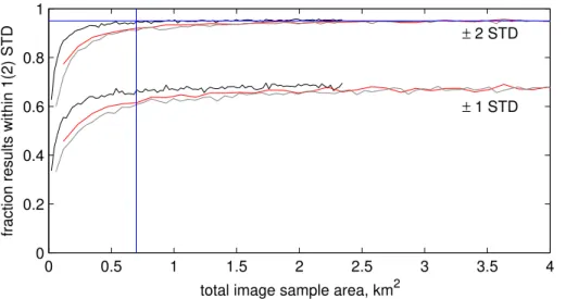
Figure 8 (black lines) shows the fraction of sample-based aggregate albedo esti-mates falling within the interval of_±1 and _±2 standard deviations of the regional ag-gregate albedo (Table 1), as a function of sample area. The results demonstrate a rapid

5

growth in the proportion of accurate estimates of the regional albedo with an increase in the number of images drawn for analysis. The curves level out when the total sample area exceeds the threshold of about 0.7 km2, when some 95 % of the subset based estimates lie within the interval of 2 STD of the regional bootstrap albedo. One should emphasize that these estimates are specific to this study’s setup, time period and

re-10

gion. For the range of flight altitudes typically sustained during the operation of the EM-bird, the 0.7 km2aggregate scale corresponds to a set of at least 300 independent images spatially representative of the study region.

In order to simulate higher flight altitudes and examine the effect of smaller sample sets and/or sub-kilometer scale spatial autocorrelation in the state of sea ice cover on

15

the estimate of the aggregate scale, the numerical experiment was repeated with suc-cessive images combined into blocks of different length. The validity of this experiment relies on the assumption of smaller scale anisotropy in statistical properties of the sea ice surface. The red and gray lines in Fig. 8 show the fraction of the accurate estimates of the regional albedo for image blocks of length 10 and 25 images, respectively.

Re-20

sults suggest an increase in the aggregate scale to values above 2 km2 which would correspond to sets of at least 80 (30) area-representative images captured from an al-titude of about 100 (170) m. Notably the estimated thresholds (aggregate scales) have an order of magnitude similar to the respective estimate of about 1 km2 obtained by Perovich et al. (2002) during the SHEBA experiment in a different region of the Arctic.

(18)

TCD

8, 3699–3732, 2014

aerial surveys

D. V. Divine et al.

Title Page

Tables Figures

◭ ◮

Back Close

Full Screen / Esc

Discussion

P

a

per

|

Discus

sion

P

a

per

|

Discussion

P

a

per

|

Discussion

P

a

per

|

4 Conclusions

The formation of smaller scale features such as melt ponds on summer sea ice entirely alters its optical properties over a broad range of wavelengths. This has implications for the surface energy balance and summer sea ice decay as well as for practical is-sues of the remote sensing of sea ice. The study of sea ice topography and associated

5

processes at these smaller scales is therefore of crucial importance for a better un-derstanding of the seasonal evolution of the ice pack at a pan-Arctic scale. Yet consid-erable regional and intraseasonal variability of summer first-year ice albedo stipulates the need for further regional scale studies of this parameter and its relation to other key physical factors characterizing the current state of sea ice cover.

10

Safety and logistical challenges associated with these types of studies result in the relevant field data preferentially representing thicker first-year sea ice at the ini-tial stages of melt and/or sea ice from coastal areas, where the sediment load may modify the spectral albedo and melt pattern. Limited data exist for thinner, less than 1 m thick, Arctic first-year ice that is expected to occupy a substantial part of the Arctic

15

basin in the future when (and if) the projected transition to a nearly seasonal ice cover has occurred.

Analysis of imagery from five of six low-altitude (35–40 m) ice survey flights during the ICE12 drift experiment north of Svalbard at 82.3◦N in late July–early August 2012 revealed a regional scale homogeneity in melt pond coverage and open water fraction

20

in the area of the drift track outside the MIZ. Within this area, with an extent of_≈150 km, the observed melt pond fraction varied from 15–36 % in 50 % of cases, around the mean of fmpi =26 % relative to the sea ice area. In some occasions the melt ponds

covered as much as 66 % of the ice surface, yet for some 10 % of images with sea ice in the field of view the sea ice surface exhibited no or very little melt pond coverage

25

(fmpi <4 %). The average open water fraction of f

i

ow=11 % was characteristic of very

(19)

TCD

8, 3699–3732, 2014

aerial surveys

D. V. Divine et al.

Title Page

Tables Figures

◭ ◮

Back Close

Full Screen / Esc

Discussion

P

a

per

|

Discus

sion

P

a

per

|

Discussion

P

a

per

|

Discussion

P

a

per

|

As surface characteristics exhibit pronounced spatial variability at this range of scales, data inferred from individual low-altitude images must be considered as sam-ples drawn from some random field with an a priori unknown distribution. Any result inferred from the entire dataset is therefore only an estimate, and the confidence inter-val on this estimate is to be provided. We used the block bootstrapping technique to

5

account for uncertainties due to sampling in the spatial domain, surface type classifi-cation errors, and in situ albedo measurements used in the upscaling procedure. The set of more than 8000 classified images representing a total of 21 km2, combined with a series of in situ broadband albedo measurements conducted on sea ice, was used to produce the regional aggregate albedo estimate of 0.40 (0.38; 0.42). The bootstrap

10

albedo for flight 6, conducted within the MIZ, shows a lower value of 0.34 (0.31; 0.37) due to a higher open water fraction, 30 %. Notably the melt pond fraction of about 20 % observed during this flight was lower too. We speculate this is related to the smaller floe size and ice thickness in the MIZ promoting more e_fficient lateral drainage and percolation of melt ponds.

15

The use of a large collection of classified images from the area allowed an assess-ment of the aggregate scale for the regional albedo of about 0.7 km2which corresponds to at least 300 images captured by the ICE camera setup from an altitude of 35–40 m. Higher flight altitudes would require fewer classified images, though the area covered must be larger. We emphasize that these estimates are linked with the setup

configu-20

ration used as well as the state of sea-ice cover during the ICE12 experiment.

The regional scale of this work and the relatively short time period covered com-plicate a comparison with similar studies on the topic. Analysis of the relevant liter-ature indicates that our albedo estimates are systematically lower than the spatially averaged albedo of melting FYI reported in a number of other ship-based/aerial

stud-25

(20)

substan-TCD

8, 3699–3732, 2014

aerial surveys

D. V. Divine et al.

Title Page

Tables Figures

◭ ◮

Back Close

Full Screen / Esc

Discussion

P

a

per

|

Discus

sion

P

a

per

|

Discussion

P

a

per

|

Discussion

P

a

per

|

tial interannual/intraseasonal variability in surface conditions, including the prevalent ice type, melt pond and open water fractions, and the values of albedos for specific surface types used in upscaling to a regional aggregate estimate. A typical example is seen in the results of Lu et al. (2010), which report a much lower (less than 15 %) area fraction of melt ponds on sea ice observed along their cruise track in summer

5

2008. In the latitudes similar to our study this was however compensated by a much higher (>40 %) open water fraction, yielding aggregate albedo estimates similar to this work. Higher ice concentrations,>80 %, were observed farther north. The end of the melt season, associated with the onset of surface freeze up, however caused a low melt pond coverage (Lu et al., 2010) that kept the estimated albedo at a level higher

10

than was esimated in this work. We note also that the current study was carried out on thinner sea ice, hence with darker melt ponds, which led to lower albedos for these two surface types and hence a lower regional albedo estimate compared with the similar values used in the aforementioned studies.

Our results indicate that about 95 % of the uncertainty in the regional albedo estimate

15

as it was defined in our framework is due to variability in the in situ albedo measure-ments. This variability is related to both the natural local variability of this parameter due to, e.g. underlying ice thickness or pond depth, as well as the uncertainty stem-ming from the measurement technique itself. This indicates the need for a series of local measurements carried out for each surface category as a necessary prerequisite

20

for a high quality regional uspcaling. A particular focus should be on melt pond albedo evolution at the latter stages of ice decay, when the ice beneath the ponds gets thin, the ponds begin to melt through, and their albedo approaches that of open water.

Further processing and analysis of the data from 2012 is an ongoing effort. The plans for further work include detailed analysis of the spatial melt pond distribution and

25

(21)

TCD

8, 3699–3732, 2014

aerial surveys

D. V. Divine et al.

Title Page

Tables Figures

◭ ◮

Back Close

Full Screen / Esc

Discussion

P

a

per

|

Discus

sion

P

a

per

|

Discussion

P

a

per

|

Discussion

P

a

per

|

The Supplement related to this article is available online at doi:10.5194/tcd-8-3699-2014-supplement.

Acknowledgements. We thank the crew of R/VLanceandAirliftas well as other scientists and

engineers on board for their assistance in carrying out the measurements. Funding was pro-vided by the Centre for Ice, Climate and Ecosystems (ICE) at the Norwegian Polar Institute via

5

the ICE-Fluxes project. This work was also supported by ACCESS, a European Project within the Ocean of Tomorrow call of the European Commission Seventh Framework Programme, grant 265863, and the Research Council of Norway through the EarthClim (207711/E10) project.

References 10

Conover, W.: Practical Nonparametric Statistics, Wiley Series in Probability and Statistics, 3rd Edn., Wiley, New York, 1999. 3712

Curry, J. A., Schramm, J. L., and Ebert, E. E.: Sea ice-albedo climate feedback mechanism, J. Climate, 8, 240–247, doi:10.1175/1520-0442(1995)008<0240:SIACFM>2.0.CO;2, 1995. 3701

15

Derksen, C., Piwowar, J., and LeDrew, E.: Sea-ice melt-pond fraction as determined from low level aerial photographs, Arctic Alpine Res., 29, 345–351, 1997. 3702

Doronin, Y. and Kheisin, D.: Sea Ice, Amerind Publishing Company, Office of Polar Programs and the National Science Foundation, Washington DC, 1977. 3701

Efron, B. and Tibshirani, R. J.: An Introduction to the Bootstrap, Chapman & Hall, New York,

20

1993. 3707, 3711

Gonzalez, R.: Digital Image Processing Using MATLAB, McGraw-Hill Education, India, Pvt Lim-ited, 2010. 3704

Haas, C., Lobach, J., Hendricks, S., Rabenstein, L., and Pfaffling, A.: Helicopter-borne mea-surements of sea ice thickness, using a small and lightweight, digital EM system, J. Appl.

25

Geophys., 67, 234–241, doi:10.1016/j.jappgeo.2008.05.005, 2009. 3703

(22)

TCD

8, 3699–3732, 2014

aerial surveys

D. V. Divine et al.

Title Page

Tables Figures

◭ ◮

Back Close

Full Screen / Esc

Discussion

P

a

per

|

Discus

sion

P

a

per

|

Discussion

P

a

per

|

Discussion

P

a

per

|

Holland, M. M., Bailey, D. A., Briegleb, B. P., Light, B., and Hunke, E.: Improved sea ice short-wave radiation physics in CCSM4: the impact of melt ponds and aerosols on arctic sea ice, J. Climate, 25, 1413–1430, doi:10.1175/JCLI-D-11-00078.1, 2012. 3701

Hudson, S. R., Granskog, M. A., Karlsen, T. I., and Fossan, K.: An integrated platform for observing the radiation budget of sea ice at different spatial scales, Cold Reg. Sci. Technol.,

5

82, 14–20, doi:10.1016/j.coldregions.2012.05.002, 2012. 3705

Hudson, S. R., Granskog, M. A., Sundfjord, A., Randelhoff, A., Renner, A. H. H., and Di-vine, D. V.: Energy budget of first-year Arctic sea ice in advanced stages of melt, Geophys. Res. Lett., 40, 2679–2683, doi:10.1002/grl.50517, 2013. 3701, 3702, 3703, 3705, 3706 Karlsson, J. and Svensson, G.: Consequences of poor representation of Arctic sea-ice albedo

10

and cloud-radiation interactions in the CMIP5 model ensemble, Geophys. Res. Lett., 40, 4374–4379, doi:10.1002/grl.50768, 2013. 3701

Kunsch, H. R.: The jackknife and the bootstrap for general stationary observations, Ann. Stat., 17, 1217–1241, doi:10.1214/aos/1176347265, 1989. 3711

Lu, P., Li, Z., Cheng, B., Lei, R., and Zhang, R.: Sea ice surface features in Arctic summer 2008:

15

aerial observations, Remote Sens. Environ., 114, 693–699, doi:10.1016/j.rse.2009.11.009, 2010. 3717, 3718

MATLAB: Version 8.0.0.783 (R2012b), The MathWorks Inc., Natick, Massachusetts, 2012. 3705

Maykut, G.: Large-scale heat exchange and ice production in the Central Arctic, J. Geophys.

20

Res., 87, 7971–7984, 1982. 3701

Mitchell, J., Dzerdzeevskii, B., and Flohn, H.: Climatic Change: Report of a Working Group of the Commission for Climatology, Technical Note 79, World Meteorological Organisation, 1966. 3713

Moritz, R. E., Curry, J., Thorndike, A., and Untersteiner, N.: SHEBA: A Research Program on

25

the Surface Heat Budget of the Arctic Ocean, Report 3, Arctic Syst. Sci.: Ocean-Atmos.-Ice Interact., University of Washington, Seattle, 34 pp., 1993. 3714

Nazintsev, Y.: The heat balance of the surface of the multiyear ice cover in the central Arctic, Trudy AANII, 267, 110–126, 1964 (in Russian). 3701

Nicolaus, M., Katlein, C., Maslanik, J., and Hendricks, S.: Changes in Arctic sea ice

re-30

(23)

TCD

8, 3699–3732, 2014

aerial surveys

D. V. Divine et al.

Title Page

Tables Figures

◭ ◮

Back Close

Full Screen / Esc

Discussion

P

a

per

|

Discus

sion

P

a

per

|

Discussion

P

a

per

|

Discussion

P

a

per

|

Nychka, D., Buchberger, R., Wigley, T., Santer, B. D., Taylor, K. E., and Jones, R. H.: Con-fidence intervals for trend estimates with autocorrelated observations, available at: http:// citeseerx.ist.psu.edu/viewdoc/download?doi=10.1.1.33.6828&rep=rep1&type=pdf (last ac-cess: 8 July 2014), unpublished manuscript, 2000. 3713

Otsu, N.: A threshold selection method from gray-level histograms, IEEE T. Syst. Man Cyb., 9,

5

62–66, doi:10.1109/TSMC.1979.4310076, 1979. 3704

Pegau, S. W. and Paulson, C. A.: The albedo of Arctic leads in summer, Ann. Glaciol., 33, 221–224, doi:10.3189/172756401781818833, 2001. 3706, 3708

Perovich, D. K.: On the aggregate-scale partitioning of solar radiation in Arctic sea ice during the Surface Heat Budget of the Arctic Ocean (SHEBA) field experiment, J. Geophys.

Res.-10

Oceans, 110, C03002, doi:10.1029/2004JC002512, 2005. 3706

Perovich, D. K. and Polashenski, C.: Albedo evolution of seasonal Arctic sea ice, Geophys. Res. Lett., 39, L08501, doi:10.1029/2012GL051432, 2012. 3701

Perovich, D. K., Tucker, W. B., and Ligett, K. A.: Aerial observations of the evolu-tion of ice surface condievolu-tions during summer, J. Geophys. Res.-Oceans, 107, 8048,

15

doi:10.1029/2000JC000449, 2002. 3701, 3702, 3715, 3717

Perovich, D. K., Grenfell, T. C., Light, B., Elder, B. C., Harbeck, J., Polashenski, C., Tucker, W. B., and Stelmach, C.: Transpolar observations of the morphological properties of Arctic sea ice, J. Geophys. Res.-Oceans, 114, C00A04, doi:10.1029/2008JC004892, 2009. 3717

Petrich, C., Eicken, H., Polashenski, C. M., Sturm, M., Harbeck, J. P., Perovich, D. K., and

20

Finnegan, D. C.: Snow dunes: a controlling factor of melt pond distribution on Arctic sea ice, J. Geophys. Res.-Oceans, 117, C09029, doi:10.1029/2012JC008192, 2012. 3702

Polashenski, C., Perovich, D., and Courville, Z.: The mechanisms of sea ice melt pond formation and evolution, J. Geophys. Res.-Oceans, 117, C01001, doi:10.1029/2011JC007231, 2012. 3701

25

Renner, A. H., Dumont, M., Beckers, J., Gerland, S., and Haas, C.: Improved characterisation of sea ice using simultaneous aerial photography and sea ice thickness measurements, Cold Reg. Sci. Technol., 92, 37–47, doi:10.1016/j.coldregions.2013.03.009, 2013. 3705, 3707 Tschudi, M. A., Curry, J. A., and Maslanik, J. A.: Airborne observations of summertime surface

features and their effect on surface albedo during FIRE/SHEBA, J. Geophys. Res., 106,

30

15335, doi:10.1029/2000JD900275, 2001. 3717

(24)

TCD

8, 3699–3732, 2014

aerial surveys

D. V. Divine et al.

Title Page

Tables Figures

◭ ◮

Back Close

Full Screen / Esc

Discussion

P

a

per

|

Discus

sion

P

a

per

|

Discussion

P

a

per

|

Discussion

P

a

per

|

World Meteorological Organization: WMO Sea-Ice Nomenclature, Terminology, Codes and Illustrated Glossary, 1970 Edn., Secretariat of the World Meteorological Organization, Geneva, 1970. 3713

Zubov, N.: Arctic Ice, Izd. Glavsevmorputi, Moscow, 1945 (translated by US Navy Oceano-graphic Office, Springfield, 1963). 3701

(25)

TCD

8, 3699–3732, 2014

aerial surveys

D. V. Divine et al.

Title Page

Tables Figures

◭ ◮

Back Close

Full Screen / Esc

Discussion

P

a

per

|

Discus

sion

P

a

per

|

Discussion

P

a

per

|

Discussion

P

a

per

|

Table 1.Summary statistics on the state of sea ice cover and aggregate surface albedo along the six processed helicopter flight tracks from ICE12 cruise. The open water coveragefows ,

melt pond fractionf_mps (relative to sea ice area) and albedo values presented are the whole swath-based estimates rather than averages of the respective values from individual images presented in the corresponding figures. The regional aggregate scale albedo is calculated in the same way from the whole dataset less flight 6. The numbers in parentheses in the albedo column denote the respective block bootstrap 95 % confidence interval on the estimates.

Flight Date GMT start-end Nimages Transect length fs

ow, % fmps, % Aggregate

(26)

TCD

8, 3699–3732, 2014

aerial surveys

D. V. Divine et al.

Title Page

Tables Figures

◭ ◮

Back Close

Full Screen / Esc

Discussion

P

a

per

|

Discus

sion

P

a

per

|

Discussion

P

a

per

|

Discussion

P

a

per

|

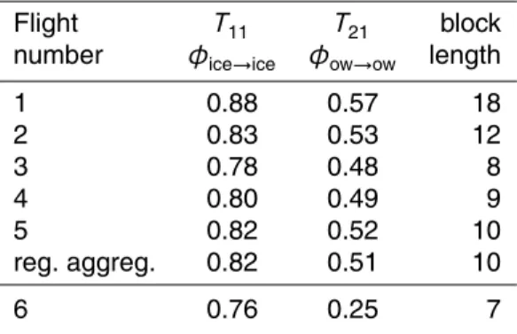
Table 2.Auxiliary data for the processed flight tracks used in calculation of the flight track albedo. T₁₁ and T₂₁ denote elements of the transition matrix of the fitted first order Markov model and the respective estimated image block lengths.

Flight T₁₁ T₂₁ block

number φ_ice_→_ice φ_ow_→_ow length

1 0.88 0.57 18

2 0.83 0.53 12

3 0.78 0.48 8

4 0.80 0.49 9

5 0.82 0.52 10

reg. aggreg. 0.82 0.51 10

(27)

TCD

8, 3699–3732, 2014

aerial surveys

D. V. Divine et al.

Title Page

Tables Figures

◭ ◮

Back Close

Full Screen / Esc

Discussion

P

a

per

|

Discus

sion

P

a

per

|

Discussion

P

a

per

|

Discussion

P

a

per

|

(28)

TCD

8, 3699–3732, 2014

aerial surveys

D. V. Divine et al.

Title Page

Tables Figures

◭ ◮

Back Close

Full Screen / Esc

Discussion

P

a

per

|

Discus

sion

P

a

per

|

Discussion

P

a

per

|

Discussion

P

a

per

|

(29)

TCD

8, 3699–3732, 2014

aerial surveys

D. V. Divine et al.

Title Page

Tables Figures

◭ ◮

Back Close

Full Screen / Esc

Discussion

P

a

per

|

Discus

sion

P

a

per

|

Discussion

P

a

per

|

Discussion

P

a

per

|

a

16.0° E 20.0° E 24.0° E

82.0° N 82.5°_N

83.0° N

flight 2 01.08.2012

0 0.25 0.5 0.75 1

0 1 2 3 4 5

prob.density

melt pond fraction

b

flight distance, km

fractional coverage

c

0 20 40 60 80 100 120 140

0 0.2 0.4 0.6 0.8 1

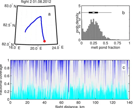
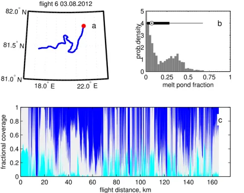
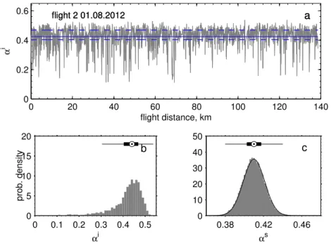
Figure 3.Data summary from flight 2 on 1 August 2012, 07:23–08:35 UTC;(a)flight track with photo coverage;(b)empirical probability density of fractional melt pond coveragefmpalong the

flight track relative to sea ice; image-based meanfmpof 25 % and the quartilesQ1,2,3of 15, 25

and 34 %, respectively, as shown by the Box plot; image averagedf_ow9 %. The whiskers on Box plot highlight the 1.5 times interquartile range to cover some 99 % of the observations in total;

(c)fractional melt pond coveragef_mp(light blue), bare icef_bi(light grey) and open water fraction

(30)

TCD

8, 3699–3732, 2014

aerial surveys

D. V. Divine et al.

Title Page

Tables Figures

◭ ◮

Back Close

Full Screen / Esc

Discussion

P

a

per

|

Discus

sion

P

a

per

|

Discussion

P

a

per

|

Discussion

P

a

per

|

a

18.0° E 22.0° E

81.0° N 81.5° N

82.0°_N

flight 6 03.08.2012

0 0.25 0.5 0.75 1

0 1 2 3 4 5

prob.density

melt pond fraction b

flight distance, km

fractional coverage

c

0 20 40 60 80 100 120 140 160

0 0.2 0.4 0.6 0.8 1

(31)

TCD

8, 3699–3732, 2014

aerial surveys

D. V. Divine et al.

Title Page

Tables Figures

◭ ◮

Back Close

Full Screen / Esc

Discussion

P

a

per

|

Discus

sion

P

a

per

|

Discussion

P

a

per

|

Discussion

P

a

per

|

0 20 40 60 80 100 120 140

0 0.2 0.4 0.6

flight distance, km

α

i

flight 2 01.08.2012 a

0 0.1 0.2 0.3 0.4 0.5

0 5 10 15 20

prob. density

αi

b

0.38 0.42 0.46

0 10 20 30 40 50

αs

c

(32)

TCD

8, 3699–3732, 2014

aerial surveys

D. V. Divine et al.

Title Page

Tables Figures

◭ ◮

Back Close

Full Screen / Esc

Discussion

P

a

per

|

Discus

sion

P

a

per

|

Discussion

P

a

per

|

Discussion

P

a

per

|

0 20 40 60 80 100 120 140 160

0 0.2 0.4 0.6

flight distance, km

α

i

flight 6 03.08.2012 a

0 0.1 0.2 0.3 0.4 0.5

0 5 10 15 20

prob. density

αi

b

0.25 0.3 0.35 0.4 0.45

0 10 20 30 40 50

αs

c

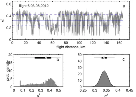
Figure 6.Same as in Fig. 5 but for flight 6 shown in Fig. 4. Solid blue line is for the image-based track average albedo of 0.32, dashed lines show the 25 and 75 percentiles (0.23,0.42) of the respectiveαi probability density shown in(b);(c)bootstrap swath-based aggregate albedoαs