Fine particulate matter source apportionment using a hybrid chemical transport and receptor model approach

(1)

ACPD

13, 26657–26698, 2013

A hybrid approach to source

apportionment

Y. Hu et al.

Title Page

Abstract Introduction

Conclusions References

Tables Figures

◭ ◮

Back Close

Full Screen / Esc

Printer-friendly Version

Interactive Discussion

Discussion

P

a

per

|

D

iscussion

P

a

per

|

Discussion

P

a

per

|

Discuss

ion

P

a

per

|

Atmos. Chem. Phys. Discuss., 13, 26657–26698, 2013 www.atmos-chem-phys-discuss.net/13/26657/2013/ doi:10.5194/acpd-13-26657-2013

Atmospheric Chemistry and Physics

Open Access

Discussions

This discussion paper is/has been under review for the journal Atmospheric Chemistry and Physics (ACP). Please refer to the corresponding final paper in ACP if available.

Fine particulate matter source

apportionment using a hybrid chemical

transport and receptor model approach

Y. Hu1, S. Balachandran1, J. E. Pachon1,*, J. Baek1,**, C. Ivey1, H. Holmes1, M. T. Odman1, J. A. Mulholland1, and A. G. Russell1

1

School of Civil and Environmental Engineering, Georgia Institute of Technology, Atlanta, Georgia, USA

*

now at: Program of Environmental Engineering, Universidad de La Salle, Bogota, Colombia

**

now at: Center for Global and Regional Environmental Research, University of Iowa, Iowa City, Iowa, USA

Received: 31 August 2013 – Accepted: 18 September 2013 – Published: 15 October 2013

Correspondence to: Y. Hu ([email protected])

(2)

ACPD

13, 26657–26698, 2013

apportionment

Y. Hu et al.

Title Page

Tables Figures

◭ ◮

Back Close

Full Screen / Esc

Discussion

P

a

per

|

D

iscussion

P

a

per

|

Discussion

P

a

per

|

Discuss

ion

P

a

per

|

Abstract

A hybrid fine particulate matter (PM2.5) source apportionment approach based on a receptor-model (RM) species balance and species specific source impacts from a chemical transport model (CTM) equipped with a sensitivity analysis tool is devel-oped to provide physically- and chemically-consistent relationships between source

5

emissions and receptor impacts. This hybrid approach enhances RM results by pro-viding initial estimates of source impacts from a much larger number of sources than are typically used in RMs, and provides source-receptor relationships for secondary species. Further, the method addresses issues of source collinearities, and accounts for emissions uncertainties. Hybrid method results also provide information on the

re-10

sulting source impact uncertainties. We apply this hybrid approach to conduct PM2.5 source apportionment at Chemical Speciation Network (CSN) sites across the US. Ambient PM_2.5concentrations at these receptor sites were apportioned to 33 separate sources. Hybrid method results led to large changes of impacts from CTM estimates for sources such as dust, woodstove, and other biomass burning sources, but limited

15

changes to others. The refinements reduced the differences between CTM-simulated and observed concentrations of individual PM2.5 species by over 98 % when using a weighted least squared error minimization. The rankings of source impacts changed from the initial estimates, revealing that CTM-only results should be evaluated with ob-servations. Assessment with RM results at six US locations showed that the hybrid

20

results differ somewhat from commonly resolved sources. The hybrid method also re-solved sources that typical RM methods do not capture without extra measurement information on unique tracers. The method can be readily applied to large domains and long (such as multi-annual) time periods to provide source impact estimates for management- and health-related studies.

25

(3)

ACPD

13, 26657–26698, 2013

apportionment

Y. Hu et al.

Title Page

Tables Figures

◭ ◮

Back Close

Full Screen / Esc

Discussion

P

a

per

|

D

iscussion

P

a

per

|

Discussion

P

a

per

|

Discuss

ion

P

a

per

|

1 Introduction

Fine particulate matter (PM2.5) with an aerodynamic diameter less than 2.5 µm is asso-ciated with adverse effects on human health (Dockery et al., 1993). From the perspec-tive of linking health e_ffects with air quality, and for assessing air quality management options, it is desirable to have the spatially and temporally resolved impacts of

ma-5

jor emission sources. However, quantifying the impacts of all individual sources on the ambient concentration of fine particulate matter, better known as source apportionment (SA), is challenging. A fundamental issue with any SA method is that there is no way to directly measure source impacts, and, as such, it is difficult to assess the accuracy of source apportionment results. Tracer gases such as cyclic perfluoroalkanes and SF₆

10

can be utilized to help quantify source impacts (Martin et al., 2011). However, that is far from measuring multiple sources’ impacts at the same time and is typically limited to special studies. Instead, source apportionment results are typically evaluated by com-paring simulated concentrations of individual component and total mass of PM2.5with observations.

15

Receptor model (RM) approaches have long been used for PM_2.5source apportion-ment (Chow et al., 1992; Cooper and Watson, 1980; Liu et al., 2006; Martello et al., 2008; Reffet al., 2007; Schauer et al., 1996; Swietlicki et al., 1996; Thurston et al., 2011; Viana et al., 2008b; Watson, 1984; Watson et al., 2008; Xie et al., 2013). These methods, such as the Chemical Mass Balance (CMB) (Watson et al., 1984) or Positive

20

Matrix Factorization (PMF) (Pattero and Tapper, 1994), rely on using observed species concentrations of PM_2.5at a receptor(s) and solve a set of species balance equations to estimate source impacts. RM methods typically do not use emissions estimates or ex-plicitly account for the chemical and physical processes that governs pollutant transport and transformation after being emitted from a specific source. To address them,

addi-25

(4)

ACPD

13, 26657–26698, 2013

apportionment

Y. Hu et al.

Title Page

Tables Figures

◭ ◮

Back Close

Full Screen / Esc

Discussion

P

a

per

|

D

iscussion

P

a

per

|

Discussion

P

a

per

|

Discuss

ion

P

a

per

|

order of ten out of hundreds in the inventory), comprising about 80 % of the estimated emissions (Baek, 2009), leading to potential biases in the results. In RM methods, the common approach for assessing the accuracy of source apportionment results is to compare the calculated PM_2.5 composition concentrations and total mass to observa-tions, and if they compare well, it is assumed that the results are reasonable. However,

5

this type of evaluation does not use a set of observations that are totally independent from the ones used to obtain the source impacts, although non-fitting species compar-ison and other tests can be used to assist in the evaluation (USEPA, 2004). Further, similar estimated species concentrations, and hence similar performance, can result from very different combinations of source impacts. Results can also be quite sensitive

10

to model inputs (e.g., source profiles for CMB), or the number of sources (or factors in PMF) used. Differences in source apportionment results for similar cases found be-tween competing RM methods also suggest errors (Held et al., 2005; Laupsa et al., 2009; Lee et al., 2008; Lowenthal et al., 2010; Marmur et al., 2006; Rizzo and Sche_ff, 2007; Shi et al., 2009; Viana et al., 2008a; Watson et al., 2008). Several studies have

15

tried to reconcile the results by refining source profiles and adding extra constraints (Lee and Russell, 2007; Marmur et al., 2007; Sheesley et al., 2007; Swietlicki et al., 1996; Watson et al., 2008). Extra species such as organic molecular markers and other unique tracers for certain sources have been utilized in RM modeling (Bullock et al., 2008; Lee et al., 2009; Schauer et al., 1996; Zheng et al., 2002) to improve the

accu-20

racy and identify additional sources, however measurements of those markers are not available on routine monitoring networks.

Source-oriented modeling (SM) approaches, such as chemical transport models (CTMs), follow the emission, transport, transformation and loss of chemical species in the atmosphere to simulate ambient concentrations and source impacts. CTMs can

25

compensate for limitations in RM methods (Burr and Zhang, 2011a, b; Doraiswamy et al., 2007; Held et al., 2005; Henze et al., 2009; Kleeman et al., 2007; Lowenthal et al., 2010; Marmur et al., 2006; Russell, 2008; Schichtel et al., 2006; Wagstrom et al., 2008; Ying et al., 2008) because they describe processes affecting source-receptor

(5)

ACPD

13, 26657–26698, 2013

apportionment

Y. Hu et al.

Title Page

Tables Figures

◭ ◮

Back Close

Full Screen / Esc

Discussion

P

a

per

|

D

iscussion

P

a

per

|

Discussion

P

a

per

|

Discuss

ion

P

a

per

|

relationships from a first principles basis. For example, compared with RMs, CTMs di-rectly account for secondary formation of PM2.5and nonlinearities in pollutant transfor-mations and have the ability to quantify a more complete range of sources. Also, CTMs use knowledge of the specific location of emission sources in the region and their emission rates and can provide spatially resolved source impacts across the modeling

5

domain. An important strength of using CTMs for source apportionment is that model evaluation relies on independent data. However, estimates of source strengths and characteristics (e.g., diurnal and day-to-day variations) are viewed as highly uncertain, meteorological inputs of CTMs contain errors, and there continue to be uncertainties in how various processes are described. Due to these uncertainties and the effort

in-10

volved, the application of SM approaches for source apportionment is limited.

One way to take the advantages of SM approaches is to further improve SM source apportionment results by utilizing species concentration observations in a manner sim-ilar to RM approaches. Here, a hybrid SM-RM approach is developed and applied to obtain improved source impact estimates by integrating measurements with the CTM

15

results, including uncertainty estimates of measurements and emissions. As devel-oped, the method integrates the CMB method with CTM results at monitoring locations and measurement times, by adding additional information and constraints in a species balance approach similar to CMB. The improved source impact estimates at these sparse locations can potentially be utilized to obtain source impact fields using spatial

20

and temporal interpolation that take advantage of the initial CTM estimates across the domain and over the time period of interest. In this study the hybrid approach is applied to a 36 km resolution CTM simulation over North America. Our focus is to demonstrate the hybrid method by closely examining SM-RM source apportionment results across all sites and with more detail at select locations.

(6)

ACPD

13, 26657–26698, 2013

apportionment

Y. Hu et al.

Title Page

Tables Figures

◭ ◮

Back Close

Full Screen / Esc

Discussion

P

a

per

|

D

iscussion

P

a

per

|

Discussion

P

a

per

|

Discuss

ion

P

a

per

|

2 Methods

2.1 CTM simulation and measurement data

Simulated three-dimensional concentration fields of trace chemical species are ob-tained using the Community Multiscale Air Quality model (CMAQ) (Byun and Schere, 2006) version 4.5 with strict mass conservation (Hu et al., 2006), the SAPRC-99

chem-5

ical mechanism (Carter, 2000) and the aerosol module described in Binkowski and Roselle (2003). The modeling domain (Fig. 1) covers the continental United States as well as portions of Canada and Mexico with 36 km×36 km horizontal grids and 13 vertical layers of variable thickness extending from the surface to 70 hPa. The semi-normalized first-order sensitivity coefficients of pollutant concentrations to

spe-10

cific model inputs such as emission sources are computed using the decoupled direct method (DDM) (Dunker, 1981, 1984) applied to three dimensional air quality models (Cohan et al., 2005; Dunker et al., 2002; Yang et al., 1997) and extended to include the ability to follow PM2.5 (called DDM-3D/PM hereafter) (Boylan et al., 2002, 2006; Koo et al., 2009; Napelenok et al., 2006). In DDM-3D/PM, the semi-normalized first-order

15

sensitivity coefficients, S(1)_i_,_j ( ¯x,t) (for simplicity, the notations for time (t) and space (x) dependences of variables are dropped below), are defined as the response of species

i’s concentrationc_i to perturbations in a sensitivity parameterp_j(a model parameter or input such as an emission rate, initial condition, or boundary condition) by scaling the local sensitivities (∂ci/∂pj) byPj(the unperturbed or “base case” value of the sensitivity

20

parameter):

S_i(1)_,_j =Pj

∂c_i ∂pj

=Pj

∂c_i ∂ εjPj

= ∂c_i ∂εj

(1)

whereεj is a scaling variable, with a nominal value of 1 such that

pj=εjPj (2)

(7)

ACPD

13, 26657–26698, 2013

apportionment

Y. Hu et al.

Title Page

Tables Figures

◭ ◮

Back Close

Full Screen / Esc

Discussion

P

a

per

|

D

iscussion

P

a

per

|

Discussion

P

a

per

|

Discuss

ion

P

a

per

|

The sensitivity parameter,P_j, can be defined as the emission rate of one of the emit-ted compounds, a group of emitemit-ted compounds, or the summation of all the emitemit-ted compounds from the same source.

Here, CMAQ uses meteorological fields generated by the Fifth-Generation PSU/NCAR Mesoscale Model (MM5) (Grell et al., 1994), which is run with 35 vertical

5

levels using four dimensional data assimilation (FDDA) and the Pleim-Xiu land-surface model (Pleim and Xiu, 1995; Xiu and Pleim, 2001). Simulated meteorological fields were evaluated against surface hourly observations from the US and Canada (Table S1); performance was well within the typical range for regional air quality modeling (Emery et al., 2001; Hanna and Yang, 2001).

10

Emissions inputs used were developed from a 2004 inventory that was pro-jected from the 2002 National Emissions Inventory (NEI2002, obtained from http://www.epa.gov/ttn/chief/emch/index.html#2002). Projection of the 2002 inventory to 2004 was conducted using growth factors obtained from the Economic Growth Anal-ysis System (EGAS) Version 4.0, and control efficiency data obtained from EPA for the

15

existing federal and local control strategies. In addition, US emissions from large NOx and SO₂ point sources for 2004 were obtained from the continuous emissions mon-itoring (CEM) database http://ampd.epa.gov/ampd/). The inventory has emissions of seven criteria pollutants including PM2.5. PM2.5 emissions were split into major com-ponents (sulfate, nitrate, EC, OC and other) using source-specific speciation profiles

20

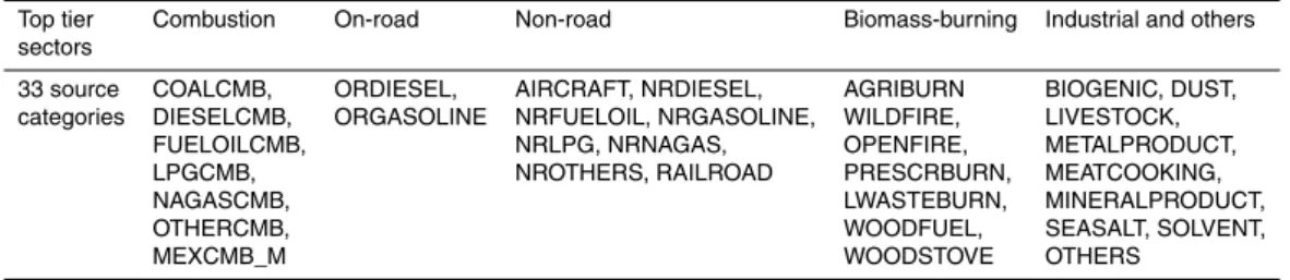
from the SPECIATE program (Simon et al., 2010). The component historically called “unidentified” in the emissions modeling process, is called “other” here because this portion of PM_2.5 is derived from measurements that provide the composition of the emissions, and includes element species which can be used to track source specific impacts on primary PM2.5. We group the emissions into 33 integrated source

cate-25

(8)

ACPD

13, 26657–26698, 2013

apportionment

Y. Hu et al.

Title Page

Tables Figures

◭ ◮

Back Close

Full Screen / Esc

Discussion

P

a

per

|

D

iscussion

P

a

per

|

Discussion

P

a

per

|

Discuss

ion

P

a

per

|

We apply the above modeling system to simulate PM2.5and gaseous concentrations for the month of January 2004, with 1–3 January as ramp-up days. The simulations of major PM2.5 and gaseous species were compared against measurements from multi-ple monitoring networks (Table S3) with performance statistics well within the normal range of current state-of-the-art CTM’s (Boylan and Russell, 2006; Tesche et al., 2006).

5

We also computed DDM-3D/PM first-order sensitivity coefficients for each source ex-cept SEASALT, as well as boundary and initial conditions (the sensitivity parameters are defined as the summation of all emitted compounds). The sensitivity coefficients of boundary and initial conditions were found minimal and therefore ignored in our cal-culations. For SEASALT we directly used the simulated concentrations of Na+ and Cl−

10

from sea salt emissions in the model, as sensitivities of Na+ or Cl− to SEASALT emis-sions. Sensitivities of other species (including other elements, ions and total mass of PM2.5) to SEASALT emissions were derived by applying the composition profile (Table S4) for each species relative to the Na+sensitivities. For the other 32 sources, element (metals and minerals) sensitivity coefficients that are not explicitly simulated by CMAQ

15

are derived by applying composition profiles (Table S4) for those elements relative to the modeled, source specific, “other” PM_2.5sensitivities, respectively. The source com-position profiles of all the 33 categories are assembled from the 86 profiles examined in Reffet al. (2009) by emissions-weighted averaging of corresponding member profiles (determined by SCC groupings). 24 h average simulated PM2.5 species, including

de-20

rived elements’ concentrations, are paired with 24 h average measurements at Chem-ical Speciation Network (CSN) sites (Fig. 1) for further use in optimization. We use 35 elements in PM2.5that are measured at each CSN site along with major components and total mass (Table S5). Detection limit and measurement uncertainty were used to screen for measurements that are invalid or below the detection limit (DL). Values below

25

DL were set to one half of the detection limit and the uncertainty was set to 2/3 of the DL (Marmur et al., 2006). Organic and elemental carbon measurements were artifact corrected and converted from thermal optical transmittance (TOT) values to thermal op-tical reflectance (TOR) equivalents using the method (Malm et al., 2011) recommended

(9)

ACPD

13, 26657–26698, 2013

apportionment

Y. Hu et al.

Title Page

Tables Figures

◭ ◮

Back Close

Full Screen / Esc

Discussion

P

a

per

|

D

iscussion

P

a

per

|

Discussion

P

a

per

|

Discuss

ion

P

a

per

|

by US EPA (http://www.epa.gov/ttn/naaqs/standards/pm/data/20120614Frank.pdf; see Note S1).

2.2 CTM source apportionment

Source impacts (and initial and boundary condition impacts) can be estimated using a Taylor series approach (Cohan et al., 2005):

5

SACTM_i_,_j =

K

X

k=1



Pj,k

∂c_i ∂pj,k

+P 2

j,k

2

∂2c_i ∂p2_j_,_k +

L

X

l=1;l6₌k

Pj,kPj,l

2

∂2c_i ∂pj,k∂pj,l



+HOT (3)

where SACTM_i_,_j is the CTM simulated impact (source apportionment result) of source

j(j=1, . . .JCTM, with JCTM being the total number of sources that are included in the CTM simulation, treating initial and boundary conditions as “sources”) on PM2.5species

i (i=1, . . .N with N being the total number of such species) at the receptor; P_j_,_k is

10

either the emission rate of compoundk (k =1, . . . ,K) (k can be different thani, ac-counting for species transformations) from sourcej, i.e.Ej,k, or the initial or boundary

concentration of compoundk;l andLare the same ask andK;p_j_,_k(p_j_,_l) is the sensi-tivity parameter forPj,k(Pj,l), and HOT stands for high order terms. The total impact of

sourcej on the PM2.5concentration using CTM method (SR CTM

j ) is found by summing

15

its impact on each species concentration:

SR_jCTM=

N

X

i=1

SACTM_i_,_j (4)

(10)

ACPD

13, 26657–26698, 2013

apportionment

Y. Hu et al.

Title Page

Tables Figures

◭ ◮

Back Close

Full Screen / Esc

Discussion

P

a

per

|

D

iscussion

P

a

per

|

Discussion

P

a

per

|

Discuss

ion

P

a

per

|

significant transformation, so

SACTM_i_,_j ≈

K

X

k₌1

Pj,k

∂ci

∂pj,k

=

K

X

k₌1

S_i(1)_,_j_,_k =S(1)_i_,_j (5)

whereS(1)_i_,_j_,_k is the semi-normalized first-order sensitivity of speciesi’s concentration to emission rate (or initial and boundary conditions) of compoundk from sourcej, while

S_i(1)_,_j is the similar first-order sensitivity to the emissions of all compounds from sourcej,

5

here as computed by CMAQ with DDM-3D/PM. Again, the notations for time and space dependencies are dropped for simplicity.

This result can be compared with the CMB method, which is based on apportioning each species proportional to the relative amount of that species in the PM_2.5emissions from a source:

10

SACMB_i_,_j =Ej,i

Ej

SRCMB_j =fi,jSR_jCMB (6)

Wherefi,j= E_j_,_i

E_j represents the original source profile used by CMB, i.e. the emission

fraction of species i(E_j_,_i) of the total PM_2.5 (E_j) emitted from source j (j₌1, . . .JCMB

withJCMBbeing the total number of emission sources that the CMB approach consid-ers, sourcej here can be different than the sources CTM includes) and SR_jCMB is the

15

CMB-calculated impact of sourcej on total PM2.5 concentration. One can extend the definition off_i_,_j for CTMs using Eq. (5) that includes the source impacts on condensed secondary pollutants in the analysis. Hence, an effectivef_i∗_,_j is found as:

f_i∗_,_j= SA CTM

i,j

SRCTM_j = S(1)_i_,_j

N

P

i=1

S_i(1)_,_j

=

K

P

k₌1

S(1)_i_,_j_,_k

N

P

i=1

K

P

k=1

S_i(1)_,_j_,_k

(7)

(11)

ACPD

13, 26657–26698, 2013

apportionment

Y. Hu et al.

Title Page

Tables Figures

◭ ◮

Back Close

Full Screen / Esc

Discussion

P

a

per

|

D

iscussion

P

a

per

|

Discussion

P

a

per

|

Discuss

ion

P

a

per

|

Equation (7) reveals that when there are no emissions of PM_2.5 component i from source j, f_i∗_,_j can still be non-zero, as the source could still contribute to secondary production of PM2.5.

2.3 CTM-CMB hybrid source apportionment approach

At monitoring locations, on days with sufficient PM_2.5composition measurements

avail-5

able, the following species balance equations can be built for a CMB solution:

c_iobs=

JCMB

X

j=1

fi,jSR_jCMB+e_iCMB (8)

wherec_iobs is the measured concentration for theith PM2.5 species, ande CMB

i is the

concentration prediction error to be minimized. CMB solves the species balance equa-tions to calculate a set ofSR_jCMBusing fixed source profilesfi,j (with uncertainties) that

10

minimizes the weighted squared error in the simulated concentrations (Watson, 1984). Likewise, similar species balance equations can be built at the same receptors using the initial source apportionments from CMAQ DDM-3D/PM results as follows:

c_iobs=

JCTM

X

j=1

SACTM_i_,_j +eCTM_i =

JCTM

X

j=1

K

X

k=1

S_i(1)_,_j_,_k+eCTM_i =

JCTM

X

j=1

S(1)_i_,_j +eCTM_i (9)

The extension to using CTM results is shown in the second through the fourth equalities

15

(12)

ACPD

13, 26657–26698, 2013

apportionment

Y. Hu et al.

Title Page Abstract Introduction Conclusions References Tables Figures ◭ ◮ ◭ ◮ Back Close

Full Screen / Esc

Printer-friendly Version Interactive Discussion Discussion P a per | D iscussion P a per | Discussion P a per | Discuss ion P a per |

Utilizing Eq. (9) we can evaluate the initial source apportionment results for a mea-surement at a receptor by calculating the square prediction error as:

χ2=

N

X

i₌1

       

cobs_i −

JCTM

P

j=1

SACTM_i_,_j !2

σ2

cobs_i

        (10)

whereσ_Cobs

i is the uncertainty in the measured concentration of speciesiobtained from the CSN measurement uncertainty.

5

Equation (10) also sheds light on an opportunity to further minimize the CTM’s pre-diction error in a least square solution that mimics the CMB method. This leads to a new method of conducting source apportionment in a SM-RM hybrid approach. One way to achieve this is to calculate a new set ofSR_jCTM using the extended f_i∗_,_j that minimizes the weighted squared error in the simulated concentrations as follows:

10

χ2=

N

X

i=1

       

cobs_i −

JCTM

P

j₌1

f_i∗_,_jSR_jCTM !2 σ2 cobs i         (11)

While this approach is similar to CMB, it accounts for secondary contributions and other atmospheric processing using the extendedf_i∗_,_j. If Eq. (11), alone, were used to develop revised source impacts, it would not fully take into account the information provided by the CTM about the estimated size and location of various emission sources and their

15

probable impact on pollutant concentrations at a receptor, i.e., the initial source impact

(13)

ACPD

13, 26657–26698, 2013

apportionment

Y. Hu et al.

Title Page

Tables Figures

◭ ◮

Back Close

Full Screen / Esc

Discussion

P

a

per

|

D

iscussion

P

a

per

|

Discussion

P

a

per

|

Discuss

ion

P

a

per

|

estimatesSR_jCTM=

N

P

i=1

SACTM_i_,_j . As formulated in Eq. (11), this information is only used in the calculation of f_i∗_,_j, but the magnitudes of the source impacts are lost. Further, collinearity and uniqueness issues, such as different sources sharing similar source profiles, would still impact the solution of the system of equations.

Instead of the above approach, the CMB concept is extended to directly use the

5

initial estimates ofSACTM_i_,_j as well as the initial simulated concentrationsc_iinit from the CTM to refine the estimated source impacts. Defining Rj as a scale factor applied to

the initial estimate of impact of sourcej(or initial or boundary conditions), SArefnd_i_,_j , the refined CTM-simulated impact of sourcej on speciesi is obtained as:

SArefnd_i_,_j =RjSAinit_i_,_j (12)

10

Here SAinit_i_,_j is the initial source impact (SA_iinit_,_j is the same as previous SACTM_i_,_j and is used from now on to distinguish fromSArefnd_i_,_j ). As such, refinements to source impacts can be found in a similar fashion to traditional CMB approaches by solving forRj to

minimizeχ2, where:

χ2=

N

X

i=1

c_iobs−c_iinit−

JCTM

P

j=1

(Rj−1)SA

init

i,j

!2

σ2

c_iobs

(13)

15

However, without further constraintsRj can be physically unrealistic and would not

(14)

ACPD

13, 26657–26698, 2013

apportionment

Y. Hu et al.

Title Page

Tables Figures

◭ ◮

Back Close

Full Screen / Esc

Discussion

P

a

per

|

D

iscussion

P

a

per

|

Discussion

P

a

per

|

Discuss

ion

P

a

per

|

Rj:

χ2 =

N

X

i=1



      

cobs_i −cinit_i −

JCTM

P

j=1

(Rj−1)SA

init

i,j

!2

σ2

c_iobs+σ

2

SRCTM_i



      

+ Γ

JCTM

X

j=1 (lnRj)

σ_ln2_R

j 2

(14)

whereσ_SRCTM

i is the a priori uncertainty in CTM-derived total sources’ impact on the

ith species, which is added to give weight for initial source impact estimates for dif-ferent species and represents model errors. One can estimateσ_SRCTM

i as proportional

5

to observed concentrationσ_SRCTM

i =δi∗c obs

i , with δi as normalized model errors. The

second term of the equation accounts for uncertainties in the CTM-derived individual source impacts due to emissions error.σlnR_j is the a priori uncertainty of the natural

log of sourcej’s scale factor. The logarithmic form is used as it has the same value on a relative basis. This naturally constrainsR_j to be positive._Γ is introduced to balance

10

the two terms in Eq. (14).

The objective function expressed as Eq. (14) can be minimized by using various optimization algorithms available for nonlinear optimization problems with constraints. We have tested a few such algorithms, including the algorithm of Sequential Least-Square Quadratic Programming (SLSQP) (Kraft, 1988, 1994) and L-BFGS, a

limited-15

memory quasi-Newton optimization function (Liu and Nocedal, 1989; Nocedal, 1980). With both the SLSQP and L-BFGS methods one can set lower and upper limits on

Rj for each individual source. We chose L-BFGS for our demonstration case study.

As R_j is optimized, the refined estimates of individual source impacts by species at a specific location are then given by Eq. (12). The level of remaining error in the refined

20

concentration predictions can be found using Eq. (13).

(15)

ACPD

13, 26657–26698, 2013

apportionment

Y. Hu et al.

Title Page

Tables Figures

◭ ◮

Back Close

Full Screen / Esc

Discussion

P

a

per

|

D

iscussion

P

a

per

|

Discussion

P

a

per

|

Discuss

ion

P

a

per

|

2.4 Application and case study

The hybrid method was applied for January of 2004 to calculate PM2.5 source impact scale factors at 164 CSN monitors for which we had valid speciated PM2.5 data. By using the valid measurements at each of these CSN sites for each valid day, the initial source impacts were evaluated through Eq. (14) to obtain impact scale factors and

re-5

fined source impacts estimates. The L-BFGS algorithm was used with box constraints that limitedR_j to be between 0.1 and 10.0 (different sets of limits have been tested, up to the range of between 0.02 and 50.0). Two steps were used to apply L-BFGS to find the final optimizedRj. First, an initial choice forΓwas set asΓ =_JCTMN =

41

33=1.24

to equally weigh the two terms in the objective function and obtain the initial optimal

10

Rj. Then, the initial optimal Rj were used to create a new Γ as the value of the first

term of the objective function divided byJCTM. The newΓ (typically about 20) is then applied to obtain the final optimizedRj. HereσlnR_j are determined by considering the

daily emission estimates uncertainties for each source (Table S2) derived from litera-ture (Hanna et al., 1998, 2001, 2005). In general, regulated sectors such as industrial,

15

on-road and non-road sources have lower uncertainties, non-regulated sectors such as residential related sources, dust and biomass-burning have much higher uncertain-ties. Because the refinements are applied daily, the uncertainties used account for the day-to-day variability in source strengths. For example, prescribed burning events can be quite variable in time. For traffic, day-specific emissions patterns are used, so the

20

source strength’s variability is smaller. Sources for which direct emissions monitoring is available are assigned the lowest uncertainty. To determine σ_SRCTM

i , δi (Table S6) are chosen as the typical normalized prediction errors of PM2.5 species as found in regional applications of state-of-the-art CTM models (Appel et al., 2008; Boylan and Russell, 2006; Tesche et al., 2006). Results were found not very sensitive to the range

25

of values ofσlnR_j andσSRCTM_i tested.

(16)

At-ACPD

13, 26657–26698, 2013

apportionment

Y. Hu et al.

Title Page

Tables Figures

◭ ◮

Back Close

Full Screen / Esc

Discussion

P

a

per

|

D

iscussion

P

a

per

|

Discussion

P

a

per

|

Discuss

ion

P

a

per

|

lanta, Chicago, Detroit, Los Angeles, New York, and Pittsburgh areas, representing urban/suburban locations across the country. Additional information for these six sites can be found in Tables S7 (basic site information) and Table S8 (emissions estimates surrounding each site). For comparison, we also conducted CMB modeling at the At-lanta site using the same measurement dataset and collected source apportionment

5

results from literature at the other five sites.

3 Results

3.1 Impact scale factors and refined concentration predictions

The hybrid method was applied to obtainR_j and to further refine the initial source im-pact estimates. AnRj of less than 1.0 means that the refined impact is reduced from

10

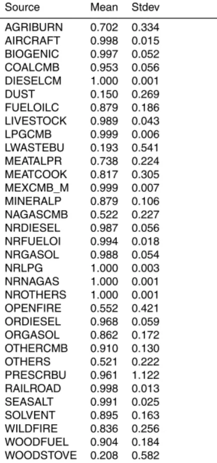
the original (suggesting that the emissions are biased high or that the CTM is leading to a high bias in the source-receptor relationship) while larger than 1.0 means that the im-pact is increased from the initial simulation. TheRj values obtained for the 33 sources

have means ranging from 0.15 to 1.0 with sources of higher uncertainties having larger standard deviations (Table 2). In general, sources that are commonly considered as

15

having high uncertainties were found to have Rj values deviating the most from 1.0,

while those sources considered less uncertain were found to haveRj values near 1.0.

This is expected, in part because of the second term in the weighting function. The scale factors are also found to be quite consistent (i.e. in same directions), in general, for the same source between locations and between days at the same location (Table

20

S9). Most significantly, R_j’s cumulative distribution functions are found to be distinc-tive between sources (Fig. S1). This is true even between biomass-burning sources although most of them have a similar composition in emissions (Fig. S1a). Dust, lawn waste burning (LWASTEBURN) and woodstove impacts (and other biomass-burning sources as well, although to a lesser extent) are found to be biased high (R_j values

25

typically ∼0.1). This is consistent with findings of prior studies (Baek, 2009; Chow

(17)

ACPD

13, 26657–26698, 2013

apportionment

Y. Hu et al.

Title Page

Tables Figures

◭ ◮

Back Close

Full Screen / Esc

Discussion

P

a

per

|

D

iscussion

P

a

per

|

Discussion

P

a

per

|

Discuss

ion

P

a

per

|

et al., 2007; Tian et al., 2009) that emission rates for these sources were overesti-mated. Also, prescribed burning impacts are found to be biased low (Rj values being

close to 10.0) a small portion of the time due to its high day-to-day variations. Typically, prescribed burn emissions are distributed uniformly over time in the inventories while in realty burns occur on days with favorable burning conditions. For most other sources

5

(Fig. S1b–d), impact scale factors are typically closer to 1.0, with most of theRjvalues

between 0.8 and 1.1, with the exceptions of metal processing, cooking processes, fuel oil and natural gas combustion, on-road gasoline vehicle and “others” sources. These six sources have more diverseRj values among locations and/or between days.

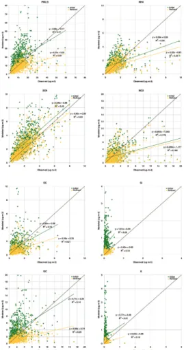
An indication of the magnitude of the refinements can be found by comparing the

10

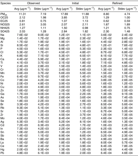
initial and refined individual species concentrations to the observations and can be quantified using the weighted least square error (i.e.χ2as expressed in Eq. 13). The simulated concentrations are found to be improved substantially compared to the initial simulation after refining source-impact estimates for major individual components and for most of the elements (Fig. 2 and Table 3). Note that several elements with very low

15

ambient concentrations (e.g. near the measurement uncertainty) were found to have slightly deteriorated agreement with observations (Table 3). However, results show that the refinedχ_{c, refnd}2 (Eq. 13 with obtainedRj), an overall index for remaining error, were

reduced by over 98 % on average (Fig. 3).

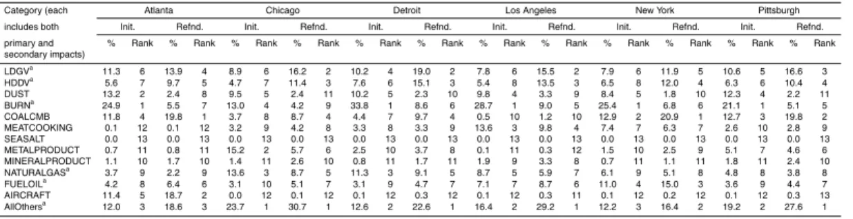
3.2 Initial and refined source impacts

20

Significant day-to-day variations are found in the initial source impact estimates (e.g. Table S10, as renormalized by total source impact), being more pronounced for some sources, such as power plants (i.e. coal combustion) and industrial sources. For exam-ple, in Atlanta, power plants (coal combustion) can contribute over 30 % on one day but only about 5 % on other days (primarily as secondary sulfates). In Chicago, metal

25

processing contributes 20 % on some days but less than 10 % on other days. On-road gasoline impact can also vary significantly day to day, such as in Detroit, it varies from

(18)

ACPD

13, 26657–26698, 2013

apportionment

Y. Hu et al.

Title Page

Tables Figures

◭ ◮

Back Close

Full Screen / Esc

Discussion

P

a

per

|

D

iscussion

P

a

per

|

Discussion

P

a

per

|

Discuss

ion

P

a

per

|

burns, contribute significantly on some days in Atlanta, but have virtually zero impact on other days.

Refined source impacts changed significantly from the initial estimates for sources with high uncertainties, such as woodstove and dust, as well as other biomass-burning sources, but changed much less or little for other sources (compare left and right

5

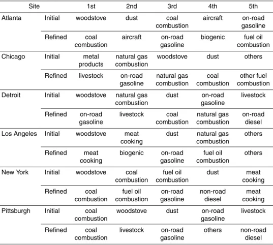
columns in Tables 4 and S10). Woodstove and dust were top ranked at all six sites from the initial estimates; however, refinement significantly lowered those sources’ im-pacts (Table 5). The differing adjustments between sources resulted in the rankings of top contributors changing. This indicates that estimates from SM-only methods might result in misleading source apportionment outcome due to the errors in emission

esti-10

mates on the specific day, as well as meteorological field and model parameter errors. For example, Marmur et al. (2006) found that the CMAQ-calculated impact of soil dust at Jefferson Street, Atlanta, GA (and other locations) was high when compared with two CMB estimates. This shows that it is necessary to evaluate SM source apportionment results using measurements.

15

The hybrid method can separate sources with similar composition, e.g., woodstove and prescribed burns, especially noting the di_fferent changes of these two sources be-tween their initial and refined impacts in Table S10a and d, as well as on-road and non-road diesel vehicles. This is because it starts from integrating estimated emis-sions from the inventory with source specific spatial and temporal resolution, instead

20

of starting from only the source composition like RMs do. In addition, with the hybrid method, secondary pollutants are apportioned to specific sources while in RMs they are aggregated together. For example, after the hybrid method refinement livestock impacts advance in rank among top contributors in Midwestern cities: Chicago, Detroit and Pittsburgh (Table 5), mostly through the secondary formation of ammonium and the

25

associated nitrate from NH₃emissions. Also, the two most common major contributors across the cities become coal combustion (except Los Angeles; Table 5), mainly due to the sulfate formation from SO2 emissions, and on-road gasoline vehicles, partially due to nitrate and organic matter formation from NO_xand VOC emissions.

(19)

ACPD

13, 26657–26698, 2013

apportionment

Y. Hu et al.

Title Page

Tables Figures

◭ ◮

Back Close

Full Screen / Esc

Discussion

P

a

per

|

D

iscussion

P

a

per

|

Discussion

P

a

per

|

Discuss

ion

P

a

per

|

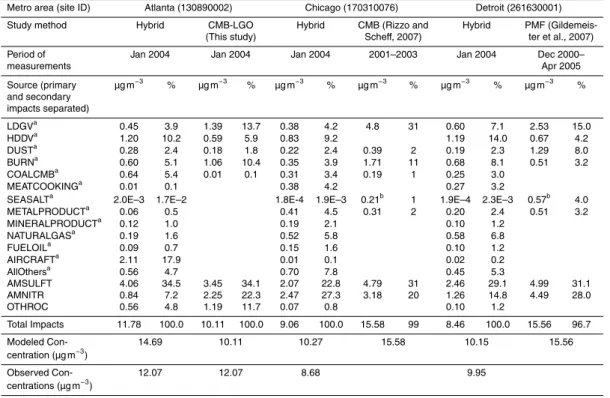
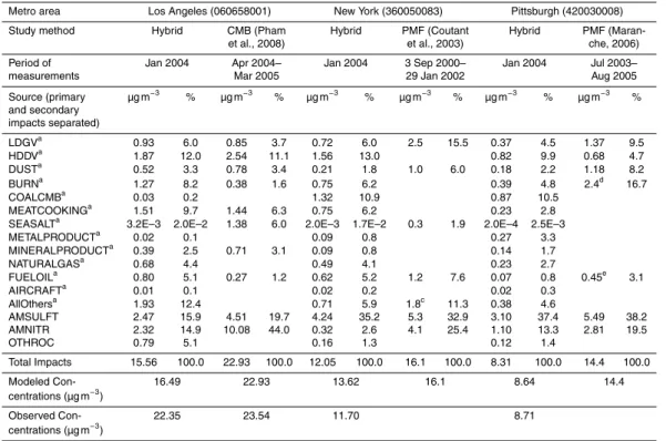
3.3 Comparison of refined source impacts with results from RM methods

In order to compare with other source apportionment studies, we first reduced the num-ber of sources from 33 to 13 by aggregating source impacts (Table 6). The 13 aggre-gated sources are chosen to cover the range of various sources in di_fferent locations as identified in prior studies. Sources having similar composition, e.g. various gasoline

5

and diesel vehicular sources, were merged accordingly. “AllOthers” included sources typically not resolved in traditional SA studies, e.g. livestock, biogenic and solvents as well as minor combustion and industrial sources. “AllOthers” (due to its large secondary contribution), and gasoline and diesel vehicles are top ranked in all six cities (Table 6). To make hybrid results directly comparable to that of RM methods, we further

sepa-10

rated the primary and secondary contributions in the aggregated source impacts and merged the secondary portions correspondingly into ammonium sulfates, ammonium nitrate, and secondary organic carbon (Details are discussed in Note S2). We compare the regrouped hybrid results to results of RM methods conducted at the same location by this or prior studies (Coutant et al., 2003; Gildemeister et al., 2007; Maranche, 2006;

15

Pham et al., 2008; Rizzo and Scheff, 2007) in Table 7. All the RM results were based on CSN measurements, though time periods for other RM results may differ (details of RM model applications are found in Note S3).

The hybrid approach resolved extra sources (with the total impacts of extra sources ranging between 20–30 % at the six sites) that are typically missing from RM results

20

(Table 7). This is consistent with∼20 % of the emissions that Baek (2009) found were not captured in most RM source apportionment applications. For example, CMB-LGO did not capture the aircraft source impact at the Atlanta site (Balachandran et al., 2012) as the profile is uncertain and similar to diesel combustion. However, measurement (Herndon et al., 2008; Lee et al., 2011) and modeling (Unal et al., 2005) studies have

25

(20)

ACPD

13, 26657–26698, 2013

apportionment

Y. Hu et al.

Title Page

Tables Figures

◭ ◮

Back Close

Full Screen / Esc

Discussion

P

a

per

|

D

iscussion

P

a

per

|

Discussion

P

a

per

|

Discuss

ion

P

a

per

|

RM methods using CSN data because their identification needs extra measurement information. For instance, CMB with particle-phase organic compounds as tracers us-ing measurements collected at the Jefferson street site has identified that natural gas combustion had a 1.1 % impact on PM_2.5in Atlanta (Zheng et al., 2002). Subramanian et al. (2007) used CMB with molecular markers and found that the impact of cooking

5

processes range from 1–5 % on PM2.5 concentrations in Pittsburgh. Compared to the hybrid results, the coal combustion primary impact estimates from RM methods are ei-ther missing or too low. This is because the trace element markers for coal combustion, Se and Sr, were not detected consistently in CSN samples due to low signal to noise ratios (Chen et al., 2010).

10

Hybrid results estimated total vehicle impacts (ranging between 14–22 %) were com-parable to the RM results found at the same urban/suburban locations, with an excep-tion in Chicago (Table S11). In Chicago, Rizzo and Scheff(2007) also conducted PMF modeling using the same composite data and their PMF results di_ffer from CMB results, e.g. for biomass burning (5 % vs. 11 %) and vehicle (23 % vs. 31 %) source impacts.

15

The PMF results were closer to the hybrid findings. At three of the four sites that the RM methods separated vehicle impacts between diesel and gasoline, the hybrid results do not agree with the RM methods on the diesel/gasoline split (Table S11): the hybrid method found higher impacts of diesel vs. gasoline (by a factor of 1.97–2.62), while the RMs found the opposite (0.28–0.49). The ratios of diesel/gasoline emissions

surround-20

ing the sites are in the range of 1.67–3.58 (Table S11). Subramanian at al. (2006) also found that diesel impacts in Pittsburgh tend to dominate by utilizing molecular markers. The split between diesel and gasoline vehicular impacts at Minnesota CSN sites from CMB solutions has been found to be inaccurate (Chen et al., 2011) when only regular measurements were used. Chow et al. (2007) suggested the difficulty of CMB to make

25

an accurate gasoline/diesel split without organic marker compounds.

Hybrid results tend to find lower secondary contributions than the RM methods, ex-cept in Chicago and Pittsburgh (Table S12). While the hybrid and RMs agree well on the ammonium sulfates at all six sites (16–37 % vs. 20–38 %; Table 7), the hybrid method

(21)

ACPD

13, 26657–26698, 2013

apportionment

Y. Hu et al.

Title Page

Tables Figures

◭ ◮

Back Close

Full Screen / Esc

Discussion

P

a

per

|

D

iscussion

P

a

per

|

Discussion

P

a

per

|

Discuss

ion

P

a

per

|

estimated lower secondary organic carbon (4.8 % vs. 11.7 %) in Atlanta, and they differ the most on secondary nitrate impacts (3–27 % vs. 20–44 %; Table 7). The difficulties in simulating particulate nitrate have been noted previously (Chang et al., 2011).

4 Discussion

The hybrid source apportionment method developed and applied here has been

5

demonstrated to be a novel way to improve SM-only CTM results by utilizing inde-pendent measurements. It also has advantages over RM methods. First, some limita-tions of RM methods are addressed (depending upon RM method): (1) the assumption that emissions are inert, with no chemical reactions, (2) not all source categories are considered, (3) potential collinearities between source compositions and, (4)

inconsis-10

tent or unrealistic results because receptor models do not include information on the strength and location of source emissions, and (5) not accounting for physical process such as complex meteorology. Second, the refinement and evaluation of the source impact estimates use measurement data that are independent from those used to de-velop the initial source impact estimates. Additionally, the hybrid method can be applied

15

to obtain spatial fields of source impacts providing hourly spatial fields.

A number of potential uncertainties from the CTM modeling can lead to uncertain-ties in the estimated impacts from the hybrid approach. The assumption for deriving concentrations and sensitivities for the elements that are not explicitly simulated in the CTM model might not hold always. The missing pathways of secondary organic

20

aerosol formation and inaccurate representation of nitrate formation in the CTM model can lead to underestimation of secondary source impacts. Errors in the meteorology may result in errors in the source fingerprints (f_i∗_,_j). Errors in the initial emissions inven-tory, particularly in the spatial and/or temporal variability and in the composition of the emissions, also introduce potential errors, particularly when using the model to

tem-25

(22)

ACPD

13, 26657–26698, 2013

apportionment

Y. Hu et al.

Title Page

Tables Figures

◭ ◮

Back Close

Full Screen / Esc

Discussion

P

a

per

|

D

iscussion

P

a

per

|

Discussion

P

a

per

|

Discuss

ion

P

a

per

|

the 24 h, speciated PM measurements. Thus, it is best to consider using results of this approach applied to 24 h averaged fields.

On the other hand, evaluating the hybrid model results on a species basis can help identify errors in the original source profiles. Additionally, including measurements from multiple sites in a region and/or spatially dense satellite retrievals in the process of

ad-5

justing emissions can further help stabilizeRj. This will provide more accurate

refine-ments and address the possibility of the measurerefine-ments taken at a single point being overly influenced by local sources. In this direction, the hybrid source results can be more accurate representations of the pollutant levels spatially because they integrate estimates of the spatial distribution of emissions and the local chemical and physical

10

atmospheric processes.

Supplementary material related to this article is available online at http://www.atmos-chem-phys-discuss.net/13/26657/2013/

acpd-13-26657-2013-supplement.pdf.

Acknowledgements. This publication was made possible by funding from the US EPA under 15

grants RD834799 and RD833866, NASA under grant NNX11AI55G and Georgia Power. Its contents are solely the responsibility of the grantee and do not necessarily represent the official views of the supporting agencies. Further, The US Government does not endorse the purchase of any commercial products or services mentioned in the publication.

References

20

Appel, K. W., Bhave, P. V., Gilliland, A. B., Sarwar, G., and Roselle, S. J.: Evaluation of the community multiscale air quality (CMAQ) model version 4.5: sensitivities impacting model performance; Part II – particulate matter, Atmos. Environ., 42, 6057–6066, 2008.

(23)

ACPD

13, 26657–26698, 2013

apportionment

Y. Hu et al.

Title Page

Tables Figures

◭ ◮

Back Close

Full Screen / Esc

Discussion

P

a

per

|

D

iscussion

P

a

per

|

Discussion

P

a

per

|

Discuss

ion

P

a

per

|

Baek, J.: Improving aerosol simulations: assessing and improving emissions and secondary organic aerosol formation in air quality modeling, Ph.D. Dissertation, Georgia Institute of Tecnology, Atlanta, GA, 140 pp., 2009.

Balachandran, S., Pachon, J. E., Hu, Y., Lee, D., Mulholland, J. A., and Russell, A. G.: Ensemble-trained source apportionment of fine particulate matter and method uncertainty 5

analysis, Atmos. Environ., 61, 387–394, 2012.

Binkowski, F. S. and Roselle, S. J.: Models-3 Community Multi-scale Air Quality (CMAQ) model aerosol component: 1. Model description, J. Geophys. Res., 108, 4183, doi:10.1029/2001JD001409, 2003.

Blanchard, C. L., Tanenbaum, S., and Hidy, G. M.: Source contributions to atmospheric gases 10

and particulate matter in the Southeastern united states, Environ. Sci. Technol., 46, 5479– 5488, 2012.

Boylan, J. W. and Russell, A. G.: PM and light extinction model performance metrics, goals, and criteria for three-dimensional air quality models, Atmos. Environ., 40, 4946–4959, 2006. Boylan, J. W., Odman, M. T., Wilkinson, J. G., Russell, A. G., Doty, K. G., Norris, W. B., and 15

McNider, R. T.: Development of a comprehensive, multiscale “one-atmosphere” modeling system: application to the Southern Appalachian Mountains, Atmos. Environ., 36, 3721– 3734, 2002.

Boylan, J. W., Odman, M. T., Wilkinson, J. G., and Russell, A. G.: Integrated assessment mod-eling of atmospheric pollutants in the Southern Appalachian Mountains: Part II – PM_2.5and 20

visibility, J. Air Waste Manage., 56, 12–22, 2006.

Bullock, K. R., Duvall, R. M., Norris, G. A., McDow, S. R., and Hays, M. D.: Evaluation of the CMB and PMF models using organic molecular markers in fine particulate matter collected during the Pittsburgh Air Quality Study, Atmos. Environ., 42, 6897–6904, 2008.

Burr, M. J. and Zhang, Y.: Source apportionment of fine particulate matter over the Eastern US 25

Part II: Source apportionment simulations using CAMx/PSAT and comparisons with CMAQ source sensitivity simulations, Atmos. Pollut. Res., 2, 318–336, doi:10.5094/APR.2011.5037, 2011a.

Burr, M. J. and Zhang, Y.: Source apportionment of fine particulate matter over the Eastern US Part I: Source sensitivity simulations using CMAQ with the Brute Force method, Atmos. 30

(24)

ACPD

13, 26657–26698, 2013

apportionment

Y. Hu et al.

Title Page

Tables Figures

◭ ◮

Back Close

Full Screen / Esc

Discussion

P

a

per

|

D

iscussion

P

a

per

|

Discussion

P

a

per

|

Discuss

ion

P

a

per

|

Byun, D. and Schere, K. L.: Review of the governing equations, computational algorithms, and other components of the Models-3 Community Multiscale Air Quality (CMAQ) modeling sys-tem, Appl. Mech. Rev., 59, 51–77, 2006.

Carter, W. P. L.: Documentation of the SAPRC-99 Chemical Mechanism for VOC Reactivity Assessment, Contract No. 92–329 and 95–308, California Air Resources Board, 2000. 5

CEP: Sparse Matrix Operator Kernel Emissions Modeling System (SMOKE) User Manual, Car-olina Environmental Program – The University of North CarCar-olina at Chapel Hill, Chapel Hill, NC, 2003.

Chang, W. L., Bhave, P. V., Brown, S. S., Riemer, N., Stutz, J., and Dabdub, D.: Heterogeneous atmospheric chemistry, ambient measurements, and model calculations of N₂O₅: a review, 10

Aerosol Sci. Tech., 45, 665–695, 2011.

Chen, L. W. A., Watson, J. G., Chow, J. C., DuBois, D. W., and Herschberger, L.: Chemical mass balance source apportionment for combined PM_2.5measurements from US non-urban and urban long-term networks, Atmos. Environ., 44(38), 4908–4918, 2010.

Chen, L. W. A., Watson, J. G., Chow, J. C., DuBois, D. W., and Herschberger, L.: PM_2.5source 15

apportionment: reconciling receptor models for US nonurban and urban long-term networks, J. Air Waste Manage., 61, 1204–1217, 2011.

Chow, J. C., Watson, J. G., Lowenthal, D. H., Solomon, P. A., Magliano, K. L., Ziman, S. D., and Richards, L. W.: PM₁₀ source apportionment in California San Joaquin Valley, Atmos. Environ. A, 26, 3335–3354, 1992.

20

Chow, J. C., Watson, J. G., Lowenthal, D. H., Chen, L. W. A., Zielinska, B., Mazzoleni, L. R., and Magliano, K. L.: Evaluation of organic markers for chemical mass balance source ap-portionment at the Fresno Supersite, Atmos. Chem. Phys., 7, 1741–1754, doi:10.5194/acp-7-1741-2007, 2007.

Cohan, D. S., Hakami, A., Hu, Y., and Russell, A. G.: Nonlinear response of ozone to emissions: 25

source apportionment and sensitivity analysis, Environ. Sci. Technol., 39, 6739–6748, 2005. Cooper, J. A. and Watson, J. G.: Reseptor oriented methods of air particulate source

appor-tionment, J. Air Pollut. Control Assoc., 30, 1116–1125, 1980.

Coutant, B. W., Holloman, C. H., Swinton, K. E., and Hafner, H. R.: Eight-site source apportion-ment of PM_2.5speciation trend data, EPA Contract No. 68-D-02-061, Work Assignment 1-05, 30

2003.

(25)

ACPD

13, 26657–26698, 2013

apportionment

Y. Hu et al.

Title Page

Tables Figures

◭ ◮

Back Close

Full Screen / Esc

Discussion

P

a

per

|

D

iscussion

P

a

per

|

Discussion

P

a

per

|

Discuss

ion

P

a

per

|

Dockery, D. W., Pope, C. A., Xu, X., Spengler, J. D., Ware, J. H., Fay, M. E., Ferris, B. G., and Speizer, F. E.: An association between air pollution and mortality in six US cities, The New Engl. J. Med., 329, 24, 1753–1759, 1993.

Doraiswamy, P., Davis, W. T., Miller, T. L., and Fu, J. S.: Source apportionment of fine particles in Tennessee using a source-oriented model, J. Air Waste Manage., 57, 407–419, 2007. 5

Dunker, A. M.: Efficient calculation of sensitivity coefficients for complex atmospheric models, Atmos. Environ., 15, 1155–1161, 1981.

Dunker, A. M.: The decoupled direct method for calculating sensitivity coefficients in chemical-kinetics, J. Chem. Phys., 81, 2385–2393, 1984.

Dunker, A. M., Yarwood, G., Ortmann, J. P., and Wilson, G. M.: Comparison of source appor-10

tionment and source sensitivity of ozone in a three-dimensional air quality model, Environ. Sci. Technol., 36, 2953–2964, 2002.

Emery, C., Tai, E., and Yarwood, G.: Enhanced Meteorological Modeling and Performance Eval-uation for two Texas Ozone Episodes, Prepared for the Texas Natural Resource Conservation Commissions, ENVIRON International Corporation, Novato, CA, 2001.

15

Gildemeister, A. E., Hopke, P. K., and Kim, E.: Sources of fine urban particulate matter in Detroit, MI, Chemosphere, 69, 1064–1074, 2007.

Grell, G., Dudhia, J., and Stauffer, D.: A Description of the Fifth-Generation Penn State/NCAR Mesoscale Model (MM5), NCAR/TN 398+STR, NCAR Technical Note: NCAR/TN-398+STR, 1994.

20

Hakami, A., Odman, M. T., and Russell, A. G.: Nonlinearity in atmospheric response: a direct sensitivity analysis approach, J. Geophys. Res.-Atmos., 109(D15), 2004.

Hanna, S., Chang, J., and Fernau, M.: Monte Carlo estimates of uncertainties in predictions by a photochemical grid model (UAM-IV) due to uncertainties in input variables, Atmos. Envi-ron., 32, 3619–3628, 1998.

25

Hanna, S. R. and Yang, R.: Evaluations of mesoscale models’ simulations of near-surface winds, temperature gradients, and mixing depths, J. Appl. Meteorol., 40, 1095–1104, 2001. Hanna, S. R., Lu, Z., Frey, H. C., Wheeler, N., Vukovich, J., Arumachalam, S., and Fernau, M. E.:

Uncertainties in predicted ozone concentration due to input uncertainties for the UAM-V photochemical grid model applied to the July 1995 OTAG domain, Atmos. Environ., 35, 891– 30

903, 2001.

(26)

ACPD

13, 26657–26698, 2013

apportionment

Y. Hu et al.

Title Page

Tables Figures

◭ ◮

Back Close

Full Screen / Esc

Discussion

P

a

per

|

D

iscussion

P

a

per

|

Discussion

P

a

per

|

Discuss

ion

P

a

per

|

transport model predictions, J. Geophys. Res., 110, D01302, doi:10.1029/02004JD004986, 2005.

Held, T., Ying, Q., Kleeman, M. J., Schauer, J. J., and Fraser, M. P.: A comparison of the UCD/CIT air quality model and the CMB source-receptor model for primary airborne partic-ulate matter, Atmos. Environ., 39, 2281–2297, 2005.

5

Henze, D. K., Seinfeld, J. H., and Shindell, D. T.: Inverse modeling and mapping US air quality influences of inorganic PM_2.5precursor emissions using the adjoint of GEOS-Chem, Atmos. Chem. Phys., 9, 5877–5903, doi:10.5194/acp-9-5877-2009, 2009.

Herndon, S. C., Jayne, J. T., Lobo, P., Onasch, T. B., Fleming, G., Hagen, D. E., Whitefield, P. D., and Miake-Lye, R. C.: Commercial aircraft engine emissions characterization of in-use air-10

craft at Hartsfield-Jackson Atlanta International Airport, Environ. Sci. Technol., 42, 1877– 1883, 2008.

Hu, Y., Odman, M. T., and Russell, A. G.: Mass conservation in the Community Multiscale Air Quality model, Atmos. Environ., 40, 1199–1204, 2006.

Kleeman, M. J., Ying, Q., Lu, J., Mysliwiec, M. J., Griffin, R. J., Chen, J. J., and Clegg, S.: 15

Source apportionment of secondary organic aerosol during a severe photochemical smog episode, Atmos. Environ., 41, 576–591, 2007.

Koo, B., Wilson, G. M., Morris, R. E., Dunker, A. M., and Yarwood, G.: Comparison of source apportionment and sensitivity analysis in a particulate matter air quality model, Environ. Sci. Technol., 43, 6669–6675, 2009.

20

Kraft, D.: A software package for sequential quadratic programming, Technical Report DFVLR-FB 88-28, Institut für Dynamik der Flugsysteme, Oberpfaffenhofen, July 1988.

Kraft, D.: Algorithm 733: TOMP – Fortran modules for optimal control calculations, ACM Trans. Math. Softw., 20, 262–281, 1994.

Laupsa, H., Denby, B., Larssen, S., and Schaug, J.: Source apportionment of particulate matter 25

(PM_2.5) in an urban area using dispersion, receptor and inverse modelling, Atmos. Environ., 43, 4733–4744, 2009.

Lee, B. H., Wood, E. C., Miake-Lye, R. C., Herndon, S. C., Munger, J. W., and Wofsy, S. C.: Reactive chemistry in aircraft exhaust implications for air quality, Transp. Res. Record, 2206, 19–23, 2011.

30

Lee, D., Balachandran, S., Pachon, J., Shankaran, R., Lee, S., Mulholland, J. A., and Rus-sell, A. G.: Ensemble-trained PM_2.5source apportionment approach for health studies, Env-iron. Sci. Technol., 43, 7023–7031, 2009.