A Reinforcement Learning for Train Marshaling Based on the Processing Time Considering Group Layout of Freight Cars

(1)

A Reinforcement Learning for Train Marshaling

Based on the Processing Time Considering Group

Layout of Freight Cars

Yoichi Hirashima

Abstract—In this paper a new method for generating mar-shaling plan of freight cars in a train is proposed. In the proposed method, marshaling plans based on the processing time can be obtained by a reinforcement learning system. In order to evaluate the processing time, the total transfer distance of a locomotive and the total movement counts of freight cars are simultaneously considered. Moreover, by grouping freight cars that have the same destination, candidates of the desired arrangement of the outbound train is extended. This feature is considered in the learning algorithm, so that the total processing time is reduced. Then, the order of movements of freight cars, the position for each removed car, the layout of groups in a train, the arrangement of cars in a group and the number of cars to be moved are simultaneously optimized to achieve minimization of the total processing time for obtaining the desired arrangement of freight cars for an outbound train. Initially, freight cars are located in a freight yard by the random layout, and they are moved and lined into a main track in a certain desired order in order to assemble an out bound train. Learning algorithm in the proposed method is based on the Q-Learning, and, after adequate autonomous learning, the optimum marshaling plan can be obtained by selecting a series of movements of freight cars that has the best evaluation.

Index Terms—Scheduling, Container Transfer Problem, Q-Learning, Freight train, Marshaling

I. INTRODUCTION

I

N recent years, logistics with freight train has important role in ecological aspects, because railway logistics is known to have smaller environmental load as compared to goods transportation with trucks ([1]). Train marshaling operation at freight yard is required to joint several rail transports, or different modes of transportation including rail. Transporting goods are carried in containers, each of which is loaded on a freight car. A freight train is consists of several freight cars, and each car has its own destination. Thus, the train driven by a locomotive travels several destinations disjointing corresponding freight cars at each freight station. In addition, since freight trains can transport goods only between railway stations, modal shifts are required for area that has no railway. In intermodal transports including rail, containers carried into the station are loaded on freight cars and located at the freight yard in the arriving order. The initial layout of freight cars is thus random. For efficient shift in assembling outbound train, freight cars must be rearranged before jointing to the freight train. In general, the rearrange-ment process is conducted in a freight yard that consists of a main-track and several sub-tracks. Freight cars are initially placed on sub tracks, rearranged, and lined into the main

Faculty of Information Science and Technology, Osaka Institute of Tech-nology, 1-79-1, Kita-yama, Hirakata City, Osaka, 573-0196, Japan. Tel/Fax: +86-72-866-5187 Email: [email protected]

track. This series of operation is called marshaling, and several methods to solve the marshaling problem have been proposed [2], [3]. Also, many similar problems are treated by mathematical programming and genetic algorithm[4], [5], [6], [7], and some analyses are conducted for computational complexities [7], [8]. However, these methods do not con-sider the processing time for each transfer movement of freight car that is moved by a locomotive.

(2)

In the learning algorithm, the state is defined by using a layout of freight cars, the car to be moved, the number of cars to be moved, and the destination of the removed car. An evaluation value called Q-value is assigned to each state, and the evaluation value is calculated by several update rules based on the Q-Learning algorithm. In the learning process, a Q-value in a certain update rule is referred from another update rule, in accordance with the state transition. Then, the Q-value is discounted according to the transfer distance of the locomotive. Consequently, Q-values at each state represent the total processing time of marshaling to achieve the best layout from the state. Moreover, in the proposed method, only referred Q-values are stored by using table look-up technique, and the table is dynamically constructed by binary tree in order to obtain the best solution with feasible memory space. In order to show effectiveness of the proposed method, computer simulations are conducted for several methods.

II. PROBLEM DESCRIPTION

The yard consist of 1 main track andmsub tracks. Define

kas the number of freight cars placed on the sub tracks, and

they are carried to the main track by the desirable order based on their destination. In the yard, a locomotive moves freight cars from sub track to sub track or from sub track to main track. The movement of freight cars from sub track to sub track is called removal, and the car-movement from sub track to main track is called rearrangement. For simplicity, the maximum number of freight cars that each sub track can have is assumed to be n, the ith car is recognized by an

unique symbol ci

(i=1;;k). Fig.1 shows the outline of

freight yard in the case k =30;m=n=6. In the figure,

L

c1

c2

c3

c4

c5

c6

c7

c8

c9

c10

c11

c12

c13

c14

c15

c16

c17

c18

c19

c25

c21

c22

c23

c24

c20 c26

c27

c28

c29

c30 [a]

[a]

[b] [b]

[c] [c]

[d] [d]

[e] [e]

[f] [f]

Tm [1] [2] [3] [4] [5] [6]

Fig. 1. Freight yard

track Tm denotes the main track, and other tracks [1], [2], [3], [4], [5], [6] are sub tracks. The main track is linked with sub tracks by a joint track, which is used for moving cars between sub tracks, or for moving them from a sub track to the main track. In the figure, freight cars are moved from sub tracks, and lined in the main track by the descending order, that is, rearrangement starts with c30and finishes with

c1. When the locomotive L moves a certain car, other cars

locating between the locomotive and the car to be moved must be removed to other sub tracks. This operation is called removal. Then, ifknm (n 1)is satisfied for keeping

adequate space to conduct removal process, every car can be rearranged to the main track.

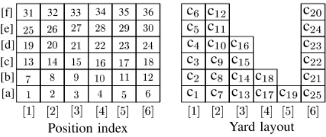
In each sub track, positions of cars are defined bynrows.

Every position has unique position number represented by

mn integers, and the position number for cars at main

track is 0. Fig.2 shows an example of position index for

k=30;m=n=6and the layout of cars for fig.1

1 2

3 4

5 6 7

8 9

10 11 12 13 14 15

16 17 18 19 20 21 22 23 24 25

26

27 28 29 30

[1℄

[1℄ [2℄ [3℄ [4℄ [5℄ [6℄ [2℄ [3℄ [4℄ [5℄ [6℄

Position index Yard layout c1

c2

c3

c4

c5

c7

c8

c9

c10

c11

c13

c14

c15

c16

c17

c18

c25

c21

c22

c23

c24

c19

[f] [e] [d] [c] [b] [a]

31 32 33 34 35 36 c6 c12 c 20

Fig. 2. Example of position index and yard state

In Fig.2, the position “[a][1]” that is located at row “[a]” in the sub track “[1]” has the position number 1, and the position “[f][6]” has the position number 36. For unified representation of layout of car in sub tracks, cars are placed from the row “[a]” in every track, and newly placed car is jointed with the adjacent freight car. In the figure, in order to rearrange c25, cars c24

;c 23

;c 22

;c

21 and c20 have to be

removed to other sub tracks. Then, sinceknm (n 1)

is satisfied, c25 can be moved even when all the other cars

are placed in sub tracks. In the freight yard, definex

i (1x

i

nm;i=1;;k)

as the position number of the car ci, and s=[x

1 ;;x

k ℄

as the state vector of the sub tracks. For example, in Fig.2, the state is represented by s = [1;7;13;19;25;31;

2;8;14;20;26;32;3;9;15;21;4;10;5;36;12;18;24;30;6;0;

0;0;0;0℄. A trial of the rearrange process starts with the

initial layout, rearranging freight cars according to the desirable layout in the main track, and finishs when all the cars are rearranged to the main track.

III. DESIRED LAYOUT IN THE MAIN TRACK In the main track, freight cars that have the same destina-tion are placed at the neighboring posidestina-tions. In this case, removal operations of these cars are not required at the destination regardless of layouts of these cars. In order to consider this feature in the desired layout in the main track, a group is organized by cars that have the same destination, and these cars can be placed at any positions in the group. Then, for each destination, make a corresponding group, and the order of groups lined in the main track is predetermined by destinations. This feature yields several desirable layouts in the main track.

Fig.3 depicts examples of desirable layouts of cars and the desired layout of groups in the main track. In the figure, freight cars c1,

, c

6 to the destination1 make group 1

, c7,

, c

18 to the destination2 make group 2

, c19, ,

c25 to the destination3 make group 3

, and c26, , c

30 to

the destination4 make group

4. Groups

1;2;3;4 are lined by

ascending order in the main track, which make a desirable layout. In the figure, examples of layout in group1are in the

dashed square.

Also, the layout of groups lined by the reverse order do not yield additional removal actions at the destination of each

(3)

c1

c6

...

.. .

c7

c18

c19

c25

c2

c3

c4

c5

group1

group2

group

3 4

(destination1)

(destination2)

(destination3)

4

desirable layouts for group1

Fig. 3. Example of groups

step1 step1

step1 step 2

step2 step2

step3 step3

step3

g1

g2

g

2

g2

g3

g4

g

4

g1:group1

g2:group2

g3:group3

g4:group4

Case (a) Case (b) Case (c)

L

L _L

L

Fig. 4. Group layouts

group. Thus, in the proposed method, the layout lined groups by the reverse order and the layout lined by decoupling order from both ends of the train are regarded as desired layouts. Fig.4 depicts examples of material handling operation for extended layout of groups at the destination of group1. In

the figure, step1 shows the layout of the incoming train. In case (a), cars in group1 are separated at the main track, and

moved to a sub-track by the locamotive L at step2. In cases (b),(c), cars in group1are carried in a sub-track, and group1

is separated at the sub-track. In the cases, group1 can be

located without any removal actions for cars in each group. Thus, these layouts of groups are regarded as candidate for desired one in the learning process of the proposed method.

IV. DIRECT REARRANGEMENT

When rearranging car that has no car to be removed on it is exist, its rearrangement precede any removals. In the case that several cars can be rearranged without a removal, rearrangements are repeated until all the candidates for rear-rangement requires at least one removal. If several candidates for rearrangement require no removal, the order of selection is random, because any orders satisfy the desirable layout of groups in the main track. In this case, the arrangement of cars in sub tracks obtained after rearrangements is unique, so that the movement counts of cars has no correlation with rearrangement orders of cars that require no removal. This operation is called direct rearrangement. When a car in a certain sub track can be rearrange directly to the main track

and when several cars located adjacent positions in the same sub track satisfy the layout of group in main track, they are jointed and applied direct rearrangement.

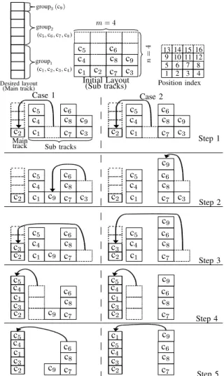
Fig.5 shows an example of arrangement in sub tracks existing candidates for rearranging cars that require no re-moval. At the top of figure, from the left side, a desired layout of cars and groups, the initial layout of cars in sub tracks, and the position index in sub tracks are depicted for

m=n=4;k=9. c 1

;c 2

;c 3

;c

4are in group 1

✁c 5

;c 6

;c 7

;c 8

are in group

2

, and group

1

must be rearranged first to the main track. In each group, any layouts of cars can be acceptable. In both cases, c2 in step 1 and c3 in step 3 are applied

the direct rearrangement. Also, in step 4, 3 cars c1 ;c

4 ;c

5

located ajacent positions are jointed and moved to the main track by a direct rearrangement operation. In addition, at step 5 in case 2, cars in group2and group3 are moved by a

direct rearrangement, since the positions of c7 ;c

8 ;c

6 ;c

9 are

satisfied the desired layout of groups in the main track. In case 1 of the example, the rearrangement order of cars that require no removal is c1

;c 2

;c 3

;c

4, and in case 2, the

order is c3 ;c

2 ;c

1 ;c

4. Although 2 cases have different orders

of rearrangement, the arrangements of cars in sub tracks and the numbers of movements of cars have no difference.

group1

group2

group

3 (c9)

Initial Layout (Sub tracks)

Case 1 Case 2

Step 1

Step 2

Step 3

Step 4

Step 5 Main

track Sub tracks

n

=

4

m=4

1 2 3 4 5 6 7 8 9 10 11 12 13 14 15 16

Position index

c1

c2

c3

c4

c5

c6

c6 c6

c6

c7

c9

c8 c8

c8

(c1

;c 2

;c 3

;c 4)

(c5

;c 6

;c 7

;c 8)

Desired layout (Main track)

Fig. 5. Direct rearrangements

V. REARRANGEMENT PROCESS

The rearrangement process for cars consists of following 6 operations :

(4)

(I) selection of a layout of groups in the main track, and rearrangement for all the cars that can apply the direct rearrangement into the main track, (II) selection of a freight car to be rearranged into the

main track,

(III) selection of a removal destinations of the cars in front of the car selected in (I),

(IV) selection of the number of cars to be moved, (V) removal of the cars to the selected sub-track, (VI) rearrangement of the selected car.

These operations are repeated until one of desirable layouts is achieved in the main track, and a series of operations from the initial state to the desirable layout is define as a trial.

Now, definehas the number of candidates of the desired

layout of groups. Each candidate in operation (I) is repre-sented by u

j 1

(1j 1

h).

In the operation (II), each group has the predetermined position in the main track. The car to be rearranged is defined as cT, and candidates of cT can be determined by excluding

freight cars that have already rearranged to the main track. These candidates must belong to the same group.

Also, defineras the number of groups✁g

las the number

of freight cars in groupl

(1lr), and u j

2

(h+1j 2

h+g l

)as candidates of c T.

In the operation (III), the removal destination of car located on the car to be rearranged is defined as cM. Then,

definingu j

3 (h+g

l

+1j

3

h+g

l

+m 1)as candidates of

cM, excluding the sub-track that has the car to be removed,

and the number of candidates is m 1.

In the operation (IV), definingpas the number of removal

cars required to rearrange cT, and defining

qas the number of

removal cars that can be located the sub-track selected in the operation (III), the candidate numbers of cars to be moved are determined byu

j4

;2mj 4

2m+minfp;qg 1.

In both cases of Fig.5, the direct rearrangement is con-ducted for c2 at step 1, and the selection of cT conducted

at step 2, candidates are u h+1

= [1℄;u h+2

= [4℄, that

is, sub-tracks where cars in group1 are located at the top.

u h+3

;u

h+4 are excluded from candidates. Then, u

h+2 =[4℄

is selected as cT. Candidates for the location of cT are

u h+5

=[1℄;u h+6

=[2℄;u h+7

=[3℄✁sub-tracks [1],[2], and

[3]. In case 1, u 6

= [2℄ is selected as c

M, and in case 2, u

h+7

= [3℄ is selected. After direct rearrangements of c 3

at step 3 and c1 ;c

4 ;c

5 at step 4, the marshaling process is

finished at step 5 in case 2, whereas case 1 requires one more step in order to finish the process. Therefore, the layout of cars and groups in the main track, the number of cars to be moved, the location the car to be rearranged and the order of rearrangement affect the total movement counts of freight cars.

VI. PROCESSING TIME FOR A MOVEMENT OF LOCOMOTIVE

A. Transfer distance of locomotive

When a locomotive transfer freight cars, the process of the unit transition is as follows: (E1). starts without freight cars, and reaches to the joint track, (E2) restart in reverse direction to the target car to be moved, (E3). joints them, (E4) pull out them to the joint track, (E5) restart in reverse direction, and transfers them to the indicated location, and

(E6) disjoints them from the locomotive. Then, the transfer distance of locomotive in (E1), (E2), (E4) and (E5) is defined as D

1, D

2, D

3 and D

4, respectively. Also, define the unit

distance of a movement for cars in each sub track asD min

v ✁

the length of joint track between adjacent sub tracks, or, sub track and main track as D

min

h. The location of the

locomotive at the end of above process is the start location of the next movement process of the selected car. Also, the initial position of the locomotive is located on the joint track nearest to the main track.

..

. Sub tracks

Main track

k

D

min

h

=

36

nDminh=6

(b) movement of cars

(a) position index

D minh

=1

D minh

=1

Dminv=1

mD

min

v

=

6

c1

c2

c3

c4

1 2 3 4 5 67 8 8

9 10 11 12 13 14 15 16

16

17 18 19 20 21 22 23 24 24

25 26 27 28 29 30 31 32 33 34 35 36

Fig. 6. Calculation of transfer distance

Fig.6 shows an example of transfer distance. In the figure,

m= n= 6; D minv

=D

minh

= 1;k =18, (a) is position

index, and (b) depicts movements of locomotive and freight car. Also, the locomotive starts from position 8, the target

is located on the position 18, the destination of the target

is 4, and the number of cars to be moved is 2. Since the

locomotive moves without freight cars from 8 to 24, the

transfer distance is D 1

+D

2

= 12 (D

1

= 5;D 2

= 7),

whereas it moves from24to16with 2 freight cars, and the

transfer distance isD 3

+D 4

=13(D 3

=7;D 4

=6).

B. Processing time for the unit transition

In the process of the unit transition, the each time for (E3) and (E6) is assumed to be the constant tE.

The processing times for elements (E1), (E2), (E4) and (E5) are determined by the transfer distance of the loco-motive D

i

(i=1;2;3;4), the weight of the freight cars W

moved in the process, and the performance of the locomo-tive. Then, the time each for (E1), (E2), (E4) and (E5) is assumed to be obtained by the function f(D

i

;W) derived

considering dynamics of the locomotive, limitation of the velocity, and control rules. Thus, the processing time for the unit transitiontUis calculated bytU=tE+

P 2 i=1

f(D i

;0)+ P

5 j=4

f(D j

;W). The maximum value oftUis define ast max

and is calculated by

t max

= tE+f(kD min

v

;0)+f(mD min

h ;0)

+f(mD min

h

+n;W)+f(kD minv

;W) (1)

VII. LEARNING ALGORITHM

Definehas the number of candidates of the desired layout

of groups. Each candidate is represented byu j1

(1u j1

Proceedings of the International MultiConference of Engineers and Computer Scientists 2012 Vol I,

(5)

h), and evaluated by Q 1

(u j1

). Then, Q 1

(u j1

) is updated

by the following equation when one of desired layout is achieved in the main track:

Q 1 (u j1 ) maxfQ 1 (u j1

);(1 )Q

1 (u

j1

)+

l

R g; (2)

where l denotes the total movement counts required to

achieve the desired layout✁is learning rate, is discount

factor, R is reward that is given only when one of desired

layout is achieved in the main track.

Define s(t) as the state at time t, rM as the sub track

selected as the destination for the removed car, pM as the

number of removed cars, q as the movement counts of

freight cars by direct rearrangement, and s 0

as the state that follows s. Also, Q

2 ;Q

3 ;Q

4 are defined as evaluation

values for(s 1

;u j

2 ),(s

2 ;u

j 3

),(s 3

;u j

4

), respectively, where s

1

= s ;s 2

= [s;c T

℄, s 3

= [s;c T

;rM℄ . Q 2 (s 1 ;u j 2 ), Q 3 (s 2 ;u j 3

)andQ 4 (s 3 ;u j 4

)are updated by following rules:

Q 2 (s 1 ;c T ) max uj 3 Q 3 (s 2 ;u j3 ); (3) Q 3 (s 2

;rM) max u j 4 Q 4 (s 3 ;u j 4 ); (4) Q 4 (s 3

;pM) (5)

8 > > > < > > > : (1 )Q 4 (s 3

;pM)+[R+ q+1

V 1

℄

(next action is rearrangement)

(1 )Q

4 (s

3

;pM)+[R+V 2

℄

(next action is removal)

V 1 =max uj 1 Q 2 (s 0 1 ;u j2 ); V 2 =max u j 2 Q 3 (s 0 2 ;u j 3 )

where is the learning rate, R is the reward that is given

when one of desirable layout is achieved, and is the

discount factor that is used to reflect the processing time of the marshaling and calculated by the following equation.

=Æ t max tU t max

; 0< <1;0<Æ<1 (6)

Propagating Q-values by using eqs.(3)-(6), Q-values are discounted according to the processing time of marshaling. In other words, by selecting the removal destination that has the largest Q-value, the processing time of the marshaling can be reduced.

In the learning stages, each u j

(1 j h+2m+

minfps;p

dg 1)is selected by the soft-max action selection

method[10]. ProbabilityP for selection of each candidate is

calculated by

~ Q i

(s ;u j

i

) =

Q i

(s ;u j i ) min u Q i (s ;u

j i ) max u Q i (s;u ji ) min u Q i (s;u ji ) (7) P(s i ;u j i ) = exp( ~ Q i (s j i ;u j i )=) X u2u j i exp( ~ Q i (s i ;u)=) ; (8)

(i=1;2;3;4):

In the addressed problem, Q 1 ;Q 2 ;Q 3 ;Q

4 become smaller

when the number of discounts becomes larger. Then, for complex problems, the difference between probabilities in candidate selection remain small at the initial state and large at final state before achieving desired layout, even after repetitive learning. In this case, obtained evaluation does not contribute to selections in initial stage of marshaling process,

and search movements to reduce the transfer distance of lo-comotive is spoiled in final stage. To conquer this drawback,

Q 1 ;Q 2 ;Q 3 ;Q

4 are normalized by eq.(7), and the thermo

constant is switched from 1 to 2 ( 1 >

2) when the

following condition is satisfied:

[The count of Q i (s j i ;u j i

)℄>;

s.t. Q i (s ji ;u ji

)>0; (9)

0<[the number of candidates foru j

i ℄

where is the threshold to judge the progress of learning.

The proposed learning algorithm can be summarized as follows:

1) Initialize all the Q-values as 0

2) Determine the layout of the main track amongu j1.

3) Conduct direct rearrangements.

4) If no cars are in sub tracks, go to 10✁otherwise go to

5

5) a Determine c

T among the candidates by

roulette selection (probabilities are calculated by eq. (8)),

b

Put reward as R=0,

c

Update the corresponding Q 4

(s 3

;pM) by

eq.(5) d Stores 1 ;c T

6) a Determine rM(probability for the selection is

calculated by eq.(8)) b

Update correspondingQ 3

(s 2

;rM)by eq.(4),

c

stores 2

;rM

7) a Determine pM(probability for the selection is

calculated by eq.(8)) b

Update correspondingQ 4

(s 3

;pM)by eq.(5)

c

Stores 3

;pM

8) RemovepM cars and place atrM

9) Go to 3

10) Receive the reward R, update Q 1

(s 1

;c T

)by eq.(3)

VIII. COMPUTER SIMULATIONS

Computer simulations are conducted for m = 12;n =

6;k=36and learning performances of following 5 methods

are compared:

(A) proposed method that evaluates the processing time of the marshaling operation, considering the layout of groups,

(B) a method that evaluates the transfer distance of the locamotive considering the layout of groups[11], (C) a method that evaluates the number of movements

of freight cars, considering the layout of gruops[11] (D) a method that evaluates the processing time, with

single layout of groups.

The initial arrangement of cars in sub tracks is described in Fig.7. In this case, the rearrantement order of groups is group 1 ;group 2 , group 3 , group 4

. Cars c1 ;;c

9 are in

group1 ✁c

10, , c

18 are in group 2

✁c 19

; ;c

27 are in

group3 ✁and c

28 ;;c

36 are in group

4. Other parameters

are set as = 0:9; = 0:2;Æ = 0:9;R = 1:0; =

0:95; 1

=0:1; 2

=0:05. In method (C), the discount factor is assumed to be constant, and set as =0:9 instead of

calculationg by eq.(6).

The locomotive assumed to accerarate and deaccerarate the train with the constant force10010

3

(6)

TABLE I

TOTAL PROCESSING TIME

processing time (sec.) methos best average worst method (A) 5328.06 5376.33 5407.88 method (B) 5331.81 5390.69 5423.99 method (C) 5337.18 5366.46 5416.54 method (D) 5688.26 5763.90 5839.88

10 3

kg in weight. Also, all the freight cars have the same weight,1010

3

kg. The locomotive and freight cars assumed to have the same length, and D

minv

=D

minh

=20m. The

velocity of the locomotive is limited to no more than 10m/s. Then, the locomotive accerarates the train until the velocity arrives 10m/s, keeps the velocity, and deaccerarates until the train stops within the indicated distance. When the velocity does not arrive 10m/s at the half way point, the locomotive starts to deaccerarate immediately. Then,t

max =462.

Fig.8 show the results. In Fig.8, horizontal axis expresses the number of trials and the vertical axis expresses the minimum prcessing time to achieve a desirable layout found in the past trials. Each result is averaged over 20 inde-pendent simulations. In Fig.8, the learning performance of method (A) is better than that of method (D), because solutions derived by method (A) uses the extended layout of groups effectively for reducing the total processing time. In method (C), the learning algorithm evaluates the number of movements of freight cars, and is not effective to reduce the total processing time. In method (B), only the total transfer distance of locamotive is evaluated, so that the total processing time is not improved adequately even if many trials are repeated. Total transfer distances of the locomotive at1:510

6

th trial are described in table.I for each method. Fig.9 shows final arrangements of freight cars generated by the best solutions derived by methods (A) and (D). Since the layout of group is extended, method (A) learns the layout of groups in order to reduce the total processing time, whereas the layout is fixed to the ascending order in method (D).

c1

c2

c3

c4 c5

c6 c7

c8

c9

c10

c11

c12

c13 c

14

c15

c16

c17

c18

c19

c20

c21

c22

c23

c24

c25

c26

c27

c28 c

29

c30

c31

c32

c33

c34

c35

c36 1

2

3

4

Fig. 7. Initial layout

IX. CONCLUSIONS

A new scheduling method has been proposed in order to rearrange and line cars in the desirable order onto the main track. The learning algorithm of the proposed method is derived based on the reinforcement learning, considering the total processing time of marshaling. In order to reduce the total processing time of marshaling, the proposed method learns the layout of groups, as well as the arrangement of freight cars in each group, the rearrangement order of cars, the number of cars to be moved and the removal destination of cars, simultaneously. In computer simulations, learning performance of the proposed method has been improved by using normalized evaluation and switching thermo constants in accordance with the progress of learning.

7000

6500

6000

5500

5000

0 2 4 6 8 10

10 4

M

in

im

u

m

p

ro

ce

ss

in

g

ti

m

e

(s

ec

.)

Trials (A)

(B)

(C) (D)

Fig. 8. Comparison of learning performances

c1

c2

c3

c4

c5

c6

c6 c 7

c7

c8

c9

c10

c11

c12

c13

c13 c

14

c14

c15

c16

c17

c18

c19

c20

c21

c22

c22 c

23

c23

c24

c25

c26

c27

c28

c29

c30

c31

c32

c33

c34

c35

c36

group

1

group1 group

2

group

2 group

3

group3 group

4

group

4

Head

Head Tail Tail

(A) (D)

Fig. 9. Final layouts

REFERENCES

[1] G. LI, M. MUTO, N. AIHARA, and T. TSUJIMURA, “Environmental load reduction due to modal shift resulting from improvements to railway freight stations,” Quarterly Report of RTRI, vol. 48, no. 4, pp. 207–214, 2007.

[2] U. Blasum, M. R. Bussieck, W. Hochst¨attler, C. Moll, H.-H. Scheel, and T. Winter, “Scheduling trams in the morning,” Mathematical Methods of Operations Research, vol. 49, no. 1, pp. 137–148, 2000. [3] R. Jacob, P. Marton, J. Maue, and M. Nunkesser, “Multistage methods

for freight train classification,” in Proceedings of 7th Workshop on Algorithmic Approaches for Transportation Modeling, Optimization, and Systems, 2007, pp. 158–174.

[4] L. Kroon, R. Lentink, and A. Schrijver, “Shunting of passenger train units: an integrated approach,” Transportation Science, vol. 42, pp. 436–449, 2008.

[5] N. TOMII and Z. L. Jian, “Depot shunting scheduling with combining genetic algorithm and pert,” in Proceedings of 7th International Conference on Computer Aided Design, Manufacture and Operation in the Railway and Other Advanced Mass Transit Systems, 2000, pp. 437–446.

[6] S. He, R. Song, and S. Chaudhry, “Fuzzy dispatching model and genetic algorithms for railyards operations,” European Journal of Operational Research, vol. 124, no. 2, pp. 307–331, 2000.

[7] E. Dahlhaus, F. Manne, M. Miller, and J. Ryan, “Algorithms for combinatorial problems related to train marshalling,” inProceedings of the 11th Australasian Workshop on Combinatorial algorithms, 2000, pp. 7–16.

[8] C. Eggermont, C. A. J. Hurkens, M. Modelski, and G. J. Woeginger, “The hardness of train rearrangements,”Operations Research Letters, vol. 37, pp. 80–82, 2009.

[9] C. J. C. H. Watkins and P. Dayan, “Q-learning,”Machine Learning, vol. 8, pp. 279–292, 1992.

[10] R. Sutton and A. Barto,Reinforcement Learning. MIT Press, 1999. [11] Y. Hirashima, “A new reinforcement learning method for train mar-shaling based on the transfer distance of locomotive,”Lecture Notes in Engineering and Computer Science: Proceedings of The International MultiConference of Engineers and Computer Scientists 2011, IMECS 2011, pp. 80–85, 2011.