A stochastic nonlinear oscillator model for glacial millennial-scale climate transitions derived from ice-core data

www.nonlin-processes-geophys.net/19/595/2012/ doi:10.5194/npg-19-595-2012

© Author(s) 2012. CC Attribution 3.0 License.

Nonlinear Processes

in Geophysics

A stochastic nonlinear oscillator model for glacial millennial-scale

climate transitions derived from ice-core data

F. Kwasniok1and G. Lohmann2

1_{College of Engineering, Mathematics and Physical Sciences, University of Exeter, Exeter, UK} 2_{Alfred Wegener Institute for Polar and Marine Research, Bremerhaven, Germany}

Correspondence to:F. Kwasniok (f.kwasniok@exeter.ac.uk)

Received: 16 May 2012 – Revised: 5 October 2012 – Accepted: 16 October 2012 – Published: 7 November 2012

Abstract. A stochastic Duffing-type oscillator model, i.e noise-driven motion with inertia in a potential landscape, is considered for glacial millennial-scale climate transitions. The potential and noise parameters are estimated from a Greenland ice-core record using a nonlinear Kalman filter. For the period from 60 to 20 ky before present, a bistable potential with a deep well corresponding to a cold stadial state and a shallow well corresponding to a warm intersta-dial state is found. The system is in the strongly dissipative regime and can be very well approximated by an effective one-dimensional Langevin equation.

1 Introduction

Past and future abrupt climate changes have been extensively discussed in recent years (e.g. Alley et al., 2003). A par-ticular subject of investigation are the abrupt climate transi-tions between cold stadials and warm interstadials during the last glacial period, the so-called Dansgaard-Oeschger (DO) events (Dansgaard et al., 1993). Their origin and dynami-cal mechanism is still controversial; it is not obvious which part of the Earth’s climate system is responsible for abrupt changes. DO events may be attributed to a temporary col-lapse and resumption of the Atlantic meridional overturn-ing circulation (Ganopolski and Rahmstorf, 2002). Other hy-potheses refer to internal oscillations in the climate system (Sakai and Peltier, 1997; Schulz et al., 2002; Timmermann et al., 2003) or external forcing mechanisms (Ganopolski and Rahmstorf, 2001; Braun et al., 2005).

Besides studies with complex numerical models, other have tried to reduce the system to low-order, box and con-ceptual models both in a deterministic and stochastic setting.

Different types of low-order models have been proposed to explain the dynamics of DO events. A bistable nonlinear sys-tem has been assumed in which shifts between the two dis-tinctly different states are triggered randomly by stochastic forcing (Ditlevsen, 1999; Ditlevsen et al., 2005; Kwasniok and Lohmann, 2009; Livina et al., 2010). Stochastic reso-nance (Benzi et al., 1982; Alley et al., 2001; Ganopolski and Rahmstorf, 2002) may or may not play a role in such a model. Recently, the mechanism of ghost stochastic resonance has been proposed (Braun et al., 2009) as a noise-induced phe-nomenon beyond classical stochastic resonance. Moreover, a system of nonlinearly coupled relaxation oscillators has been postulated (Schulz et al., 2002). Each of the oscillators rep-resents a fundamental climate mode with a characteristic fre-quency in the centennial-to-millennial band; nonlinear inter-action between the oscillators may lead to phase synchro-nisation and the development of a new climate mode with a joint frequency. Furthermore, a nonlinear thermal oscilla-tor has been proposed (Rial, 2004) where the timing of the deterministic external forcing is crucial for generating DO-like oscillations. In a conceptual model approach, Dima and Lohmann (2009) propose that millennial-scale variability can originate from rectification of an external forcing, and sug-gest that the thermohaline circulation, through a threshold response, could be the rectifier. The latter hypothesis is a combination of the externally driven and internal oscillation hypotheses.

of if the DO events can be characterised by a stochastic non-linear Duffing-type oscillator model.

2 Dynamical model

Abrupt palaeoclimatic changes are often assumed to be re-lated to a shift between two different stable states in a noise-driven nonlinear system (e.g. Alley et al., 2001; Ganopolski and Rahmstorf, 2002). A very simple conceptual model is stochastically driven motion in a one-dimensional potential landscape (e.g. Ditlevsen, 1999; Kwasniok and Lohmann, 2009). The governing equation is

˙

z= −U′(z)+τ η (1)

whereU (z) is a potential function, η is a white Gaussian noise with zero mean and unit variance andτ is the standard deviation of the stochastic forcing. The stationary probability density of the system is

p(z)∼exp

−2U (z) τ2

. (2)

We here extend the dynamical framework and adopt a two-dimensional model given by

˙

z=v+σ1η1 (3)

˙

v= −γ v−V′(z)+σ2η2 (4)

whereV (z)is a potential function andγis a dissipation con-stant.η1andη2are two independent Gaussian white noises with zero mean and unit variance;σ1 andσ2 are the stan-dard deviations of the noise forcings. The variablez corre-sponds to a palaeotemperature proxy as given by an ice-core record; the variablevis a velocity-like quantity (e.g. temper-ature change) which is here not explicitly specified further.

In the caseσ1=0, the system of Eqs. (3) and (4) is the well-known Kramers model for Brownian motion with iner-tia in a poteniner-tial (Kramers, 1940; Gardiner, 2010) with sta-tionary probability density:

p(z, v)∼exp −2γ σ₂2

V (z)+1

2v 2

!

. (5)

It is then equivalent to the second-order equation

¨

z+γz˙+V′(z)=σ2η. (6)

This is actually a nonlinear stochastic oscillator; for the particular choiceV (z)=1₄αz4+1₂βz2withα >0, it is the (noise-driven) Duffing oscillator which for β <0 exhibits bistability.

The stochastic terms are meant to account for model un-certainty and structural discrepancy between the model and the real system. Adding a noise term also in the equation for z (Eq. 3), which is uncommon, considerably enhances

the dynamical richness and realism of the model beyond the Kramers model. The system of Eqs. (3) and (4) forσ16=0 breaks the condition of detailed balance and therefore the time-reversal symmetry of the stationary joint probability density:p(z, v, t;z′, v′, t′)6=p(z′,−v′, t;z,−v, t′). It is ca-pable of producing temporally asymmetric time series; in fact, the characteristic saw-tooth shape is an important non-linear feature of DO events (Dansgaard et al., 1993). The sta-tionary probability densityp(z, v)is not straightforward any more, andzandvare no longer statistically independent. The one-dimensional potential model of Eq. (1) and the Kramers model are in detailed balance and are therefore not able to break the time-reversal symmetry.

In the limit of strong dissipation (Smoluchowski regime),

vcan be adiabatically eliminated from Eqs. (3) and (4) and the dynamics ofz well approximated by an effective one-dimensional Langevin equation given by Eq. (1) with

U (z)=V (z)/γ (7)

and

τ2=σ₁2+σ₂2/γ2. (8)

This can be shown by slightly extending standard results (Gardiner, 2010, Chap. 8.2).

The potentialV (z)is here assumed to be a general fourth-order polynomial (Kwasniok and Lohmann, 2009):

V (z)=a4z4+a3z3+a2z2+a1z (9)

with free parameters{ai}4i=1to be determined from data.

3 Model estimation

3.1 Unscented Kalman filter

The unscented Kalman filter (UKF) (Julier et al., 2000; Sitz et al., 2002; Julier and Uhlmann, 2004) is used for parame-ter estimation in the oscillator model. It allows for recursive estimation of unobserved states and parameters in stochastic nonlinear systems from incomplete, indirect and noisy obser-vations. The UKF keeps the full nonlinear system dynamics rather than linearising it but truncates the filter probability density to a Gaussian in each iteration by only propagating first and second moments.

We use the framework of a continuous-discrete nonlin-ear state space model. The evolution of the state vectorz= (z, v)T of dimensionn=2 is governed by the continuous-time, nonlinear stochastic dynamical system:

˙

z=f(z;λ)+ξ, (10)

ξ is a vector of Gaussian white noises with zero mean and covariance matrix:

Q=

σ₁2 0

0 σ₂2

. (11)

An augmented state vectorxof dimensionna=n+p=7 is formed by merging the state vector and the parameters. Equation (10), together with a constant dynamics for the pa-rameters

˙

λ=0, (12)

form the dynamical or state equation of the state space model:

˙

x=fa(x)+ξa. (13)

ξais the augmented noise process vector with corresponding covariance matrixQa. At discrete timestk, observationsykof

dimensionm=1 are available which are linked to the state by the observation equation:

yk=Hxk+εk. (14)

We here observe only the variablez; thus the observation op-erator isH=(1,0,0,0,0,0,0).εk is white Gaussian

obser-vational noise with mean zero and varianceR.

The UKF provides estimates of the system states and pa-rameters given a time series of noisy observations{yk}Nk=0. Letxˆk−1|k−1 be the mean estimate of the augmented state vector andPk−1|k−1its covariance matrix at time stepk−1 having processed all data up to time step k−1. The fil-ter density is represented by a small number of so-called sigma points that are propagated through the full nonlinear dynamical equations. The interval[tk−1, tk]is divided into

L equal subintervals of size h=(tk−tk−1)/L, and a se-quence of estimates{x_ˆl,Pl}Ll=0is generated. Having arrived atxˆl−1 andPl−1, we use 2na sigma points,{xi_l−1|l−1}

2na

i=1, each in augmented state space of dimension na, given as

{x_ˆl−1−wj_l−1,xˆl−1+wj_l−1}

na

j=1. The vectors{w

j l−1}

na

j=1 are the columns of A where A can be any matrix satisfying AAT=naPl−1. Here, we calculateAusing the Cholesky

de-composition ofPl−1. The sigma points are transformed as

xi_l|l−1=xi_l−1|l−1+hfa(xi_l−1|l−1), (15) and new mean and covariance estimates are given by

ˆ xl=

1 2na

2na X

i=1

xi_l|l−1 (16)

and

Pl=

1 2na

2na X

i=1

(xi_l|l−1−x_ˆl)(xil|l−1−xˆl)

T

+hQa. (17)

The sequence is initialised withxˆ0=xˆk−1|k−1andP0= Pk−1|k−1. We setxˆk|k−1=xˆLandPk|k−1=PL. Then the

es-timates of the states and the parameters as well as their un-certainties are updated using the new observation according to the Kalman update equations:

ˆ

xk|k =xˆk|k−1+Kkζk; (18)

Pk|k =(I−KkH)Pk|k−1. (19)

Here

ζk=yk−Hxˆk|k−1 (20)

is the innovation or residual,

Kk=Pk|k−1HTS_k−1 (21)

is the Kalman gain matrix and

Sk=HPk|k−1HT+R (22)

is the predicted residual covariance matrix. 3.2 Estimation of noise parameters

For estimation of the noise levelsσ1 andσ2, we follow the likelihood approach recently proposed by Kwasniok (2012). At time stepk, the predictive probability density of the UKF for the residualζkis a Gaussian with zero mean and variance

Sk. Thus the log-likelihood function of the data set is

l(σ1, σ2)= −

N

2 log 2π− 1 2

N

X

k=1

logSk+

ζ_k2 Sk

!

. (23)

The UKF is run for different noise parameters and the like-lihood maximised. It is sufficient to just calculate the likeli-hood on a fine enough mesh in noise parameter space and find the maximum. The method for estimating the noise lev-els is based on internal consistency; for the correct noise parameters, the uncertainty propagated by the Kalman filter matches the true predictive uncertainty reflected in the data.

4 Simulated data

We first use simulated data to test the ability of the method to reliably identify system parameters and noise levels. A symmetric double-well potential is chosen given byV (z)=

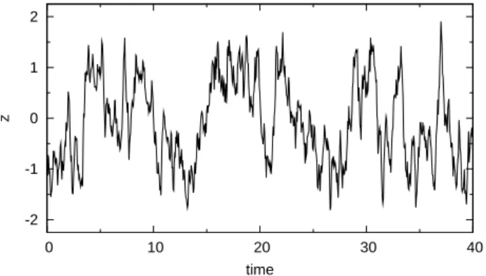
10z4−20z2. The damping constant isγ=10; the noise lev-els areσ1=1 andσ2=10. The system is integrated using the Euler-Maruyama scheme with a step size of 10−5. Only the variablezis observed. No observational noise is added. Figure 1 displays a sample trajectory of the variablezin the system. The time scale of transitions between the two stable states is of the same order as in the ice-core record consid-ered later (Fig. 4) when interpreting the system units as ky.

-2 -1 0 1 2

0 10 20 30 40

z

time

Fig. 1. Sample trajectory of z in the oscillator with symmetric double-well potential.

Letz∗=0 be the maximum of the potential. Introducing the

frequencyω∗byω2∗= |V′′(z∗)|we haveγ /ω∗≈1.6 which

is neither small nor large compared to 1, corresponding to an intermediate regime ofγ. One may also look at the be-haviour of the system in the vicinity of the minimaz0= ±1. We introduce the deviation from the equilibriumx=z−z0 and the frequencyω0byω₀2=V′′(z0). For small|x|, the de-terministic part of the system is then given by the damped harmonic oscillator equation:

¨

x+γx˙+ω₀2x=0. (24)

The solution type is characterised by the damping ratioρ=

γ

2ω0. The valuesρ=0, 0< ρ <1,ρ=1 andρ >1

corre-spond to the undamped, underdamped (oscillatory), critically damped and overdamped regimes, respectively. We here have

ρ≈0.56. The system exhibits damped oscillations with pe-riod 0.85 ande-folding time 0.2.

In order to have a comparison with the relatively short ice-core record, we use simulated time series of lengthN=

800 with sampling intervalδt=0.05, spanning a time pe-riod of 40 time units, and then perform multiple experi-ments. The UKF is initialised with the parameter setting

(a4, a3, a2, a1, γ )=(5,5,−10,5,5). The initial state esti-mate is given by the initial observation; the initial velocity estimate is set to zero. The initial variances are all set to 100 except for the state where it is zero as there is no ob-servational noise. The step size in the UKF ish=δt /100=

0.0005; we set R=10−12. The data set spanning a period of 40 time units with 800 data points is too small to obtain well-converged estimates for the parameters. Therefore, the data are processed 10 times to improve the estimates. Each new sweep is started with the final estimates for the parame-ters and uncertainties from the preceding sweep but the off-diagonal elements of the covariance matrix set to zero (Sitz et al., 2002).

Figure 2 shows the log-likelihood as a function of the noise levelsσ1andσ2for a particular realisation taken over the last sweep through the data. Using a grid of size 0.01 forσ1and

0.9

0.95 1

1.05 8 10

12 14

16 -20

-15 -10 -5

σ1

σ2

Fig. 2.Simulated data: Log-likelihood as a function of the noise levelsσ1andσ2. Neighbouring contours differ by a factor of 2 in

likelihood.

0.5 forσ2, the maximum of the likelihood is atσ1=0.99 and

σ2=11.5. Due to the shortness of the time series, estimation of the noise levels is quite ill-conditioned as the likelihood function is relatively flat.

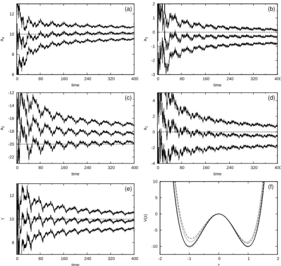
Figure 3 displays the parameter estimates together with the error standard deviations as the algorithm proceeds through the time series. Taking averages over the last sweep of 800 data points and the final error estimates, the values of the parameters are a4=10.10±0.59, a3= −0.30±0.48,

a2= −18.33±1.38,a1= −0.49±1.26 andγ=9.83±0.66. The uncertainties in the estimates are considerable as one ex-pects given the shortness of the time series. For all parame-ters, the true values are consistent with the mean and error estimates of the Kalman filter. The potential corresponding to the mean parameter estimates is plotted in Fig. 3f.

An ensemble of 100 realisations of time series of length

N=800 spanning a time interval of 40 time units was per-formed. The means and standard deviations calculated from this ensemble area4=10.55±1.79,a3= −0.04±1.33,a2=

6 8 10 12

0 80 160 240 320 400

a4

time

(a)

-3 -2 -1 0 1 2

0 80 160 240 320 400

a3

time

(b)

-22 -20 -18 -16 -14 -12

0 80 160 240 320 400

a2

time

(c)

-4 -2 0 2 4

0 80 160 240 320 400

a1

time

(d)

8 10 12

0 80 160 240 320 400

γ

time

(e)

-10 -5 0 5 10

-2 -1 0 1 2

V(z)

z

(f)

Fig. 3.Simulated data: Estimate and error standard deviation for the parametersa4(a),a3(b),a2(c),a1(d)andγ (e)obtained from a

particular time series of length 40 time units, processed ten times. The dashed horizontal lines indicate the true parameter values.(f)True potential (solid) and reconstructed potentials as a mean over 100 realisations with the unscented Kalman filter (dashed) and the extended Kalman filter (dotted). The dot-dashed line gives the potential estimated from the particular realisation whose parameter estimates are displayed in panels(a)–(e).

a4anda2almost cancel over thez-range where the data are. The noise levelσ2is slightly overestimated as is the damping coefficientγ. The standard deviation ofσ2is quite large as

vis not observed; this is somewhat mitigated by the existing positive correlation between the uncertainties inσ2andγ.

We also processed the data with the extended Kalman fil-ter, a simpler and more common nonlinear Kalman filter algorithm. The mean estimates and standard deviations ob-tained from the same ensemble of 100 realisations used be-fore area4=10.50±1.90,a3=0.01±1.28,a2= −19.05± 3.56,a1= −0.08±3.73,γ =10.38±2.46,σ1=1.00±0.03 andσ2=10.22±2.86. The estimate of the potential is con-siderably worse than that with the unscented Kalman fil-ter. The fine structure of the potential is somehow missed; the wells are too shallow (Fig. 3f). The substantial dynami-cal noise level gives the system a truly stochastic character. Therefore the propagated state uncertainties are quite large; the superior covariance propagation of the unscented Kalman

filter over the extended Kalman filter then has a visible effect. We conclude that in the present context there is some case for using the more advanced unscented Kalman filter.

5 Ice-core data

-46 -44 -42 -40 -38 -36

20 30

40 50

60

δ

18

O [permille]

time [ky before present]

Fig. 4.Record ofδ18O from the NGRIP ice core for the last glacial period.

The measurement error of the ice-core record is indicated to be as small as 0.07 % (North Greenland Ice Core Project members, 2004). The error due to uncertain dating is hard to quantify but is probably larger than the measurement error. Yet dynamical modelling (Kwasniok, 2012) confirms that the uncertainty is dominated by the large dynamical noise level and observational noise is negligible. The underlying dynam-ics of the ice-core data is strongly stochastic and determin-ism is weak as has been shown using the method of surrogate data (Kwasniok and Lohmann, 2009). Technically,Ris not set exactly to zero but to a very small value, say 10−12, to guarantee that the covariance matrices in the Kalman filter are positive definite for the algorithm not to break down due to rounding errors.

The ice-core data are processed in the same way as the simulated data. The step size in the Kalman filter is set to

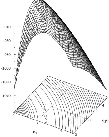
h=δt /100=0.0005 ky. Figure 5 displays the log-likelihood as a function of the noise levelsσ1andσ2calculated from the last sweep through the data. It turns out that approxi-mately models with the same valueτ2=σ₁2+σ₂2/γ2have the same likelihood; the likelihood contours in the(σ1, σ2/γ ) -plane are circles. The maximum of the likelihood is at a ra-dius of aboutτ =3.95. Moreover, models on the same like-lihood contour have the same scaled potentialV (z)/γ. From Eqs. (7) and (8), this is an indication that the system is in the limit of strong dissipation and models with the same effec-tive one-dimensional noise levelτ are equivalent. The exact value ofγ is ill-determined and depends on its initial esti-mate and uncertainty, but it is certainly very large (γ∼500– 1000).V (z)/γ andσ2/γare virtually independent of the pre-cise value ofγ. We can therefore fixγto an indicative value, sayγ=1000. Given that the partition of the noise amongσ1 andσ2does not matter here, we restrict our attention in the following to the caseσ1=0, that is, the classical Kramers problem.

For the ice-core data, the parametera1turns out to be ill-determined. This is probably a combined effect of the high noise level, the almost degenerate shape of the potential and

2

3

4 2

3 4 -1040

-1020 -1000 -980 -960 -940

σ₁

σ₂/γ

Fig. 5.Ice-core data: Log-likelihood as a function of the noise lev-elsσ1andσ2. Neighbouring contours differ by a factor of 100 in

likelihood.

-1050 -1000 -950

3 4 5

log-likelihood

σ2/γ, τ

Fig. 6. Ice-core data: Log-likelihood as a function of σ2/γ for

the oscillator model (solid) and as a function ofτ for the one-dimensional potential model (dashed).

the structural model error. The problem is removed by apply-ing the constraint that the mean state of the model matches the mean state of the data (cf. Kwasniok and Lohmann, 2009), that is,hzi =R∞

−∞zp(z)dz=0, leading to the

-0.4 -0.2 0 0.2 0.4

0 80 160 240 320 400

a4

/

γ

, a

3

/

γ

time [ky]

(a)

-2 -1 0 1 2

0 80 160 240 320 400

a2

/

γ

, a

1

/

γ

time [ky]

(b)

-4 -2 0 2 4 6

-4 -2 0 2 4

V(z)/

γ

, U(z), p(z)

z

(c)

Fig. 7. Ice-core data:(a)Estimates fora4/γ and a3/γ with

er-ror standard deviation. (b) Estimates for a2/γ with error

stan-dard deviation and estimates fora1/γ.(c)Scaled potentialV (z)/γ

for the oscillator model (thick solid) and potentialU (z) for the one-dimensional model (thick dotted). Probability densities of the ice-core data (solid), the oscillator model (dotted) and the one-dimensional model (dashed).

∞ Z

−∞

zexph−2γ V (z)/σ₂2idz=0. (25)

It is easily seen that, for fixed parametersa4,a3,a2,γ and noise levelσ2, the mean statehzi tends to +∞as a1 goes to−∞, tends to−∞as a1 goes to+∞, and has a mono-tonic dependence ona1in between. Thus Eq. (25) uniquely determinesa1for givena4,a3,a2,γ andσ2. The integral is evaluated numerically; the root is then found by running 15 iterations of the bisection algorithm starting with the interval

[−10,10]fora1/γ. The UKF is modified in that onlya4,a3 anda2are parameters to be estimated. We then haven=2,

-4 -2 0 2 4

20 30

40 50

60

δ

18

O anomaly [permille]

time [ky before present]

(a)

-4 -2 0 2 4

0 10 20 30 40

z

time [ky]

(b)

-4 -2 0 2 4

0 10 20 30 40

z

time [ky]

(c)

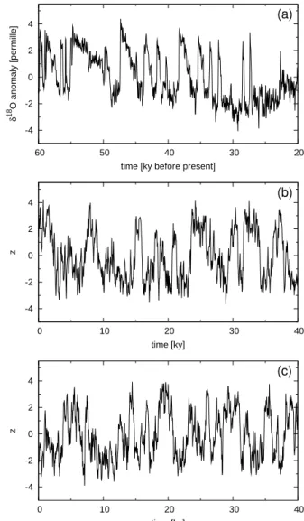
Fig. 8. (a)Record ofδ18O from the NGRIP ice core for the last glacial period with the mean value removed. (b) Sample trajec-tory of the oscillator model. (c) Sample trajectory of the one-dimensional potential model.

p=3 andna=5.a1is treated as a constant in the Kalman filter and updated according to Eq. (25) at each data point af-ter the Kalman update using the current estimates ofa4,a3 anda2.

Figure 6 shows the log-likelihood as a function ofσ2/γ. There is a maximum at σ2/γ=4 using a mesh of size 0.1. This is compared to directly fitting a one-dimensional Langevin model given by Eq. (1) with a potential U (z)=

P4

i=1aizi and a noise levelτ using the procedure of

slight overestimation ofσ2 in the simulated data. Figure 7 shows the parameter estimates and the derived potential. Averaging over the last sweep, the parameters area4/γ= 0.16±0.01,a3/γ= −0.22±0.02,a2/γ = −0.87±0.07 and

a1/γ=1.39. The potential is bistable and asymmetric; it has a deep well corresponding to the cold stadial state and a shal-low well corresponding to the warm interstadial state. The curvature of the potential givesγ /ω∗∼20≫1, confirming

that the system is clearly in the limit of strong dissipation. Also, when linearising the oscillator equation about the two equilibria of the potential, we get a damping ratio ofρ∼5 for the cold state andρ∼10 for the warm state, both far into the overdamped regime. The potential obtained by directly fitting a one-dimensional potential model is also given; it is virtually identical. The parameters then area4=0.17±0.01,

a3= −0.25±0.02,a2= −0.91±0.07 anda1=1.50. Fig-ure 7c also displays the stationary probability densities of the data and the two models; they are inflated by a factor of 25 to increase the readability of the plot. The probabil-ity densities were estimated using a Gaussian kernel estima-tor with the standard choice for the bandwidth (Silverman, 1986). Figure 8 gives sample trajectories of the oscillator model and the one-dimensional Langevin model contrasted with the anomaly ice-core record. As expected, the oscilla-tor model is statistically indistinguishable from the potential model.

6 Conclusions

We conclude that a Duffing-type oscillator model can be de-termined from the ice-core data, but it is in the regime of strong dissipation and can be very well approximated by a one-dimensional effective Langevin equation. The additional dynamics offered by Eqs. (3) and (4) over Eq. (1) is not actu-ally used by the system. The simpler one-dimensional model yields virtually the same likelihood as well as an equiva-lent potential and noise level. As already shown in Kwasniok and Lohmann (2009), such a model is able to capture some basic features of the ice-core record: the two modes of the probability density with approximately the correct popula-tion (Fig. 7c) as well as the amplitude and time scale of the switches between the stadial and interstadial state (Fig. 8). It cannot capture the pronounced temporal asymmetry of the DO events. A van der Pol-type relaxation oscillator might be more adequate here. But this is outside the scope of the present study and may be pursued elsewhere.

Edited by: R. Donner

Reviewed by: P. D. Ditlevsen and M. Crucifix

References

Alley, R. B., Anandakrishnan, S., and Jung, P.: Stochastic resonance in the North Atlantic, Paleoceanography, 16, 190–198, 2001. Alley, R. B., Marotzke, J., Nordhaus, W. D., Overpeck, J. T.,

Pe-teet, D. M., Pielke Jr., R. A., Pierrehumbert, R. T., Rhines, P. B., Stocker, T. F., Talley, L. D., and Wallace, J. M.: Abrupt climate change, Science, 299, 2005–2010, 2003.

North Greenland Ice Core Project members: High-resolution record of Northern Hemisphere climate extending into the last inter-glacial period, Nature, 431, 147–151, 2004.

Benzi, R., Parisi, G., Sutera, A., and Vulpiani, A.: Stochastic reso-nance in climatic change, Tellus, 34, 10–16, 1982.

Braun, H., Christl, M., Rahmstorf, S., Ganopolski, A., Mangini, A., Kubatzki, C., Roth, K., and Kromer, B.: Possible solar origin of the 1,470-year glacial climate cycle demonstrated in a coupled model, Nature, 438, 208–211, 2005.

Braun, H., Ditlevsen, P., and Kurths, J.: New measures of multi-modality for the detection of a ghost stochastic resonance, Chaos, 19, 043132, doi:10.1063/1.3274853, 2009.

Dansgaard, W., Johnsen, S. J., Clausen, H. B., Dahl-Jensen, D., Gundestrup, N. S., Hammer, C. U., Hvidberg, C. S., Steffensen, J. P., Sveinbj¨ornsdottir, A. E., Jouzel, J., and Bond, G.: Evidence for general instability of past climate from a 250-kyr ice-core record, Nature, 364, 218–220, 1993.

Dima, M. and Lohmann, G.: Conceptual model for millennial cli-mate variability: a possible combined solar-thermohaline circula-tion origin for the 1,500-year cycle, Clim. Dynam., 32, 301–311, 2009.

Ditlevsen, P. D.: Observation ofα-stable noise induced millennial climate changes from an ice-core record, Geophys. Res. Lett., 26, 1441–1444, 1999.

Ditlevsen, P. D., Kristensen, M. S., and Andersen, K. K.: The re-currence time of Dansgaard-Oeschger events and limits on the possible periodic component, J. Climate, 18, 2594-2603, 2005. Ganopolski, A. and Rahmstorf, S.: Rapid changes of glacial

cli-mate simulated in a coupled clicli-mate model, Nature, 409, 153– 158, 2001.

Ganopolski, A. and Rahmstorf, S.: Abrupt glacial climate changes due to stochastic resonance, Phys. Rev. Lett., 88, 038501, doi:10.1103/PhysRevLett.88.038501, 2002.

Gardiner, C.: Stochastic Methods, 4th Edn., Springer, 2010. Julier, S. J. and Uhlmann, J. K.: Unscented filtering and nonlinear

estimation, Proc. IEEE, 92, 401–422, 2004.

Julier, S. J., Uhlmann, J., and Durrant-Whyte, H. F.: A new method for the nonlinear transformation of means and covariances in fil-ters and estimators, IEEE Trans. Automatic Control, 45, 477– 482, 2000.

Kramers, H.: Brownian motion in a field of force and the diffusion model of chemical reactions, Physica, 7, 284–304, 1940. Kwasniok, F.: Estimation of noise parameters in dynamical

sys-tem identification with Kalman filters, Phys. Rev. E, 86, 036214, doi:10.1103/PhysRevE.86.036214, 2012.

Kwasniok, F. and Lohmann, G.: Deriving dynamical mod-els from paleoclimatic records: Application to glacial millennial-scale climate variability, Phys. Rev. E, 80, 066104, doi:10.1103/PhysRevE.80.066104, 2009.

Rial, J. A.: Abrupt climate change: chaos and order at orbital and millennial scales, Global Planet. Change, 41, 95–109, 2004. Sakai, K. and Peltier, W. R.: Dansgaard-Oeschger oscillations in a

coupled atmosphere-ocean climate model, J. Climate, 10, 949– 970, 1997.

Schulz, M., Paul, A., and Timmermann, A.: Relaxation oscilla-tors in concert: A framework for climate change at millennial timescales during the late Pleistocene, Geophys. Res. Lett., 29, 2193, doi:10.1029/2002GL016144, 2002.

Silverman, B. W.: Density estimation for statistics and data analysis, Chapman & Hall, 1986.

Sitz, A., Schwarz, U., Kurths, J., and Voss, H. U.: Estima-tion of parameters and unobserved components for nonlinear systems from noisy time series, Phys. Rev. E, 66, 016210, doi:10.1103/PhysRevE.66.016210, 2002.