i
EVALUATION OF SPATIAL INTERPOLATION TECHNIQUES
FOR MAPPING CLIMATE VARIABLES
WITH LOW SAMPLE DENSITY
A case study using a new gridded dataset of Bangladesh
ii
EVALUATION OF SPATIAL INTERPOLATION TECHNIQUES
FOR MAPPING CLIMATE VARIABLES WITH LOW SAMPLE
DENSITY
A case study using a new gridded dataset of Bangladesh
Dissertation supervised by
Professor Ana Cristina Costa, Ph.D
Coordinator of the Undergraduate Program in Information Management Instituto Superior de Estatística e Gestão de Informação
Universidade Nova de Lisboa, Portugal.
Professor Edzer Pebesma, Ph.D Professor and Director Institute for Geoinformatics University of Münster, Germany.
Professor Jorge Mateu, Ph.D Full Professor of Statistics Departamento de Matemáticas
Area de Estadística e Investigación Operativa Universitat Jaume I, Castellón, Spain
Professor Pedro Cabral, Ph.D
Assistant Professor and Program Leader of MSc in GIS & Sc Instituto Superior de Estatística e Gestão de Informação
Universidade Nova de Lisboa, Portugal.
iii
ACKNOWLEDGMENTS
“You don't write because you want to say something; you write because you've got something to say” - F. Scott Fitzgerald. I realize this one more time; when noteworthy contributions from a number of well-wishers craft me writing this dissertation acknowledgement.
The religious researchers always start with thanking god, I am an atheist; still I would like to start with thanking my god, my parents; to whom I am indebted from the day I was born, to nurture me up and to provide their every support in getting admitted to the Master of Science in Geospatial Technologies program and the successful completion of it with this thesis dissertation.
It is a pleasure to thank those who made this thesis possible, my supervisors – Professor Ana Cristina Costa, Ph.D; Professor Edzer Pebesma, Ph.D; Professor Jorge Mateu, Ph.D; and Professor Pedro Cabral, Ph.D; for their continuous support, idea-sharing, advice, guidelines, suggestions and comments to shape this thesis work from the beginning to the end. Their contributions not only helped me to carry out my research, but also to enlighten the tiny anthology of my wisdom.
Benedikt Gräler, he has made available his support in a number of ways to develop my thesis methodology; I would like to thank him for the support. My heartfelt thanks go to Professor Marco Painho, Ph.D; who helped me to structure my thesis work with his valuable comments during the seminar sessions.
I owe my deepest gratitude to Caroline Verena Wahle, who has started her contribution by providing me the means of survival during my stay in Germany for the second semester, and who finally turned into my beloved one. This thesis would not have been possible without her going through my draft manuscript for revision and correction by sacrificing time from her own job and thesis work.
iv
EVALUATION OF SPATIAL INTERPOLATION TECHNIQUES
FOR MAPPING CLIMATE VARIABLES WITH LOW SAMPLE
DENSITY
A case study using a new gridded dataset of Bangladesh
ABSTRACT
v
vi
KEYWORDS
Spatial Interpolation
Low Sample Density
Climate Change Index
vii
ACRONYMS
AR – Autoregressive
ARMA – Autoregressive Moving Average
BMD – Bangladesh Meteorological Department
CP –Confidence of Prediction
CV – Coefficient of Variation
IDW – Inverse Distance Weighting
IOC – Intergovernmental Oceanographic Commission
IPCC – Intergovernmental Panel on Climate Change
MA – Moving Average
MAE – Mean Absolute Error
MGC – Meteorological & Geo-Physical Centre
OK – Ordinary Kriging
PRISM – Partnership for Research Infrastructures in earth System Modelling
RADAR – Radio Detection and Ranging
RMSE – Root Mean Square Errors
RMSEs – Systematic Root Mean Square Errors
RMSEu – Unsystematic Root Mean Square Errors
SWC – Storm Warning Centre
TPS – Thin Plate Spline
UK – Universal Kriging
viii
INDEX OF THE TEXT
Page
ACKNOWLEDGMENTS ………. iii
ABSTRACT ………... iv
KEYWORDS ………. vi
ACRONYMS ………. vii
INDEX OF TABLES ………. xi
INDEX OF FIGURES ………... xii
1 INTRODUCTION ……….. 1
1.1 Background and rationale ……… 1
1.2 Research objectives ………. 2
1.3 Research scopes and propositions ………... 3
1.4 Structure of the manuscript ………. 4
1.5 Chapter conclusion ……….. 5
2 LITERATURE REVIEW ………... 6
2.1 Interpolating in space-time with climate variables ……….. 6
2.2 Sample density and estimation uncertainty ………. 7
2.3 Interpolation in space-time with low sample density ……….. 10
2.4 Chapter conclusion ……….. 14
3 STUDY AREA, DATASET AND CLIMATE CHANGE INDICES ……….. 15
3.1 Study area – Bangladesh ………. 15
3.2 Dataset and materials ………... 16
3.3 Climate change indices ……… 16
3.4 Low sample density problem to interpolate climate change indices ……... 20
3.5 Chapter conclusion ……….. 22
4 METHODOLOGY ………. 23
4.1 Spatial interpolation of climate change indices with low sample density ... 23
4.1.1 Deterministic spatial interpolation techniques ………... 24
4.1.1.1 Inverse Distance Weighting ……… 25
4.1.1.2 Thin Plate Spline ………. 26
4.1.2 Variography of climate change indices ……… 27
ix
4.1.3 Stochastic or geostatistical spatial interpolation ……….. 31
4.1.3.1 Ordinary Kriging ………. 32
4.1.3.2 Universal Kriging ………33
4.2 Evaluation of spatial interpolation techniques ……… 34
4.2.1 Willmott statistics ……… 35
4.2.2 Confidence of prediction ………. 36
4.3 Chapter conclusion ……….. 36
5 RESULTS AND DISCUSSION ……… 37
5.1 Search Neighborhood ……….. 37
5.2 Deterministic spatial interpolation results ………... 38
5.2.1 Thin plate spline surfaces ……….39
5.2.2 Inverse distance weighting surfaces ……….40
5.3 Stochastic spatial interpolation results ……… 40
5.3.1 Variography ………. 41
5.3.2 Ordinary kriging surfaces ……… 46
5.3.3 Universal kriging surfaces ………... 47
5.3.4 Differences among the surfaces created using different spatial interpolation techniques ………48
5.4 Performance evaluation of the spatial interpolation methods based on cross-validation ……… 49
5.5 Discussion of the results ……….. 53
5.6 Chapter conclusion ……….. 58
6 CONCLUSION AND FURTHER SCOPES ………. 59
6.1 Limitations and further scopes ……… 60
BIBLIOGRAPHIC REFERENCES ………. 61
ANNEXES ………. 71
A.1 TPS Surfaces of PRCPTOT ……… 71
A.2 IDW Surfaces of PRCPTOT ………... 77
A.3 OK Surfaces of PRCPTOT ……….. 82
A.4 UK Surfaces of PRCPTOT ……….. 87
A.5 Residual Plots of TPS Surfaces of PRCPTOT ……… 92
A.6 Residual Plots of IDW Surfaces of PRCPTOT ………... 96
A.7 Residual Plots of OK Surfaces of PRCPTOT ………. 100
A.8 Residual Plots of UK Surfaces of PRCPTOT ………. 104
A.9 TPS Surfaces of TXx ………... 108
A.10 IDW Surfaces of TXx ……….. 113
A.11 OK Surfaces of TXx ……… 118
A.12 UK Surfaces of TXx ……… 123
A.13 Residual Plots of TPS Surfaces of TXx ……….. 128
A.14 Residual Plots of IDW Surfaces of TXx ………. 132
A.15 Residual Plots of OK Surfaces of TXx ………... 136
x
A.18 Difference Surfaces between TPS and OK(TPS-OK) of PRCPTOT …….. 149 A.19 Difference Surfaces between TPS and UK (TPS-UK) of PRCPTOT ……. 154 A.20 Difference Surfaces between IDW and OK (IDW-OK) of PRCPTOT ….. 159 A.21 Difference Surfaces between IDW and UK (IDW-UK) of PRCPTOT ….. 164 A.22 Difference Surfaces between OK and UK (OK-UK) of PRCPTOT ……... 169 A.23 Difference Surfaces between TPS and IDW (TPS-IDW) of TXx ………... 174 A.24 Difference Surfaces between TPS and OK (TPS-OK) of TXx …………... 179 A.25 Difference Surfaces between TPS and UK (TPS-UK) of TXx …………... 184 A.26 Difference Surfaces between IDW and OK (IDW-OK) of TXx …………. 189 A.27 Difference Surfaces between IDW and UK (IDW-UK) of TXx ………… 194 A.28 Difference Surfaces between OK and UK (OK-UK) of TXx ………. 199 A.29 Performance measurements of the four methods from
cross-validation for interpolating PRCPTOT ……….. 204 A.30 Performance measurements of the four methods from
xi
INDEX OF TABLES
Table 2.1: Sample sizes and margin at different coefficient of variation described by LYNCH, and KIM (2010); N = sample size, z= score of divergence of the experimental result and cv = coefficient
of variation ………... 9 Table 2.2: Necessary sample size for 95% confidence intervals for the
coefficient of variation in selected situations described by
KELLEY (2007), with desired degree of assurance of achieving
a confidence interval no wider than desired ……… 9
Table 5.1: Variogram parameters estimated from the spatially shifted temporal points set of the experimental variograms of
PRCPTOT and of TXx for three temporal periods for ordinary
kriging interpolation ……….43
Table 5.2: Variogram parameters estimated from the spatially shifted temporal points set of the experimental variograms of
PRCPTOT and of TXx for three temporal periods for universal
kriging interpolation ……….45
Table 5.3: Correlation coefficient between different performance evaluation measures of the spatial interpolation techniques and coefficient of variation of samples for interpolating PRCPTOT and TXx ………… 54
Table 5.4: Comparison of the performance evaluation measurements between the ordinary kriging methods applied to create PRCPTOT surface of 2007 applying the individual variogram designed by available 32 spatial points and mean variogram designed by shifted 475 spatial points of the temporal period of 1993-2007 ……… 57
xii
INDEX OF FIGURES
Figure 1.1: Structure of the manuscript ………... 4
Figure 2.1: (a) Distribution of the samples and (b) clustering of the study area according to homogeneity of sample density in
DUMOLARD (2007). The hierarchical legend means the sub-regions 1-with a low density of points and a concentrated pattern 2-with a low density of points 3-with a concentrated pattern 4-with correct density and pattern of points and 5-with a good sample
(density + pattern) ………. 12
Figure 2.2: (a) Distance-correlation plot and (b) correlation functions of the velocity measurements for the first six stations in HASLETT, and RAFTERY (1989). Each cross at (a) corresponds to a pair of synoptic stations and the dots correspond to pairs which include Rosslare and show lower correlation than others. Rosslare also shows identical pattern in terms of autocorrelation at different
time lags at (b) ……… 13
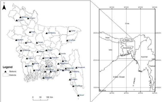
Figure 3.1: Study area – Bangladesh with world location and 34 meteorological stations to measure daily precipitation
and temperature (BHOWMIK and CABRAL, 2011).………... 15
Figure 3.2: Spatial trend PRCPTOT to southeast direction for all years, (a) decreasing trend with increasing latitude and
(b) increasing trend with increasing longitude ………..18
Figure 3.3: Spatial trend TXx to northwest direction - (a) increasing trend with increasing latitude and (b) decreasing trend
with increasing longitude ……….. 18
Figure 3.4: Temporal trend of (a) PRCPTOT and (b) TXx in every station
location ……….. 19
Figure 3.5: Temporal variability of PRCPTOT in every station location ………19
Figure 3.6: Temporal variability of TXx in every station location ………. 20
Figure 3.7: Vornoi polygons for prediction of continuous surface of TXx
by each meteorological station ………..21
Figure 4.1: Components of a typical variogram (KELKAR and PEREZ, 2002) ……. 28
xiii
Figure 4.3: Fitted variogram of the index PRCPTOT with (a) single temporal measurement at spatial points in 1956; and
(b) spatially shifted temporal measurements (1956-1980) …………31
Figure 5.1: Search Neighborhood for PRCPTOT estimation (nMax=32, nMin= 32) and for TXx estimation
(nMax=34, nMin=34) ………... 38
Figure 5.2: Inherent interpolation model by (a) thin plate spline method
(b) inverse distance weighting method ……….… 38
Figure 5.3: Increasing trend of number of stations available for
interpolating (a) PRCPTOT and (b) TXx ………. 41
Figure 5.4: Number of accumulated spatial points from spatially shifted
years to design variography for (a) PRCPTOT and (b) TXx ………41
Figure 5.5: Spatially shifted temporal points set of PRCPTOT for the temporal periods of (a) 1948-1975 (b) 1976-1992 and (c) 1992-2007 and of TXx for the temporal periods of
(d) 1948-1975 (e) 1976-1992 and (f) 1992-2007 ……….. 42
Figure 5.6: Mean variograms based on the parameters described in Table 5.1 using spatially shifted temporal points set of PRCPTOT for the temporal periods of (a) 1948-1975 (b) 1976-1992 and (c) 1992-2007 and of TXx for the temporal periods of (d) 1948-1975 (e) 1976-1992 and
(f) 1992-2007 for ordinary kriging interpolation ……….. 44
Figure 5.7: Mean variograms based on the parameters described in Table 5.2 using spatially shifted temporal points set of PRCPTOT for the temporal periods of (a) 1948-1975 (b) 1976-1992 and (c) 1993-2007 and of TXx for the temporal periods of (d) 1948-1975 (e) 1976-1992 and
(f) 1993-2007 for universal kriging interpolation ………. 46 Figure 5.8: Linear trends of the performance evaluation measurements
of the spatial interpolation methods: (a) (b)
(c) (d) (g) of the PRCPTOT
index; and (h) (i) (j)
(k) (n) of the TXx index
from 1948-2007 ……… 52
Figure 5.9: Linear trend of number of spatial points (n) and coefficient of variation (CV) of the sampled indices for (a) PRCPTOT and (b) TXx over years. CV has been rescaled to maintain
conformity with the number of spatial points to compare ………… 53
xiv
too big, different possible variograms (red, green, blue and yellow curves) are available for same
experimental variogram ……… 55
Figure 5.11: Variography designed with 32 available spatial points in 2007 to interpolate PRCPTOT using ordinary kriging
1
1. INTRODUCTION
“The choice of the appropriate methodology of interpolation of climatic data is crucial in order to obtain a correct representation of climatic fields”
- CRISCI, et al. 2006
The choice of appropriate spatial interpolation technique is a crucial research question
since there is no single preferred technique; rather the choice depends on the interpolation
performance in regards to the characteristics of the study area and data set. The question
becomes more critical since sample density of the irregularly distributed space-time
climate data has a significant effect on the spatial interpolation techniques in their
performance. The chapter outlines the rationale of the sample density impact research in
spatial interpolation performance analysis for the irregularly distributed space-time data
in light of existing researches. It describes and sorts out the research objectives and
propositions to carry out the entire research. It also structures the research manuscript
from this starting chapter to the concluding chapter.
1.1 Background and rationale
Spatial interpolation techniques have been used for mapping the spatial patterns of
climatic fields in several regions of the world, such as France (WEISSE, and BOIS, 2001), Germany (HABERLANDT, 2007), Great Britain (LLOYD, 2005), Italy (DIODATO, 2005), Mexico (BOER, et al., 2001; CARRERA-HERNÁNDEZ, and GASKIN, 2007), Portugal (DURÃO, et al., 2009; and
GOOVAERTS, 2000), and the United States of America (KYRIAKIDIS et al., 2001). There have
been a few studies conducted on the Bangladesh climate, based on the data from
meteorological stations; but so far no study has been conducted in Bangladesh to analyze
the spatial patterns of climate indices. This kind of study is very important since many
climate indices representing a wide variety of Asian climate aspects are already in the
phase of implementation. For example, SUHAILA and JEMAIN (2011) analyzed the spatial patterns of rainfall intensity and concentration indices over the Peninsular Malaysia.
Moreover, global continuous surface models of climate response are no longer useful for
practical reasons; international agencies, especially funding agencies are nowadays
asking for regional datasets of climate change from the developing countries for the
2
Spatial interpolation techniques have been profoundly used to quantify region-specific
climate change based on historical data (DIRKS et al. 1998). But since there is no single preferred technique for spatial interpolation, there is no local accurate interpolated surface
for mapping climate indices. Additionally, data unavailability and low sample density for
spatial interpolation have made the problem more complicated for the developing
countries. Recently it has been explored that for low-density datasets, complicated spatial
interpolation techniques do not show a significantly greater predictive skill than simpler
techniques (FRICH, et al., 2002; GOOVAERTS, 1998; and ISAAKS, and SRIVASTAVA, 1988). On the other hand, a high density climate dataset is not attainable for developing countries due to
techno-economic reasons.
Therefore, selecting the locally appropriate interpolation technique is very important for
mapping climate indices of Bangladesh in respect to very low density of sample. Yet the
problem of low sample density has not been properly addressed by the scientific
community. Though some of the authors have addressed the problem, the contribution is
insignificant (ANDERSON, 1987; and CHOWDHURY, and DEBSHARMA, 1992). Consequently, these issues motivated the research on an evaluation of the available interpolation techniques
based on the spatio-temporal characteristics of a climate dataset to analyze the climate
variability phenomenon for a low sample density region - Bangladesh. Two climate
indices have been selected, which are recommended by the Joint Project Commission for
Climatology/Climate Variability and Predictability (CLIVAR) and Joint WMO/IOC
Technical Commission for Oceanography and Marine Meteorology Expert Team on
Climate Change Detection and Indices (PETERSON et al. 2001; ZHANG, 2009), namely PRCPTOT and TXx. The PRCPTOT characterizes the annual total precipitation in wet
days, and the TXx corresponds to the yearly maximum value of the daily maximum
temperature.
1.2 Research objectives
The following research objectives have been established:
Exploration and Indices’ Pattern Analysis:
• To compile a rainfall and temperature dataset for Bangladesh.
3
• Investigate the spatial and temporal variability of the climate indices.
Uncertainty reduction in modelling and Interpolation:
• Prepare continuous surfaces with two alternative deterministic spatial interpolation techniques - Thin Plate Spline & Inverse Distance Weighting.
• Improve and model the experimental variograms for stochastic interpolation by providing them with enough pairs of points to model the spatial dependence in
response to low sample density.
• Prepare continuous surfaces with two alternative stochastic methods - Ordinary Kriging & Universal Kriging applying improved variograms.
Performance Evaluation and Sample-density Impact Analysis:
• Evaluate the interpolation cross-validation results by using suitable statistical performance measurements.
• Analyse the impact of low sample density on the performance measurements over time.
1.3 Research scopes and propositions
This research is aimed to evaluate the performance of spatial interpolation techniques
applied two most suitable and applicable indices that describe climate variability in
Bangladesh. The indices are calculated for each of the available years in dataset and
interpolated surfaces are then created. Additionally, the research is aspired to improve the
performance quality of the stochastic interpolation techniques. Most importantly, the
research is aimed to analyze changes in the performance of spatial interpolation
techniques with changing sample or spatial point density.
The following propositions are considered in the light of the described research scopes.
1. Sample or spatial point density does have a significant effect on the performance of spatial interpolation methods; the performance improves with the increase in
4
2. As a consequence of the dissimilar inherent methodology, different spatial interpolation techniques result in significantly different climate surfaces even
though they utilize the same climate dataset; but the difference decreases with the
increase in sample density.
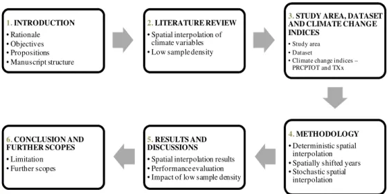
1.4 Structure of the manuscript
The manuscript consists of six chapters – Introduction, Literature Review, Study Area,
Dataset and Climate Change Indices, Methodology, Results and Discussion and
Conclusion and Further Scopes (Figure 1.1). The first chapter, introduction, outlines and
describes the research background, rationale, objectives and propositions. The second
chapter summarizes the literature that has been studied and describes them in the light of
spatial interpolation of climate variables and low sample density. The third chapter
introduces the study area and describes its important features. Furthermore, it describes
the dataset and climate change indices. It also illustrates the spatial and temporal trend of
the calculated climate change indices over the study area and study period. The fourth
chapter, methodology, explain see above the used methods for spatial interpolation
techniques and their performance evaluation. The fifth chapter describes the results that
have been obtained from the analysis implying the methodology, and shows the created
interpolated surfaces, their differences and estimation ability. It also explains the trend of
performance measurements over time with the increasing sample density. The final
chapter summarizes the findings from the study and outlines the limitations and further
scopes of the study.
1. INTRODUCTION
• Rationale • Objectives • Propositions • Manuscript structure
2. LITERATURE REVIEW
• Spatial interpolation of climate variables • Low sample density
3. STUDY AREA, DATASET AND CLIMATE CHANGE INDICES
• Study area • Dataset
• Climate change indices – PRCPTOT and TXx
4. METHODOLOGY
• Deterministic spatial interpolation • Spatially shifted years • Stochastic spatial
interpolation
5. RESULTS AND DISCUSSIONS
• Spatial interpolation results • Performance evaluation • Impact of low sample density
6. CONCLUSION AND FURTHER SCOPES
• Limitation • Further scopes
5
The manuscript also contains the bibliographic reference and thirty annexes at the end.
The bibliographic references list the literature that has been studied for the study and
which the information has been extracted from. The annexes contain created interpolated
surfaces by the four methods for the two climate change indices, their difference surfaces,
the residual plots and the performance measurement tables.
1.5 Chapter conclusion
This chapter has discussed in detail the research background and rationale followed by
the objectives and propositions. In a nutshell, the study is going to explore and analyze
the impact of sample density on the performances of spatial interpolation techniques.
Additionally, it is going to evaluate the performances of the four mentioned spatial
interpolation techniques to interpolate the two climate change indices. The main goal of
this study is to prove the propositions. The following chapter, literature review, is going
describe the concepts of spatial interpolation of climate variables with low sample
density; which will elaborate the concepts that have been mentioned in the objectives and
6
2. LITERATURE REVIEW
The inherent responsibility of the professionals who deal with climate and climate change
is to provide insights regarding climate variables at any place at any time. The crucial part
of this responsibility is to predict those variables at those places and times where
observations of the climate elements do not exist (TVEITO, 2007). The problem has become even more critical when it was proved by the climatologists that the global metric is for
climate change is no longer useful because climate effects are felt locally and they are
region-specific (CHOWDHURY, and DEBSHARMA, 1992). From this point of view, special skills and knowledge are required to predict and result in the most reliable value for the desired
climate information. As TVEITO (2007) presents, “traditionally this is done by using observed values at neighboring stations which are then adjusted for representativity,
terrain and other effects affecting the local climatology. Such estimates have usually been
carried out as single point calculations, often including subjective considerations based on
local knowledge and experience. Most of these estimates will not be consistently derived
and they are thereby not reproducible and cannot be regarded as homogenous. They are
therefore of limited value, for example, for advanced climate analysis.”
This chapter conceptualizes the application of spatial interpolation techniques to estimate
the climate variables at not-sampled locations. It also describes what could be an ideal
sample size for these spatial interpolations and how existing research has dealt with small
sample size and low sample density in this respect.
2.1 Interpolating in space-time with climate variables
Spatial interpolation techniques, as geostatistical estimation techniques, with their
inherent properties and applications, have successfully been implemented to combine
different georeferenced climate variables and parameters in such a way that it is now
possible to give consistently derived estimates at any place at any time (CHOU, 1997;
GOOVAERTS, 1998; ISAAKS, and SRIVASTAVA, 1989; JOURNEL, and HUIJBREGTS, 1978; PHILLIPS, et al.,
1992; and TABIOS, and SALAS, 1985). This is also because of the fact the interpolations
techniques deal with the most important property of climate variables – they have a
temporal extent along with a spatial extent (HUTCHINSON, 1995). CARUSO, and QUARTA (1998) have classified the techniques according to their fundamental hypotheses and
mathematical properties, which are entitled as “deterministic method, statistical method,
7
and combined method”. The application and performance of the classified techniques are
solely dependent on their research areas and algorithms and parameters used. Thus,
obtaining a universally appropriate spatial interpolation technique for a particular
application is impossible; rather locally an application oriented interpolation technique is
obtainable (XIN, et al., 2003). Additionally, this locally appropriate spatial interpolation technique selection is subject to the qualitative and quantitative analysis of the local
spatial data, their exploratory analysis and different stages of trial and errors with the
techniques which is commonly recognized as cross-validation. More precisely, the result
of the appropriate technique needs to be further examined for their accuracy (GOOVAERTS, 1997; andTVEITO, 2007).
Cressie (1991), Szentimrey (2002) and Szentimrey, et al. (2005) have suggested a range of
mathematical statistical and geostatistical (stochastic) models of spatial interpolation in
light of meteorological prediction. Among them, deterministic and stochastic methods
have turned out to be the most simplistic and reliable methods for climate variability
analysis. Recently it has been explored that for small sampled datasets, complicated
kriging methods (stochastic) do not show significantly greater predictive skill than
simpler techniques, such as the inverse square distance method (deterministic) (BHOWMIK, and CABRAL, 2011; and ISLAM, 2006).
2.2 Sample density and estimation uncertainty
Statisticians have been utilizing the concept of ‘Coefficient of Variation ( )’ as a
determinant of the sample size for statistical estimation with respect to the expected
confidence level (BELLE, 2008) for a long time. As BELLE (2008) indicated, the coefficient of
variation ( ) is a dimensionless number that quantifies the degree of variability in respect
to the mean. The sample coefficient of variation is calculated using the following
formula:
………...…….(4.i)
Where, is the sample standard deviation, which is the calculated square root of the
unbiased estimate of the variance, and is the sample mean. The value is sometimes
multiplied by 100 so that the ratio of the standard deviation to the mean is expressed in
terms of a percentage. Therefore, it is commonly accepted, if the coefficient of variation
8
been set as 50% (AFONSO, and NUNES, 2011) which means if the coefficient of variation of a sample set is more than 50% then the statistical estimation using these samples will end
up with high uncertainty in general which means the estimation is less accurate.
LYNCH, and KIM (2010) explain a way to prevent the curse of uncertainty due to the high
coefficient of variation, which is to adjust the sample size. They describe the relationship
among coefficient of variation, sample size and uncertainty with a mathematical function
which illustrates that when the coefficient of variation is higher, the sample size should
be high enough as well to reduce the uncertainly and obtain the accepted level of
confidence. They, in conclusion, have provided a table (Table 2.1) showing the required
number of samples for a certain level of coefficient of variation with corresponding
expected uncertainty. The table clearly shows that if it is objected to estimate with 95% of
confidence (which denotes that mean error of estimation should not be more than 5% of
sample mean), for a coefficient of variation of 20%, 43 samples are required but on the
other hand if the coefficient of variation is 80%, 693 samples are required for estimation.
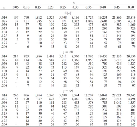
KELLEY (2007)describes asimilar concept like LYNCH, and KIM (2010), but in an elaborated
and functional way. He introduces some important parameters – expected confidence
interval width (E[w]), desired full confidence interval width (ω) and desired degree of
assurance (γ), to identify the level of confidence more precisely and then figures out the
required number of samples for estimation with expected uncertainty through a
mathematical function. As Table 2.2 illustrates, to estimate with 95% confidence where
the desired full confidence interval width is 10% (ω=0.10) and desired degree of
assurance is 99% (γ=0.99); if the coefficient of variation is 20%, 62 is the required
sample size and if the coefficient of variation is 50% then 401 samples are required to
estimate with expected confidence level.
Thus the sample size plays a significant role in statistics and so in geostatistics, since
estimating with reduced uncertainty is the explicit aim of any geostatistical analysis
(ISAAKS, and SRIVASTAVA, 1989). This is even more critical in interpolation since it’s required
to take into account the relative distances of the samples along with their values; for there
is a serious consequence of the property – “the global information carried by the
stationary mean becomes preponderant in prediction as remote neighboring data bring
less information about the unknown value at a distant location” (GOOVAERTS, 1997). This property along with the properties from LYNCH, and KIM (2010) and KELLEY (2007) clearly indicates the concept and problem of low sample density in spatial interpolation. Thus, if
the sample size is smaller than the minimum requirement for a desired confidence with an
9
inadequate samples, the interpolation results end up with a huge amount of unexpected
uncertainty and thus hamper the interpolation quality.
Even without coefficient of variation, sample size always determines the risk of
prediction (α value) for a constant variation in the samples, which is stated by
Chebyshev's Rule (OSTLE, and MALONE, 1990). Sample size and α value are always inversely proportional, so a decrease in the sample size always increases the risk of prediction. And
whenever the area of prediction increases the risk increases proportionally.
Table 2.1: Sample sizes and margin at different coefficient of variation described by LYNCH, and KIM
(2010); N = sample size, z= score of divergence of the experimental result and cv = coefficient of variation.
Table 2.2: Necessary sample size for 95% confidence intervals for the coefficient of variation in selected situations described by KELLEY (2007), with desired degree of assurance of achieving a
confidence interval no wider than desired.
GOULARD, and VOLTZ (1993) applied geostatistical interpolation methods to predict functions
at non-sample sites assuming that the functions were only known at a small set of points.
10
for penetration resistance of the soil. They applied a non-parametric fitting pre-process to
the observed functions where the smoothing parameter is chosen by functional
cross-validation. As such, smoothness improvement is a concern due to the existence of the low
sample density problem and in the case where the density of samples is significantly low
(even half or one third than the required sample size for expected confidence) the
interpolation and smoothness improvement need careful analysis and determination of the
variability function. The problem becomes even more critical when there is no possibility
to get enough points or a superimposing layer of high resolution remotely sensed dataset,
or other secondary data spatially correlated with the variable of interest which would
allow using an alternative multivariate technique for estimation and smoothness
improvement.
2.3 Interpolation in space-time with low sample density
In case of low sample density, spatial interpolations highly smooth the predictions, which
is especially undesirable for climate variables since climate variability is not smooth
neither perpetual. The smoothing basically depends on the local sample configuration, it
is minimal close to the sample locations and increases as the location of estimation gets
further away from the sample locations. Extensive smoothness of the interpolated surface
justifies the problem of low sample density.
The problem of interpolation with low sample density has been realized by the
geostatisticians in many cases (DIRKS, et al., 1998;HABERLANDT, 2007; PHILLIPS, et al., 1992; and
TABIOS, and SALAS, 1985), but no one has actually dealt with it. All of them have adopted the
classical approach of using auxiliary information in estimation, such as high resolution
datasets. HABERLANDT (2007) superimposed 21 measurements stations for extreme precipitation with a high resolution RADAR dataset and overcame the problem of
interpolation with small sample size.
The problem was actually addressed for the first time by DUMOLARD (2007) and TVEITO
(2007), though their focus was basically on the irregular distribution of the samples that
resulted in low sample density in some parts of their study areas. TVEITO (2007) eventually figured out that uncertainty of interpolation is a function of sample density and
uncertainty increases with the decrease in sample density. In the spatial interpolation of
temperature data, this author used well known as ‘residual kriging’ (detrended kriging)
which consists of two components – a deterministic model and a stochastic residual
11
temperatures were interpolated with different deterministic models for every month or
season. Finally the deterministic model was regionalized by predicting the model
parameters within a moving window and the remaining residual field was interpolated by
applying stochastic kriging method. Interpolating precipitation was more complicated
than temperature “since precipitation is non-continuous in space and time” (TVEITO, 2007).
DALY, et al. (1994) proposed the Precipitation-elevation Regression on Independent Slopes
Model (PRISM), which is based on local climate-elevation regression functions.
Long-term mean precipitation has been interpolated based on the principles of the
PRISM-method which (SCHWARB, 2001) incorporates different terrain characteristics - slope, aspect, etc. with a linear regression approach enabling the use of topographic information at
several spatial scales (DALY, et al. 2002; and 2006). SCHWARB (2001) combined radar information and in-situ observations to carry out further analysis.
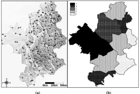
On the other hand, DUMOLARD (2007) dealt with a typical problem of sparsely distributed samples. He figured out that a simple linear regression between latitudes and longitudes
of the station locations for the 168 points gives a R² of 0.05 for an area of approximately
150,000 sq.km. And thus he found out that the probability α of a false rejection of
independence between X and Y is 0.044. What he worked out was giving a weak α = 0.01
risk, independence between latitude and longitude has been rejected but giving a larger
but reasonable α = 0.05 risk, it has been accepted. Finally, after introducing altitude and
creating the samples’ their ‘influence buffer’, he divided the entire study area into some
clusters with homogenous distribution of sample density and interpolated each cluster
separately and aggregating them to get the interpolation result of whole study area
(Figure 2.1). Thus he achieved a global improved accuracy by combining the uncertainty
of the local interpolation results since the cluster with higher sample density provided far
lower uncertainty than the low density clusters. The combined result also gave reduced
uncertainty than considering all samples of the study area as a whole.
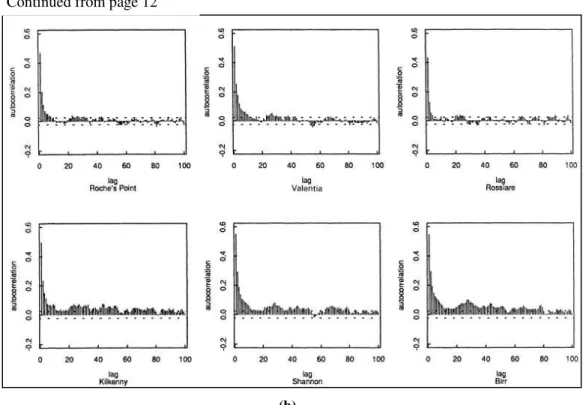
HASLETT, and RAFTERY (1989) compensated the fact of few spatial points in analysis with
high density of temporal points. They use long term hourly records of wind speeds at the
12 synoptic meteorological stations on a simple and parsimonious approximating model
which accounts for the main features of wind speeds in Ireland, namely seasonal effects,
spatial correlation, short-memory temporal autocorrelation and long-memory temporal
dependence. Based on the temporal autocorrelations of the station wind speed values and
distance correlation analysis of the seasonal effect analysis, they decided to take one
station (Rosslare) out of the variogram analysis since this station was acting as outlier
12
synthesizing deseasonalization, kriging, ARMA modelling and fractional differencing in
a natural way.
(a) (b)
Figure 2.1: (a) Distribution of the samples and (b) clustering of the study area according to homogeneity of sample density in DUMOLARD (2007). The hierarchical legend means the sub-regions
1-with a low density of points and a concentrated pattern 2-with a low density of points 3-with a concentrated pattern 4-with correct density and pattern of points and 5-with a good sample
(density + pattern).
For their case, simple kriging estimator performs well as a point estimator and ARMA
modeling as good interval estimator after fitting both estimators in space and time. The
cross-validation with the fitted models also resulted in significantly reduced errors which
encouraged considering temporal variability and dependence in interpolating with low
spatial density of samples. This means the low density in the spatial extent of the data and
resulted uncertainty due to that can be minimized by using the high density in the
temporal extent in creative ways.
(a)
13
(b)
Figure 2.2: (a) Distance-correlation plot and (b) correlation functions of the velocity measurements for the first six stations in HASLETT, and RAFTERY (1989). Each cross at (a) corresponds
to a pair of synoptic stations and the dots correspond to pairs which include Rosslare and show lower correlation than others. Rosslare also shows identical pattern in terms of autocorrelation at
different time lags at (b).
RAUDYS, et. al (1991) analyzed typically the influence of both training and testing sample size on the design and performance of pattern recognition system. They clearly proved
the existence of “curse of dimensionality” which implies that the classification accuracy
obviously increases with the increase in the number of sample; thus a large training
sample size is required for applications with large number of features and a complex
classification rule, and a large test sample size is required to accurately evaluate a
classifier with a lower error rate in cross-validation. It is true that classification and
interpolation are two different concepts apart from the fact that they both need to train
samples and evaluate their performance through cross validation. In interpolating
continuous variables, leave-one-out cross validation is typically used.
But still the following approaches they suggested to increase the classification accuracy
and to minimize estimation error from cross-validation seem even very useful for
interpolation.
1. Increasing the features and thus artificially preparing a sample size sufficient to
14
2. From the finite number of training samples carefully choosing those samples
which support to improve the design of spatio-temporal variability and discard
outliers.
The second approach implies to take out samples acting as outliers during model
preparation. In case of interpolating in space-time, more care is needed in this regard
since full stations along with their complete time series might be needed to be taken out.
Finally, DOBESCH, et al. (2001) indicated some important properties of interpolation results using the sparsely distributed and low density samples. They claim that the map of local
interpolated values of the variable will be smoothed if the variable is spatially continuous;
but the representativeness of the sample locally can be smoothed and mapped if
superimposed to the interpolated values and the global quality of the interpolation can be
assessed through an analysis of variance. The authors suggested “test several methods,
choose the right method, and correct use of the method and validation” as the sequence of
approaches to carry out the interpolation in space-time with low sample density and
reduced uncertainty.
2.4 Chapter conclusion
This chapter has presented a detailed overview of the preferred spatial interpolation
techniques by the scientific community for mapping climate variables. It has also
discussed the ideal size of sample for statistical estimation with acceptable accuracy.
Furthermore, various approaches by the geostatisticians to deal with the sample density
problem have been outlined. The next chapter, study area, dataset and climate change
indices, will describe the study area and dataset; calculate the two climate change indices
and analyse their behavior over space and time. The indices will be used as input of
15
3. STUDY AREA, DATASET AND CLIMATE CHANGE
INDICES
The characteristics and important features of the study area and dataset are key issues to
be considered in the choice of spatial interpolation techniques. There are specific spatial
interpolation techniques, which are developed to specifically apply in case of certain
features of the study area and dataset. This chapter outlines the important decision
making features to choose appropriate spatial interpolation techniques to evaluate. In
addition, it calculates and characterizes the two climate change indices that are used as
input for the spatial interpolation of the climate phenomenon.
3.1 Study area - Bangladesh
Bangladesh, situated in south-east Asia, is one of the most vulnerable countries of the
world regarding the adverse impacts of anthropogenic climate change (BRAUN, 2010; CAI, et
al., 2010; CHOWDHURY, and DEBSHARMA, 1992; KLEIN, et al., 2006; and SHAHID, 2009) (Figure 3.1).
The total area of the country is 147,570 square kilometer (BBS, 2009), approximately one fifth of which consists of low-lying coastal zones within one meter of the high water
mark (IPCC, 2007).
16
Threats of sea level rise, droughts, floods, and seasonal shifts due to global warming have
been presented in many recent studies on the country. The rainfall regime of the country
is highly variable in both time and space. The annual mean rainfall varies from 1400 mm
in the west to more than 4300 mm in the east of the country (SHAHID, 2010). The mean annual temperature has increased during the period of 1895-1980 by 0.310C
(PARTHASARATHY, et al., 1987) and the annual maximum temperature is predicted to increase by 0.40C and 0.730C by the year of 2050 and 2100 respectively (KARMAKAR, and SHRESTHA,
2000; and MIA, 2003). The Bangladesh Meteorological Department (BMD) is the
authorized government organization for all meteorological activities in the country. It
maintains a network of surface and upper air observatories, radar and satellite stations,
agro-meteorological observatories, geomagnetic and seismological observatories and
meteorological telecommunication systems. The department has its headquarter in the
capital Dhaka, with two regional centers – the Storm Warning Centre (SWC) in Dhaka
and Meteorological & Geo-Physical Centre (M & GC) in Chittagong. It measures the
daily precipitation and daily temperature with thirty-four meteorological stations situated
in different locations all over the country (DMICCDMP, 2012) (Figure 3.1).
3.2 Dataset and materials
The dataset used in this study includes daily precipitation and temperature measurements
from the meteorological stations of BMD for 60 years i.e. 1948-2007. The dataset is not
available from the beginning of the study period for all stations; precipitation data from 8
stations and temperature data from 10 stations is available for 1948 and there is a gradual
increase of precipitation data from 32 stations and temperature data from 34 stations by
2007 eventually. ‘Spacetime’, ‘intamap’, ‘fields’ and ‘gstat’ packages of the open source
statistical software ‘R’ (ISMWUWW), 2012) and ArcGIS version 10.0 (Esri, 2012) by Esri are utilized in order to analyze and compute the data.
3.3 Climate change indices
Two climate change indices – PRCPTOT and TXx (PETERSON et al. 2001; PLUMMER, et al.,
1999; Santos et al., 2011 and You et al. 2011) have been calculated from the available precipitation and temperature data for each year of 1948-2007 and for each station. These
climate change indices are internationally recognized and have been used in different
17
PRCPTOT refers to the annual total precipitation in wet days (PETERSON et al. 2001; and You et al. 2011). Since Bangladesh has clearly defined wet days in the year, the weather
phenomenon is known as ‘Monsoon’ and is present in June-September of every year
(ALEXANDER, 1999; BRAUN, 2010; MEF, 2008; IPCC, 2007; and WB, 2012), PRCPTOT is the most representative of change in precipitation. The formula for calculating PRCPTOT is:
if is the daily precipitation amount on day in period and if represents the
number of days in , then (PETERSON et al. 2001)
………….……..………(3.i)
TXx refers to the yearly maximum value of the daily maximum temperature (Peterson et al. 2001; and PLUMMER, et al., 1999). Previous studies have proven that the change in
temperature of Bangladesh due to climate change is more recognizable from the change
in maximum temperature (BRAUN, 2010; and CAI, et al., 2010). The formula for calculating
TXx is: if TXx is the daily maximum temperatures in period , then the maximum daily
maximum temperature each year is (PETERSON et al. 2001):
………(3.ii)
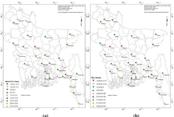
The calculated climate indices – PRCPTOT and TXx show spatial trends over the study
area (Figures 3.2 and 3.3). The PRCPTOT values increase with an increase in longitude
and decrease with an increase in latitude (Figure 3.2). This indicates that PRCPTOT
shows a spatial trend from the northwest to the southeast direction i.e. higher monsoon
precipitation is experienced in the southeast region of the country. The correlation of
PRCPTOT with longitude (0.55) is higher than the correlation of PRCPTOT with latitude
(-0.42), which indicates that the spatial trend is more dominant in west-east direction than
north-south direction. On the other hand, the TXx values increase with an increase in
latitude and decrease with an increase in longitude (Figure 3.3). This indicates that TXx
shows a spatial trend from the southeast to the northwest direction, i.e. a higher yearly
maximum of the daily maximum temperature is experienced in the northwest region of
the country. The correlation of TXx with longitude (-0.52) is again higher than the
correlation of TXx with latitude (0.34), which indicates that the spatial trend is more
dominant in the west-east direction than the north-south direction. It is important, since
Bangladesh is a flat country (KLEIN, et al., 2006), that the correlation of both PRCPTOT and TXx is insignificant with altitude and therefore height does not affect the spatial trend of
18
(a) (b)
Figure 3.2: Spatial trend PRCPTOT to southeast direction for all years, (a) decreasing trend with increasing latitude and (b) increasing trend with increasing longitude.
(a) (b)
Figure 3.3: Spatial trend TXx to northwest direction - (a) increasing trend with increasing latitude and (b) decreasing trend with increasing longitude.
The results of the analysis of the general temporal trend of the calculated climate change
indices are presented in Figure 3.4. For PRCPTOT, a range of -18 to 36 for the trend
value has been obtained. Most of the stations show an increasing trend of PRCPTOT over
time. Especially the stations in the southeast region of the country experience the highest
increasing trend, where the highest values of PRCPTOT are also experienced. On the
other hand, for TXx a range of -0.09 to 0.33 for the trend value has been obtained.
Though most of the stations show an increasing trend of TXx, almost all the stations in
the mid-region, including capital Dhaka, show a decreasing trend. The station at Rangpur
district, which represents the warmest region of the country (BBS, 2009), shows a decreasing trend of TXx. This fact indicates clearly that the climate is shifting, which will
19
(a) (b)
Figure 3.4: Temporal trend of (a) PRCPTOT and (b) TXx in every station location.
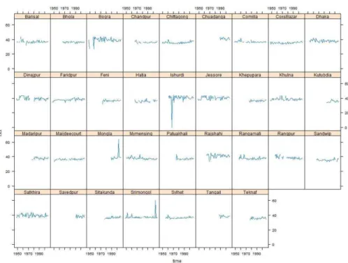
Detailed temporal variability of PRCPTOT and TXx in every station is presented in
Figures 3.5 and 3.6 respectively. It is difficult to predict any detailed temporal trend for
the indices, but the variability at some station locations show a trend in the index
behavior. It is obvious that the variability in the PRCPTOT index is more dominant than
in the TXx index.
Figure 3.5: Temporal variability of PRCPTOT in every station location.
P
R
C
P
T
O
20
Figure 3.6: Temporal variability of TXx in every station location.
The sudden increase and decrease in the variability are caused by the inconvenient data
quality, which could not be evaluated within this research scope. Figure 3.5 and 3.6 also
represent a lot of missing indices in the time series, which are occurred by the missing
data in the original dataset. The missing data has been considered as no data value in
calculation of the indices and thus the produced missing indices in the time series do not
take part in the spatial interpolation.
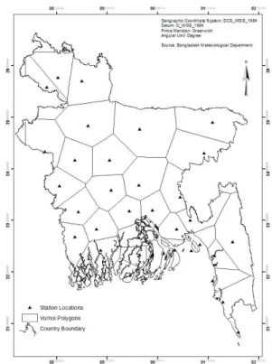
3.4 Low sample density problem to interpolate climate change indices
As described in chapter 2, like any statistical estimation, spatial interpolation requires a
sufficient number and density of samples to obtain acceptable accuracy. In light of this
discussion, interpolation of both PRCPTOT and TXx indices for Bangladesh experiences
the low sample density problem. Considering 34 meteorological stations which are
available in maximum in 2007 to interpolate TXx, each station is used to estimate the
continuous surface for 4340 square kilometer area, which is very big for a station to
estimate. Figure 3.7 represents the fact clearly; the size of the Voronoi polygons to
estimate is very big. The R2 value of simple linear regression between latitude and
longitude of the stations is 0.339 which is good from the perspective described in
21
But the risk of estimation α for TXx is 0.008 when the sample size is 34, but α decreases
to 0.000006 if the sample size is increased to 100, when other parameters remain constant
according to TVEITO (2007). This indicates that the number of stations is too little to interpolate with acceptable accuracy.
Figure 3.7: Vornoi polygons for prediction of continuous surface of TXx by each meteorological station.
Furthermore, interpolation methods will highly smooth the predictions in the presence of
low sample density, which is undesirable for climate data. The global information carried
by the stationary mean becomes preponderant in prediction as remote neighboring data
bring less information about the unknown value at a distant location (GOOVAERTS, 1997). Consequently, the smoothing effect is minimal close to the data locations and increases as
the location being estimated gets farther away from data locations. On the other hand,
according to AFONSO, and NUNES (2011), if the coefficient of variation is high, the mean will
not be representative of the attribute behavior. The coefficient of variation ( ) of samples
for PRCPTOT is 41% in average and ranges from 25% to 59%, while for TXx it is 6.2 %
and ranges from 3.2% to 24%. Therefore, the mean will not be representative of the
PRCPTOT behavior in many years; for TXx the attribute's variability is not so
pronounced, but it might have the same problem as PRCPTOT in a few years. Moreover,
according to these values, to interpolate and produce continuous surfaces with 95%
22
sample size for PRCPTOT is 173 on average which may vary from 43 to 390, and it is
equal to 4 on average for TXx which may vary between 1 to 43 as described in LYNCH, and
KIM (2010). As explained in KELLEY, (2007), to estimate with 95% confidence where the
desired full confidence interval width is 10% (ω=0.10) and desired degree of assurance is
99% (γ=0.99), the required sample size to interpolate PRCPTOT is 16,233 and to
interpolate TXx is 199. For both cases, the number of samples or spatial points is too low
to obtain acceptable accuracy.
3.5 Chapter conclusion
As presented in this chapter, the sample density of the study region is too low to provide
acceptable accuracy in the spatial interpolation results. The calculated indices behavior
over space and time and the features of the study area lead to the decision of evaluating
possible deterministic and stochastic spatial interpolation techniques. As ATKINSON, and
TATE, 2000; and ISAAKS, and SRIVASTAVA, 1988 discovered, that in case of uncertain
sample distribution and size, deterministic methods should be the preferable options for
spatial interpolation, two deterministic methods – Thin Plate Spline (TPS) and Inverse
Distance Weighting (IDW) can be applied for interpolation of the indices. The two
deterministic methods fit the interpolation models exactly through the measured points,
but TPS performs some degree of smoothing and IDW performs with no smoothing. On
the other hand, two stochastic methods can be applied after improving the variograms to
fit the models – Ordinary Kriging (OK) and Universal Kriging (UK). The OK model can
be applied taking the anisotropic behavior of the indices into account, while UK can be
applied by taking the spatial trend of the indices into account. The following chapter,
methodology, will describe the spatial interpolation models in detail, derived from the
literature review and fitting to the dataset. It will also outline the methods for the
23
4. METHODOLOGY
This chapter describes the detailed methodology of the four spatial interpolation
techniques and their rationale of application for the study area and dataset. It elaborates
the spatial interpolation models with mathematical equations fitting to the study area and
climate change indices. It also outlines seven different performance measurements to
evaluate the performances of these spatial interpolation techniques and their importance.
4.1 Spatial interpolation of climate change indices with low sample
density
Spatial interpolation of climate change indices needs special spatialization since the
indices contain both spatial and temporal information inherently (TVEITO, 2007). In practice, the spatial interpolation techniques that incorporate temporal information with
spatial information in the modeling function are most appropriate for interpolating
climate variables (HASLETT et al., 1989; and TRENBERTH et al., 2000). The structure of a basic spatial interpolation problem denotes that denotes that the dependent variable of interest
is predicted as an output of the mathematical function of known predictors
, where the location vectors are the elements of the given space
domain and is time. The vector form of the predictors is
(SZENTIMREY et. al., 2007). The probability distribution of the climate variables sets up the appropriate interpolation formulae, which
include some unknown interpolation parameters. These parameters can be obtained
through known functions of certain statistical parameters. Modeling of climate variables
with these statistical parameters assume that the expected values of the variables are
changing in space and in time in a similar way (CHRISTAKOS, 2001; TVEITO, 2007). The spatial change in the variables indicates that the climate is different in the regions
whereas temporal change is considered as the result of climate variability or of possible
global climate change (HIJMANS et. al, 2005). As a result, expected values of climate variables can be obtained by the following linear model (CHRISTENSEN, 1990; PAPRITZ and
STEIN, 1999):
24
Where, is the temporal trend or the climate change signal, is the spatial trend.
Typically, there is only a single realization in time for the modeling of the statistical
parameters in spatial interpolation. Therefore only the predictors
constitute the usable information or the sample for the modeling of variability over space
(SZENTIMREY et. al., 2007).
At the linear model (4.i), the basic statistical parameters can be allocated into two
categories - deterministic and stochastic parameters. Thus the spatial interpolation
techniques can be divided into two groups – deterministic and stochastic spatial
interpolation techniques (CHRISTAKOS, 2001; and SZENTIMREY et. al., 2007).
4.1.1 Deterministic spatial interpolation techniques
Deterministic interpolation techniques create surfaces from the predictors by a
mathematical function of the extent of similarity or the degree of smoothness (WEBSTER
and OLIVER, 2001; BHOWMIK and CABRAL, 2011). In linear equation (4.i), the deterministic or
local parameters are the expected values . If denotes the
vector of expected values of predictors, then the linear model for deterministic
interpolation will be (SZENTIMREY et. al., 2007):
………(4.ii)
The two climate change indices of the study can be modeled deterministically in the
manner adopted by HANCOCK and HUTCHINSON (2005). The indices are considered as data
observations measuring a dependent variable and predictor
variables which are included ina set of space domain . These climate
change indices are often well predicted using latitude, longitude and altitude. If has
both continuous long range variation as well as discontinuous and random short range
variation, then the data model can be expressed as:
………(4.iii)
Where, is the number of data observations, is a slowly varying continuous function
and is the realization of a random variable . The function represents the spatially
continuous long range variation in the process measured by . The errors of are
25
the measurement error and short range microscale variation that occurs over a range
smaller than the resolution of the data set. The microscale variation may be spatially
continuous, but the low spatial density of dataset (as discussed in literature review and
study area, dataset and climate change indices chapters) is unable to represent it. That is
why it is assumed as discontinuous noise of the data (TRENBERTH et al., 2000).
Therefore two deterministic approaches based on linear equation (4.ii) can be fitted to the
data model of (4.iii). The Inverse Distance Weighting (IDW) approach predicts the
dependent variable based on the extent of similarity, whereas the Thin Plate Spline (TPS)
approach predicts it based on the degree of smoothing (JOURNEL and HUIJBREGTS, 1978).
4.1.1.1 Inverse Distance Weighting
The inverse distance weighting method predicts the process in (4.iii) by giving more
weight to nearby measurements than to distant measurements. The analytical expression
of the surface can be expressed as (CARUSO and QUARTA, 1998):
……….………(4.iv)
where, is the number of measurements, is the measurement value, is the
Euclidean distance with point , and is the weighting function. The weighting
function can be adjusted by the following formula:
……….…(4.v)
Where is minimum distance, is the maximum distance from the location
being predicted. Index prevents infinite weight values for . If no point falls
into the circle of radius , average measurement value is taken (VICENTE-SERRANO et
al., 2003).
Taking (4.iv) and (4.v) into account, the linear model 4(ii) can be written as following
26
, ..(4.vi)
4.1.1.2 Thin Plate Spline
The thin plate spline (TPS) method predicts the process in 4(iii) by a suitably
continuous function that is able to separate the continuous signal from the
discontinuous noise (HANCOCK and HUTCHINSON, 2005). This function can be estimated by minimizing
…………...……….…(4.vii)
over functions , where is a space of functions whose partial derivatives of total
order are in (WAHBA, 1990; HANCOCK and HUTCHINSON, 2005). The are values
of the fitted function at the th measurement, is a fixed smoothing parameter, and
is a measure of the roughness of the function in terms of th order partial
derivatives. The form of depends on and the number of independent variables
. For the typical value , , then can be modeled as (CHRISTAKOS,
2001):
…………...…(4.viii)
Equation (4.viii) represents an exchange between fitting the data as closely as possible
whilst maintaining a degree of smoothness (HANCOCK and HUTCHINSON, 2005). The
smoothing parameter controls the separation of long range and short range variation. If
, the function accurately interpolates the data, implying zero noise and when
is very large, the function approaches a hyperplane. The corresponding to the spline
function that best represents the underlying process can be predicted by minimizing
the generalized cross validation (GCV) (CHRISTAKOS, 2001; and HANCOCK and HUTCHINSON,