SHORT-TERM VARIABILITY AND TRANSPORT OF NUTRIENTS AND
CHLOROPHYLL-A IN BERTIOGA CHANNEL, SÃO PAULO STATE, BRAZIL
Sônia Maria Flores Gianesella1, Flávia Marisa Prado Saldanha-Corrêa1, Luiz Bruner de Miranda1, Marco Antonio Corrêa2 & Gleyci Aparecida Oliveira Moser3
1
Instituto Oceanográfico da Universidade de São Paulo (Praça do Oceanográfico, 191 CEP 05508-120, São Paulo - SP, Brasil)
2
ASA-South America
(Rua Purpurina, 155 CEP 05435-030, São Paulo, SP, Brasil)
3
Centro Universitário Monte Serrat Faculdade de Ciências Ambientais- Oceanografia
(Av. Saldanha da Gama, 89, Santos, SP, Brasil) Corresponding author: soniag@io.usp.br
A
B S T R A C TShort-term variability of nutrients, chlorophyll-a (Chl-a) and seston (TSS) concentrations were followed up at a fixed station in the Bertioga Channel (BC), Southeastern Brazil, over two full tidal cycles of neap and spring tides, during the winter of 1991. Simultaneous data on hydrographic structure, tidal level and currents allowed the computation of the net transport of those properties. Tidal advection and freshwater flow were the main forcing agents on the water column structure, nutrient availability and Chl-a distribution. Dissolved inorganic nitrogen and phosphateaverage values were high (16.88 and 0.98 µM, respectively, at neap tide and 10.18 and 0.77µM at spring tide). Despite N and P availability, Chl-a average values were low: 1.13 in the neap and 3.11 mg m-3 in the spring tide, suggesting that the renovation rate of BC waters limits phytoplankton accumulation inside the estuary. The highest Chl-a was associated with the entrance of saltier waters, while the high nutrient concentrations were associated with brackish waters. Nutrients were exported on both tides, TSS and Chl-a were exported on the spring tide and Chl-a was imported on the neap tide. The study of the main transport components indicated that this system is susceptible to the occasional introduction of pollutants from the coastal area, thus presenting a facet of potential fragility.
R
E S U M OVariações de curta escala das concentrações de nutrientes, clorofila-a (Cl-a) e séston foram acompanhadas em uma estação fixa no canal de Bertioga (CB), sudeste do Brasil, em dois ciclos completos de maré de quadratura e sizígia, no inverno de 1991. Dados simultâneos da estrutura hidrográfica, marés e correntes permitiram calcular o transporte resultante daquelas propriedades. A advecção por maré e o fluxo de água doce foram as principais forçantes da estrutura hidrográfica e da distribuição de nutrientes e Cl-a. As concentrações médias de NID e fosfato foram altas (respectivamente: 16,88 e 0,98 µM na quadratura e 10,18 e 0,77 µM na sizígia). Apesar da disponibilidade de N e P, os valores médios de Cl-a foram baixos: 1,13 mg m-3 (na quadratura) e 3,11 mg m-3 (sizígia), sugerindo que a alta taxa de renovação das águas do CB limitam o acúmulo de fitoplâncton. Os maiores valores de Cl-a relacionaram-se à entrada de águas costeiras enquanto que as altas concentrações de nutrientes foram relacionadas às águas salobras. Os nutrientes dissolvidos foram exportados em ambas as marés, séston e Cl-a foram exportados na sizígia e, na quadratura, a Cl-a foi importada. O estudo dos principais componentes do transporte indicou uma susceptibilidade desse sistema à introdução de poluentes oriundos da área costeira, revelando uma potencial fragilidade ambiental.
Descriptors: Inorganic nutrients, Chlorophyll-a, Séston, Tidal cycle, Transport components, Outwelling, Bertioga Channel, Estuary.
Descritores:Nutrientes inorgânicos, Clorofila-a, Séston, Ciclo de maré, Componentes do transporte, Exportação, Canal de Bertioga, Estuário.
__________
I
NTRODUCTIONEstuaries are considered highly productive environments and are significant routes by which terrestrial materials enter the ocean. Tides are major agents of transport in most coastal environments. Efforts to understand and quantify the interactions across the land-ocean boundary have led to an increasing focus on the fluxes of active biogeochemical components through estuarine systems (Simpson et al., 2001). To understand estuarine hydrodynamics and transfer processes it is important to have some reasonable knowledge of the fraction of the total longitudinal flux related to non-advective tidal processes and that related to non-advective gravitational circulation processes (Officer & Kester, 1991). These factors are specially important when it one is dealing with studies of water quality, biogeochemical oxygen demand, pollutant dispersion and eutrophication, which depend on estuarine hydrodynamics. From a physical point of view the deposition of fluvial material in estuaries depends on the gravitational circulation pattern and on basin morphometry, but processes such as flocculation are also important (Schubel & Kennedy, 1984). Flushing time is a further important characteristic of estuaries as it greatly affects the speciation of various dissolved substances and ultimately determines the quantity of constituents that reach the sea (Wollast, 1983).
There are several studies on the fluxes of materials such as suspended solids, phytoplankton and nutrients in temperate and tropical estuaries. General conceptual models of land-sea interface processes have been developed on the basis of a large body of knowledge from the temperate northern hemisphere (Eyre, 1998). In Brazilian estuaries, apart from the LOICZ program data (http://data.ecology.su.se/MNODE/), there are few studies focusing on the transport of properties, but among them are the studies of salt transport (Miranda & Castro, 1996) and iron and silicate (Barrera-Alba et al., 2002) in the Cananéia estuary, salt (Miranda et al., 1998) in the Bertioga channel, salt, inorganic nutrients, seston and chlorophyll transport in the Camboriú River (Pereira Filho et al., 2001) and the Santos estuary (Moser et al., 2005). The studies of Miranda & Castro (1996) and Miranda et al. (1998) were the only ones to have evaluated the relevance of the main transport components. The present work aims to describe spring and neap tidal forcing on the variation in nutrients and phytoplankton and their net transport based on the temporal series (26h) obtained at a fixed station in the BC (Fig. 1) during the dry season. The study focuses on the contribution of each transport component to total nutrients, TSS and Chl-a transport, in the attempt to establish their relative ecological importance.
Study Area
The Bertioga Channel (BC) belongs to the Santos estuarine complex system (Fig. 1) located on the central coast of São Paulo State, southeastern Brazil. In spite of the dense urban and industrial occupation and the port activities in the neighboring Santos estuary, the banks of the Bertioga Channel are still dominated by mangrove forest. The waters of its northern portion present little influence of the polluted Santos estuary due to the hydrodynamic characteristics of the area: since the Largo do Candinho, the wide central portion, acts as a water divisor between the two inlets. The whole channel (Lat. 23°50´ to 23° 56´S - Long. 46°7.9´ to 46°19´W) is 25 Km long and 460 m wide on average (Harari & Camargo, 1997) andhas several freshwater tributaries, the most important being the Itapanhaú River, with a mean discharge of 10 m3s-1 (Miranda et al., 1998). The pluviometric cycle is characterized by high precipitation in summer and a lower one in winter, with the absence of any marked dry season (DAEE, 2005).
The hydrographic characteristics of the northern portion of the BC (from the Largo do Candinho downstream) were studied by Miranda et. al. (1998) who classified this portion of the channel as a microtidal and partially mixed estuary with semi-diurnal tides and a pronounced fortnightly neap to spring tidal modulation, alternating from highly stratified (type 2b, sensu Hansen & Rattray, 1966) at neap tides, to moderately stratified (type 2a) during spring tides. Freshwater discharge varies from 40 to 19 m3 s-1 as between neap and spring tides while the flushing times are 2.1 d (4.1in neap tidal cycles) and 4 d (7.7 in spring tidal cycles) respectively, resulting in a renovation rate of 24.6% and 12.9% of the total water volume according to the tidal cycle. Gianesella et al. (2000) have studied nutrient, Chl-a and phytoplankton distribution along the longitudinal axis from the Largo do Candinho up to the Barra de Icapara. They verified a high nutrient concentration (up to 25 µM of ammonium), low dissolved oxygen saturation (minimum 20%) and low phytoplankton biomass in the upper reaches (0.5 to 1.5 mg m-3). The highest Chl-a levels were associated with waters of coastal origin and flood periods (maximum 4.5 mg m-3).
M
ATERIAL ANDM
ETHODSthe austral winter of 1991. Hydrographic properties and current measurements were taken hourly at every one-meter depth along the water column (mean depth was around 5.5 m). Temperature was measured with a reversing thermometer and salinity was estimated using the conductivity ratio (in water samples collected in Nansen bottles) converted to salinity according to the UNESCO Practical Salinity Scale (1981). Nearly simultaneous current speed and direction were measured with a mini Sensor Data current meter (model SD-4), and decomposed into longitudinal and transverse velocity components. The tidal level was recorded with a float and stilling well tide gauge positioned near the site of the fixed station. This hydrographic data set was analyzed and the physical characterization and salt transport computations have been reported in Miranda et al. (1998).
Water samples for chemical and biological analyses were taken hourly at the surface and one meter above the bottom with Van Dorn bottles. Dissolved oxygen (DO) was analyzed by the Winkler method (Grasshoff et al., 1983) and the results were presented as dissolved oxygen saturation (DOS)
according to UNESCO (1973). Inorganic nutrients were analyzed according to the methods described in Aminot & Chaussepied (1983) for ammonium, nitrate and nitrite and in Grasshoff et al. (1983) for phosphate and silicate. Euphotic zone thickness Zeu was
estimated by means of Secchi disk readings (Poole & Atkins, 1929).
The chlorophyll-a concentration (Chl-a) in 90% acetone extracts was estimated with a Turner 111 fluorometer (Yentch & Menzel, 1963; Holm-Hansen et al., 1965) and the percentage of the active fraction related to total pigment (Chl-aact / Chl-aact + Phaeo)
was calculated. Seston (TSS) was analyzed by the gravimetric method (APHA, 1985), for the spring tide only.
Based on the assumption that the BC is laterally homogeneous, the time series of the longitudinal velocity component (u), nutrients, Chl-a, Chl-aact and TSS were used to estimate the transport of
these properties. Although nutrients and Chl-a are not conservative properties, their sources/sinks by chemical and biological processes have been neglected in the calculation, for two main reasons:
1. The ranges of variation observed both at neap and spring tides were large and clearly related to the water source, whether salt or brackish.
2. Possible changes in nutrient or Chl-a
concentrations due to sources/sinks tend to be small, considering the short time scale of the observation period (26 h).
The instantaneous advective mass transport of a property (TC (t)), through a unit width of a section normal to the longitudinal flow of the estuarine channel is equal to:
H
uC
dz
uC
t
T
HC
=
∫
ρ
=
ρ
0
)
(
)
(
, (1)where ρ is the density (which was considered constant and equal to 1,000 Kg m-3), u is the longitudinal velocity component (u>0 down estuary, in m s-1), C is the property concentration (in g Kg-1 or mg Kg-1) and H=H(t) the depth (in m). The bar denotes the variable mean over the total depth.
The mean resultant transport <TC>over one
or more complete tidal cycles (T) is given by:
H
uC
dt
t
T
T
T
TC
=
∫
=
ρ
0
C
(
)
1
, in units of g
m-1 s-1 (2)
The time-space average value for the u
component is given by
u
and may be theapproximate value of the velocity component generated by the freshwater flow
u
≅ Q/A, where Q and A are the freshwater discharge and the transverse section area, respectively.Following a similar procedure to that elaborated by Bowden (1963), Dyer (1974) and Hunkins (1981), among others, the velocity and salinity may be decomposed into terms which represent the physical processes responsible for the advective and dispersive mass transports. This is done by separating the tidal influence (barotropic and time dependent) from that associated with the gravitational circulation (baroclinic and steady).
For a laterally homogeneous channel this decomposition is given by:
)
,
(
u'
)
(
u
)
(
u
)
,
(
u
z
t
=
u
+
tt
+
zz
+
z
t
(3)Where:
u
= freshwater discharge;u
-u
u
t=
(barotropic);u
u
u
z=
−
(baroclinic);z t
z,t
)
u
u
u
u(
u'
=
−
−
−
(turbulent fluctuation).Equivalently for the concentration:
)
,
(
C'
)
(
C
)
(
C
)
,
(
C
z
t
=
C
+
tt
+
zz
+
z
t
(4)
The depth at the fixed station is given by H that may be decomposed into:
H(x, t)= H0 + ξt(x, t) (5)
where H0 is the time-averaged water depth and ξt(x, t)
is the tidal height.
Substituting equations 3, 4 and 5 in equation 2:
(
u u u')
(
C C C')
( )) ( 1 0 0 C t z t z t T C H C u H uC dt t T T T
ζ
ρ
ρ
+ + + + + + + = = =∫
(6) According to this procedure the advective property transport, under steady conditions, is decomposed in 32 terms. Many of these terms disappear or may be neglected upon forming averages over depth and time. Ignoring other terms, for which there is no physical reason to expect correlations between steady, tidal and deviation components, seven main terms remain to explain total property transport through a unit of cross-sectional width under nearly stationary conditions: + + ′ + + + + = t t z t z z t t t t C C u C u H C u H C u H C u C u C u Tξ
ξ
ξ
ρ
0 0 0 0 ´ H (7)R
ESULTSClimatic conditions during the sampling period for both tides were typical for winter with a monthly rainfall of 156.1 mm (DAEE, 2005).
The most evident characteristic in the vertical profiles of salinity and nutrient time series is the alternation of periods of high and low vertical stratification related to the tidal phase (ebb or flood respectively), both in the neap and spring tides. Vertical density stratification was primarily due to salinity gradients. Further, high nutrient concentrations were associated with brackish waters.
Neap Tide Series
Temperature variation was small (Table 1), following the same pattern displayed by the salinity: at high water, the 20° C isotherm and 32.0 isohaline reached 1 m depth, dipping at ebb phases (Figs. 2a, b, c). Haline stratification was marked, especially at the flood slack tides, as a consequence of the intense coastal water intrusion at intermediate depths, as indicated by current speed profiles (Figs. 2 b and c). According to Miranda et al. (1998) the strongest flood currents (up to -0.6 m s-1) appear as subsurface velocity cores, located at around 2.5 m depth, preceding high water by 2-3 h. During the ebb tide, the longitudinal velocity component reaches its greatest speed (0.6 to 0.9 m s-1) as surface cores 3-4 h ahead of
low water. The current reversal lags high and low water by 1-2 h, and the slack tide did not occur simultaneously throughout the water column.
The mean DOS value was 59.6%, indicating the overall oxygen-undersaturated state of the waters especially at flood slack tides (Table 1, Fig. 2d). The lack of photosynthesis, OD uptake by respiration
processes and also the lower current speeds caused the DOS decrease detected in the entire water column in the period between 13 and 18 h in the series (night period from 2 to 7 a.m.). Due to the evident non-conservative behavior of this variable even on short time scales, its transport has not been calculated in the present study.
Euphotic zone thickness (Zeu) ranged from
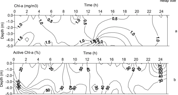
2.4 to 4.7m and occupied most of the water column, once the local mean depth was around 5.5 m (Fig. 2e). Minimum values were related to the action of higher current speeds in the bottom layers, which probably suspended sediments, thus enhancing water turbidity. Dissolved nutrient temporal variation was closely related to the tidal cycle. Surface brackish waters generally displayed higher nutrient concentrations than bottom waters, which were under the influence of the coastal water salt wedge (Figs 3a to 3f). The lower nutrient concentrations along the water column were recorded at high water. Nitrate and ammonium were the main nitrogen forms and displayed a wide range of variation (Table 1), related to water origin. The N:P ratio series indicated a phosphorous deficiency related to total DIN (NO3
-+NO2
-+NH4 +
) concentrations (ratios higher than 16:1) in inner channel waters, while the saltier waters displayed an excess of phosphate (Fig. 3f).
The phytoplankton biomass was low (Table 1), considering the high nutrient availability (Fig. 4a). Greater Chl-a concentrations occurred only in bottom waters during floods, or under salt-water influence. The proportion of Chl-aact was also higher in bottom
waters (Fig. 4b). The mean value computed for the entire period was 40% (Table 1), which is within the normal range for coastal regions.
Table 1- Mean values, standard deviation and range of variation of the physical, chemical and biological variables monitored along two tidal cycles in a neap and a spring tide at a fixed station in Bertioga channel, during the winter of 1991.
Neap T (o
C)
Sal u
(m s-1
) DO (ml l-1
) SOD
(%) NO3
-
(uM) NO2
-
(uM) NH4
+
(uM) DIN (uM)
PO4 -3
(uM)
N:P Si(OH)4 (uM)
Chl-a (mg m-3
) Chl-aact
(%)
TSS (mg l-1
)
mean 19.79 25.87 0.03 3.34 59.60 9.61 1.26 6.02 16.88 0.98 17.17 28.32 1.13 40.40
SD 0.46 6.70 0.35 1.39 24.56 4.71 0.76 3.55 8.63 0.39 7.01 10.39 1.03 20.52
max 20.29 32.98 1.04 4.87 93.60 21.72 3.12 13.75 38.59 1.78 36.55 45.05 6.47 94.55
min 18.25 8.10 -0.62 0.74 14.20 1.46 0.20 0.57 2.37 0.38 3.82 9.10 0.13 0.00
Spring
mean 20.65 30.58 0.05 4.86 92.68 5.10 0.95 4.13 10.18 0.77 11.23 17.91 3.11 51.92 24.05
SD 0.15 2.47 0.39 0.66 13.90 4.60 0.90 4.07 9.04 0.51 6.22 10.71 2.00 19.54 6.01
max 20.92 32.90 1.03 5.79 112.4 17.41 2.93 13.84 34.18 1.96 29.40 36.91 10.71 100.00 28.30
Fig. 2. Time-space distribution of hydrographic variables monitored at the fixed station in Bertioga channel during the neap tide: a) Temperature (°C), b) Salinity, c) u velocity component (m s-1), d) % Dissolved Oxigen Saturation (DOS) and e) Euphotic Zone Depth (Zeu, m). The dots in (a) represent the sampling points.
-5,0 -4,0 -3,0 -2,0 -1,0 0,0
0 2 4 6 8 10 12 14 16 18 20 22 24
D
ept
h
(
m
)
Night
period
0 2 4 6 8 10 12 14 16 18 20 22 24
Time (h)
-5.0 -4.0 -3.0 -2.0 -1.0 0.0
D
ept
h (
m
)
0 2 4 6 8 10 12 14 16 18 20 22 24
Time (h)
-5.0 -4.0 -3.0 -2.0 -1.0 0.0
D
ept
h (
h)
0 2 4 6 8 10 12 14 16 18 20 22 24
Time (h)
-5.0 -4.0 -3.0 -2.0 -1.0 0.0
De
p
th
(
m
)
Neap tide
Temperature (C)
Salinity
u (m/s)
0 2 4 6 8 10 12 14 16 18 20 22 24
Time (h)
-5.0 -4.0 -3.0 -2.0 -1.0 0.0
D
ept
h (
m
)
DOS (%)
a
b
c
d
Time (h)
e
Fig. 3. Time-space distribution of chemical variables monitored at the fixed station in Bertioga channel during the neap tide: (a) Nitrate (µM), (b) Nitrite (µM), (c) Ammonium (µM), (d) Phosphate (µM), (e) Silicate (µM) and (f) N:P ratio
.
0 2 4 6 8 10 12 14 16 18 20 22 24 Time (h)
-5.0 -4.0 -3.0 -2.0 -1.0 0.0
De
pt
h
(m
)
Nitrate (uM)
Neap tide
0 2 4 6 8 10 12 14 16 18 20 22 24 Time (h)
-5.0 -4.0 -3.0 -2.0 -1.0 0.0
Dep
th (
m
)
Nitrite (uM)
0 2 4 6 8 10 12 14 16 18 20 22 24 Time (h)
-5.0 -4.0 -3.0 -2.0 -1.0 0.0
D
e
pth (m
)
Ammonium (uM)
0 2 4 6 8 10 12 14 16 18 20 22 24 Time (h)
-5.0 -4.0 -3.0 -2.0 -1.0 0.0
D
e
pth (m)
Phosphate (uM)
0 2 4 6 8 10 12 14 16 18 20 22 24 Time (h)
-5.0 -4.0 -3.0 -2.0 -1.0 0.0
De
pt
h
(m
)
Silicate (uM)
0 2 4 6 8 10 12 14 16 18 20 22 24 Time (h)
-5.0 -4.0 -3.0 -2.0 -1.0 0.0
De
pt
h
(m
)
N:P ratio
a
b
c
d
e
0 2 4 6 8 10 12 14 16 18 20 22 24 Time (h)
-5.0 -4.0 -3.0 -2.0 -1.0 0.0
Depth (m)
Neap tide Chl-a (mg/m3)
0 2 4 6 8 10 12 14 16 18 20 22 24
Time (h)
-5.0 -4.0 -3.0 -2.0 -1.0 0.0
De
p
th (m)
Active Chl-a (%)
a
b
Fig. 4. Time-space distribution of biological variables followed at the fixed station in Bertioga channel during the neap tide: (a) Chl-a (mg m-3), (b) Chl-a
act (%). Spring Tide Series
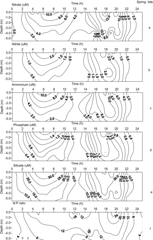
The water column was quasi-isothermal during the spring tide, with temperatures varying less than 1°C between surface and bottom layers (Fig. 5a). Alternation between vertical homogeneity and stratification conditions was the main characteristic of spring tide profiles of salinity and inorganic nutrients, closely related to the tidal phase. At flood slack-tide, the water column was isohaline and the ebb currents disrupted this homogeneity, carrying low salinity waters from the upper reaches, preferentially along the surface, resulting in transient ebb slack-tide stratification (Figs. 5b, 5c). Ebb currents were stronger than flood currents, reaching speeds as high as 0.8 and 1.0 m s-1 at the surface.
DOS levels (Table 1 and Fig. 5d) indicated the saturation and even the over-saturation of the saltier waters. This feature was due to the preponderance of coastal waters at the sampling site, and also to more intense currents, which favor the dissolving of oxygen in the water. The lower DOS values (< 70.0%) occurred in the slack ebb tide with the less saline water outflow.
A wider range of variation was observed in Zeu (between 1.4 and 6.8 m) as compared to the neap
tide. The lower values occurred mainly in the second cycle (Fig. 5e), related to the presence of higher TSS along the whole water column (Fig. 7c) and associated with higher current speeds. Maximum Zeu values were
detected in slack water periods.
The same structure observed for salinity also appeared in the distribution of nutrients, revealing a close relationship between brackish waters and nutrient availability (Figs. 6a to 6e). In the second cycle, ebb currents were stronger, promoting a more intense brackish water outflow, and higher nutrient concentrations were then observed.
Given that coastal water entrainment was stronger in spring tides, the average nutrient values under these conditions were lower than in neap tides, reflecting the lower nutrient levels in coastal water (Table 1). Silicate distribution showed the greatest contrast. Nitrate was again the main inorganic nitrogen form, but ammonium concentrations were almost as high as those of nitrate. N: P ratios were below 16:1 most of the time (Fig. 6f) with a mean value of 11.2 (Table 1) indicating nitrogen deficiency relative to the phosphate content.
Chl-a mean concentration was three-fold higher than that observed in the neap tides (Table 1). The increase was related to ebb currents and the higher Chl-a concentrations (Fig. 7a) occurred when the flux in the entire water column was seaward. The proportion of Chl-aact was around 50%, being slightly
higher in the surface than in the bottom waters. In the Chl-a maxima the Chl-aact percentage was low,
Fig. 5. Time-space distribution of hydrographic variables followed at the fixed station in Bertioga channel during the spring tide: (a) Temperature (°C), (b) Salinity, (c) u velocity component (m s-1), (d) % Dissolved Oxigen Saturation (DOS) and (e) Euphotic Zone Depth (Zeu, m). The dots in (a) represent the sampling points.
-8,0 -6,0 -4,0 -2,0 0,0
0 2 4 6 8 10 12 14 16 18 20 22 24
D
ept
h
(
m
)
Night period
0 2 4 6 8 10 12 14 16 18 20 22 24
Time (h)
-6.0 -5.0 -4.0 -3.0 -2.0 -1.0 0.0
De
p
th
(
h
)
0 2 4 6 8 10 12 14 16 18 20 22 24
Time (h)
-6.0 -5.0 -4.0 -3.0 -2.0 -1.0 0.0
D
ept
h
(
m
)
0 2 4 6 8 10 12 14 16 18 20 22 24
Time (h)
-6.0 -5.0 -4.0 -3.0 -2.0 -1.0 0.0
D
ept
h
(
m
)
Spring tide
Temperature (C)
Salinity
u (m/s)
0 2 4 6 8 10 12 14 16 18 20 22 24
Time (h)
-5.0 -4.0 -3.0 -2.0 -1.0 0.0
D
e
pt
h (
m
)
DOS (%)
d b a
Time (h)
c
Zeu
0 2 4 6 8 10 12 14 16 18 20 22 24 Time (h)
-5.0 -4.0 -3.0 -2.0 -1.0 0.0
Dep
th
(m)
Nitrate (uM) Spring tide
0 2 4 6 8 10 12 14 16 18 20 22 24 Time (h)
-5.0 -4.0 -3.0 -2.0 -1.0 0.0
De
p
th (
m
)
Nitrite (uM)
0 2 4 6 8 10 12 14 16 18 20 22 24 Time (h)
-5.0 -4.0 -3.0 -2.0 -1.0 0.0
Dep
th (m)
Ammonium (uM)
0 2 4 6 8 10 12 14 16 18 20 22 24 Time (h)
-5.0 -4.0 -3.0 -2.0 -1.0 0.0
Dept
h (m)
Phosphate (uM)
0 2 4 6 8 10 12 14 16 18 20 22 24 Time (h)
-5.0 -4.0 -3.0 -2.0 -1.0 0.0
Dep
th
(m)
Silicate (uM)
0 2 4 6 8 10 12 14 16 18 20 22 24 Time (h)
-5.0 -4.0 -3.0 -2.0 -1.0 0.0
Dep
th (m)
N:P ratio
a
b
c
d
e
f
Fig. 7. Time-space distribution of biological variables monitored at the fixed station in Bertioga channel during the spring tide: (a) Chl-a (mg m-3), (b) Chl-a
act (% of the total Chl-a) and (c) Total Suspended Solids (TSS, mg l-1). Transport
Time-space averages for each variable obtained from the data series at the fixed station both in neap and spring tides (Table 1) indicate that the overall nutrient content at the sampling site was higher in the neap tides. However, DO and Chl-a showed higher averages in the spring tide, revealing the relationship between these variables and the salt water inflow. These data denote the presence of a larger amount of brackish water at the fixed station site during the neap tide. The difference between the averages are related to the migration of the mixing zone within the fortnightly tidal cycle which plays an important role on transport balances.
Table 2 presents the results of the mean advective transport during two full tidal cycles of both neap and spring tides, focusing on the relative contribution of the seven main components to the total
transport computed for nutrients, TSS and Chl-a. The percentage error between the results given by equations 2 and 7 ranged from 0.4 to 15.7, indicating that the transport terms considered explained the larger part of the variation. All the properties studied were exported to the sea, except total Chl-a at neap tide, which was imported. Net transport of dissolved constituents (nutrients) was higher at the neap than at the spring tide, whereas particulate constituents were exported more intensively at spring tide.
In both tides, almost all the transport terms displayed an advective behavior. Freshwater discharge and tidal correlation were responsible for a significant contribution to total transport. In the neap tide, gravitational circulation and tidal correlation acted as dispersive terms for Chl-a, being responsible for its net importation. In the spring tide, gravitational circulation and oscillatory shear were important dispersive factors for Chl-a, Chl-aact and TSS.
Spring tide Chl-a (mg/m3)
0 2 4 6 8 10 12 14 16 18 20 22 24
Time (h)
-5.0 -4.0 -3.0 -2.0 -1.0 0.0
Dep
th (
m
)
Active Chl-a (%)
a
b
0 2 4 6 8 10 12 14 16 18 20 22 24
Time (h)
-5.0 -4.0 -3.0 -2.0 -1.0 0.0
De
pt
h
(m)
0 2 4 6 8 10 12 14 16 18 20 22 24
Time (h)
-5.0 -4.0 -3.0 -2.0 -1.0 0.0
Depth (m)
Tidal correlation represents the correlation between the mean values of velocity and salinity, being a non-zero value when the salinity maximum and minimum do not occur simultaneously with the slack flood and ebb tides, respectively, as indicated in figures 2c and 5c.
D
ISCUSSIONIn spite of the great influence of tidal currents in estuaries, most studies in estuarine environments deal mainly with the influence of the freshwater flux (Dyer, 1997). However, in the majority of coastal plain estuaries, tidal currents are the main source of energy for the mixture of freshwater and salt waters, resuspension and longitudinal transport of sediments (Nichols & Biggs, 1985). In a recent review, Uncles (2002) stated that, from a process viewpoint, much more attention is now being given to
interpreting intratidal behavior, including the effects of tidal straining and suspended fine sediment on water column stratification, stability and turbulence generation and dissipation. The results obtained in the BC indicate clearly that tides affect both the nutrient and Chl-a vertical distribution strongly. The differences between tidal phases are remarkable because brackish and coastal waters possess very distinctive characteristics, mainly related to nutrient content. According to Gianesella et al. (2000) the main source of nutrients to the channel is land drainage, especially in the upper reaches where the channel is surrounded by mangroves. The Itapanhaú River and ocean waters have a lower nutrient content than brackish waters and the mixture of these three waters, resulting especially from the spring tide, leads to an overall decrease of nutrients in the water column.
Table 2. Net transport results computed for nutrients, Chl-a, Chl-aact and TSS during neap and spring tides in the winter of 1991 at Bertioga channel (negative values mean importation and positive, exportation). Computations were done by equations 2 and 7 the percentual error between them is showed.
Neap Tide NO3-
(g m-1
s-1
) NO2-
(g m-1
s-1
) NH4+
(g m-1
s-1
) DIN (g m-1
s-1
) PO4-3
(g m-1
s-1
)
Si(OH)4
(g m-1
s-1
) Chl-a (mg m-1
s-1
) Chl-aact
(mg m-1
s-1
)
Freshwater discharge 0.112 0.011 0.025 0.144 0.018 0.515 0.212 0.092
Stokes velocity 0.018 0.002 0.003 0.023 0.003 0.083 0.034 0.015
Tidal correlation 0.090 0.015 0.032 0.137 0.018 0.116 -0.153 0.042
Gravitational circulation 0.037 0.001 0.009 0.047 -0.002 0.151 -0.158 -0.069
Oscillatory shear 0.021 0.002 0.005 0.028 0.004 0.062 0.038 0.033
Tidal dispersion 0.018 0.002 0.004 0.024 0.002 0.057 -0.035 -0.019
Residual circulation -0.002 0.000 0.000 -0.003 0.000 -0.007 0.004 0.002
Net transport (eq. 7) 0.295 0.033 0.073 0.401 0.042 0.977 -0.057 0.097
Net transport (eq. 2) 0.296 0.033 0.074 0.403 0.043 0.981 -0.068 0.088
Error (%) 0.4 0.5 1.2 0.5 0.8 0.4 15.7 9.5
Spring Tide NO3-
(g m-1
s-1
) NO2-
(g m-1
s-1
) NH4+
( g m-1
s-1
) DIN ( g m-1
s-1
) PO4-3
(g m-1
s-1
)
Si(OH)4
(g m-1
s-1
) Chl-a (mg m-1
s-1
) Chl-aact
(mg m-1
s-1
) TSS (g m-1
s-1
)
Freshwater discharge 0.071 0.01 0.017 0.098 0.016 0.386 0.699 0.348 7.389
Stokes velocity -0.024 -0.003 -0.006 -0.033 -0.006 -0.130 -0.236 -0.117 -2.490
Tidal correlation -0.001 0.017 0.020 0.035 0.019 0.305 0.749 0.124 13.190
Gravitational circulation 0.031 0.003 0.005 0.038 0.003 0.091 -0.177 -0.024 - 4.340
Oscillatory shear 0.019 0.005 0.008 0.032 0.006 0.091 -0.225 -0.113 -2.017
Tidal dispersion 0.001 0.000 0.000 0.001 0.000 0.009 -0.072 0.005 -1.597
Residual circulation -0.003 0.000 -0.001 -0.037 0.000 -0.011 -0.007 -0.003 -0.038
Net transport (eq. 7) 0.094 0.031 0.043 0.168 0.038 0.741 0.732 0.220 10.097
Net transport (eq. 2) 0.092 0.030 0.042 0.164 0.038 0.733 0.762 0.229 10.787
Eyre & Balls (1999) compared tropical and temperate estuaries and debated whether, regardless of estuaries from different regions having a number of unifying features, such as salinity gradients, tidal variations and terrestrial inputs, they also have a number of important differences. The most distinct ones are timing and variability of major physical forcing that may control biogeochemical processes along salinity gradients. The BC presents some of the typical tropical characteristics reported by those authors, such as high mean temperature with a wider variation along the salinity gradient (almost 4oC (Gianesella et al., 2000) against <1oC in temperate estuaries), high silicate content, high rainfall, lower annual range of light intensity and mangroves as the predominant intertidal vegetation.
Australian estuaries are more episodic than those of Europe or North America (Eyre et al., 1998) due to a highly variable flushing time over the year (<1 to 415 days). Flushing time controls the degree to which materials are processed as they pass through the estuary (Eyre & Twigg, 1997). The values calculated for the periods studied in the BC are of the order of 2.1-3.5 days (Miranda et al., 1998), a range similar to those observed in European and North American estuaries. Rendell et al. (1997) consider the low freshwater residence time (1-14 days) as responsible for generally low nutrient retention (N, P, Si) in the Great Ouse estuary (England). In BC, the renovation rates for each tidal cycle are of the order of 12.9% in the spring and 24.4% in the neap tides, favoring the exportation of the high nutrient load of the brackish water toward the estuary´s lower reaches and the adjacent sea. In fact, despite being surrounded by mangrove forest, considered as an efficient nutrient sink (Alongi, 1996), the BC displays higher mean values of inorganic nutrients (Table 1) than those presented by Eyre & Balls (1999) for tropical Australian estuaries.
When a larger area of the mangrove forest is flooded, due to the higher spring tidal elevation, the input of a larger amount of phosphate in solution from the mangrove interstitial waters is promoted, not completely removed from the soluble fraction by the adsorption to the extant particulate matter. In the BC phosphate and salinity correlate negatively at spring tide (R2= -0.68), indicating that the phosphate input occurs from brackish surface waters.
Webb and D´Elia (1979) have corroborated previous reports that the release of phosphate from sediment is enhanced at low oxygen tensions. They also ascertained that vertical mixing accompanying spring-tidal destratification promotes oxygen replenishment in deep water, allowing aerobic processes to proceed, and accelerates the input of benthos-regenerated nutrients into the euphotic zone.
In spring tide series, DOS correlated positively with salinity (R2=0.79) and negatively with PO
4-3 (R2
=-0.59). In this sense, the migration of the mixing zone along the estuary is an important forcing because DOS-rich salt waters favor oxygen replenishment to the benthos and the nutrient input continuity, especially in the upper reaches. Silicate concentrations also correlate negatively with salinity (R2=-0.83) in the spring tide and the maximum values are compatible with those reported by Eyre & Balls (1999) for tropical estuaries.
Brackish waters presented high N:P ratios, with a single case over 30, the limit above which phosphate limitation is characterized (Goldman et al., 1979; Dortch & Whitledge, 1992). This indicates that the BC maintains nutritional equilibrium without being eutrophicated, conversely to the adjacent heavily polluted Santos estuary (Moser et al., 2002), which displays N:P ratios of around 4 during winter (mean value of DIN= 72µM). A different situation is found in the Camboriú river estuary (Pereira Filho et al., 2001) where N:P ratios above 100 occur. This is a consequence of the input of N and P from the fertilizers used in agricultural activities in the neighboring areas, associated with a high adsorption of phosphorus by the particulate matter, resulting in an imbalance in the adjacent bay. Conversely, some tidal creeks of the Cananéia estuary (Southeastern Brazil) present very low ratios due to the extreme anoxic conditions which favor the decomposition of the organic matter stems from sulfate reduction (90% against 10% from iron reduction). This explains why the mangrove forest there does not export significant amounts of nitrogen into the adjacent lagoon (Carmouze et al., 1998). In the BC anoxic conditions were not detected, even in the upper reaches (Gianesella et al., 2000).
time prevents phytoplankton biomass accumulation inside the estuary.
Uncles (2002) ascertained that stratified periods of enhanced estuarine salt transport occurred at five-day intervals once a month during the apogean neap tides, corroborating the theoretical prediction of Bowen (1999 apud Uncles, 2002) who, by using numerical models and analysis, demonstrated that salt transport is increased dramatically during stratified periods when vertical mixing is weak. Actually, Miranda et al. (1998) computed higher net salt transport during neap tide (3.61 Kg m-1 s-1) than during spring tide (2.63 Kg m-1 s-1) in the BC. The
same pattern was observed in our values for inorganic nutrient transport, which nutrients were exported more intensely at neap tide as a consequence of a lower entrainment of the nutrients in the saltier water, given that the mixing zone was in the lower reaches related to the sampling point. At this time freshwater discharge and tidal correlation were the main routes of net transport.
The physical behavior of transport properties at a point in an estuary depends upon its position along the estuarine axis, freshwater input and tidal range, among other factors. Tidal propagation in the BC is a mixture of standing and progressive waves due to the dissipation of tidal energy by bottom friction, typical of a partially mixed estuary (Miranda et al., 1998). This bottom friction probably plays an important role in the suspension of the settled phytoplankton and epibenthic cells, shown by deep Chl-a and TSS peaks related to the maximum spring-ebb currents. This indicated a higher contribution of advective processes in the transport of these variables. This suggested the channel acted as a TSS exporter due to the residual seaward currents, corroborated by the seaward net transport computations of Chl-a and TSS for spring tides. Uncles et al. (1985) modeled the action of tidal currents on sediment suspension in a partially mixed estuary. They observed a large spring-neap tidal variation in suspended solid concentration due to the bed sediment resuspension in the faster spring peak currents, and that the tidal pumping of suspended sediments directed up-estuary by the spring tides probably contributed to the formation of the turbidity maximum. In the present study, the gravitational circulation was the most important term in the dispersive transport of TSS during the spring tide.
Stokes velocity represents the mass transport generated by tidal wave propagation in the estuary related to the bottom topography slope. Theoretically, this term corresponds to an exportation mechanism pushing materials down-estuary, favoring in this way the decrease of allochthonous substances discharged into the estuary (Miranda et al., 2002). However, in the BC this term was up-estuary in the spring tide, acting as a dispersive component for every property
studied, as was also observed for salt transport by Miranda et al. (1998), representing the third main parcel of the total transport. This discrepancy between theoretical and practical results may be due to the attenuation of the tidal wave in the Largo do Candinho, but it represents an important mechanism for the introduction of materials from coastal waters into the inner estuary.
Chl-a and Chl-aact were exported only in the
spring tide, when the input of ocean waters into the BC was greater, carrying phytoplankton into and out of the estuary. A more subtle effect of bottom friction on the resuspension of the settled senescent phytoplankton and also epibenthic cells occurred during the neap tide, when the currents were weak. In this case, Chl-aact was exported and total Chl-a was
imported, indicating that phaeophytin-rich cells remain in the estuary whereas the healthy phytoplankton (cells with a higher Chl-aact content) are
actually exported.
In terms of dissolved nutrients and Chl-a, the BC exports a higher load than the eutrophic Camboriú river estuary (Pereira Filho et al., 2001). These data illustrate the importance of the contribution of nutrients from the BC into the adjacent sea, in spite of the fact that this channel presents a low anthropogenic impact. It should also be remembered that this evaluation was conducted under the driest annual conditions and that probably the loads tend to increase in summertime due to the augment in land drainage.
The maturity of an estuarine system may be characterized according to the marsh-estuarine continuum hypothesis (Dame et al., 1992; Dame & Allen, 1996) which states that a mature ecosystem exports both particulate and dissolved material whereas immature systems import both constituents. During the winter dry season, the BC acted as a nutrient exporter under both tidal conditions and a chlorophyll importer during the neap tide, allowing this estuary to be classified as a middle-aged system, as it exports dissolved materials and occasionally imports particulate ones, considering the location of the study site and time interval used for the calculations.
estuarine upper reaches are amplified by this mechanism, especially in periods of low freshwater discharge. In this sense the knowledge of the behavior of each component of transport, related to a particular dynamic condition, provides information on the potential fragility of the ecosystem.
A
CKNOWLEDGEMENTSThe present work represents part of the results of an interdisciplinary investigation of the Bertioga channel supported by Marinas do Brasil Associados Ltda. / Fundação de Estudos e Pesquisas Aquáticas.
R
EFERENCESAlongi, D. M. 1996. The dynamics of benthic nutrient pools and fluxes in tropical mangrove forests. J. Mar. Res., 54:123-148.
Aminot, A. & Chaussepied, M. 1983 Manuel des analyses chimiques en milieu marin. Brest, C.N.E.X.O, 379p. APHA (American Public Health Association) 1985. Standard
methods for the examination of water and wastewater. Washington, APHA, 1268p.
Bowden, K. F. 1963. The mixing processes in a tidal estuary. Int. J. Air Water Pollut., 7:343-365.
Carmouze, J. P.; Gianesella-Galvão, S. M. F.; Nishihara, L. & Mesquita, H.S.L. de. 1998. Modeling chemical changes of tidal waters emerging from a mangrove forest at Cananéia, Brazil. Mangr. Salt Marshes, 2:43-49. DAEE (Departamento de Águas e Energia Elétrica) 2005.
(www.daee.sp.gov.br).
Dame, R. F. & Allen, D. M. 1996. Between estuaries and the sea. J. expl. Mar. Biol. Ecol., 200:169-185.
Dame, R. F.; Childers, D. & Koepfler, E. 1992. A geohydrologic continuum theory for the spatial and temporal evolution of marsh –estuarine ecosystems. Nether. J. Sea Res., 30:63-72.
Dortch, Q. & Whitledge, T. E. 1992. Does nitrogen or silicon limit phytoplankton production in the Mississipi river plume and nearby regions? Continent. Shelf Res., 12, 1293-1309.
Dyer, K. R. 1974. The Salt Balance in Stratified Estuaries. Estuar. coast. Mar. Sci., 2:273-281.
Dyer, K. R. 1997. Estuaries: a Physical Introduction. John Wiley, Chichester. 195 p.
Eyre, B. 1998. Transport, retention and transformation of material in Australian estuaries. Estuaries, 21(4):540-551.
Eyre, B. D. & Twigg, C. 1997. Nutrient behavior during post-flood recovery of the Richmond River estuary northern NSW, Australia. Estuar. coast. Mar. Sci., 44:311-326. Eyre, B. & Balls, P. 1999. A comparative study of nutrient
behavior along the salinity gradient of tropical and temperate estuaries. Estuaries, 22(2A):313-326.
Eyre, B., Hossain, S. & McKee, L. 1998. A suspended sediment budget for the modified subtropical Brisbane River Estuary, Australia. Estuar. coast. Mar. Sci., 47(4):513-522.
Gianesella, S. M. F.; Saldanha-Corrêa, F. M. P. & Teixeira, C. 2000. Tidal effects on nutrients and phytoplankton distribution in Bertioga Channel, São Paulo, Brazil. Aquat. Ecosys. HealthManag., 3:533-544.
Goldman, J. C.; McCarthy, J. J. & Peavey, D. G. 1979. Growth rate influence on the chemical composition of phytoplankton in oceanic waters. Nature, 279:210-215. Grasshoff, K.; Ehrhardt, M. & Kremling, K. 1983. Methods
of Seawater Analysis. Weinheim, Verlag Chemie. 419p. Hansen, D.V. & Rattray Jr, M. 1966. New dimensions in
estuarine classification. Limnol. Oceanogr., 11:319-326. Harari, J. & Camargo, R. 1997. Simulações da circulação de
maré na região costeira de Santos (SP) com modelo numérico hidrodinâmico. Pesq. Naval, 10:173-188. Holm-Hansen, O.; Lorenzen, C. J.; Holmes, R. W. &
Strickland, J. D. H. 1965. Fluorimetric determination of chlorophyll. J. Cons. perm. intern. Explor. mer,30:3-15. Hunkins, K. 1981. Salt dispersion in the Hudson Estuary. J.
Phys. Oceanogr., 11:729-738.
LOICZ program homepage (http://data.ecology.su.se/MNODE/).
Lucas, L. V.; Koseff, J. R.; Cloern, J. E.; Monismith, S. G. & Thompson, J. K. 1999a. Processes governing phytoplankton blooms in estuaries. I. The role of horizontal transport. Mar. Ecol. Prog. Ser., 187:1-15. Lucas, L. V.; Koseff, J. R.; Monismith, S. G.; Cloern, J. E. &
Thompson, J. K. 1999b. Processes governing phytoplankton blooms in estuaries. II. The role of horizontal transport. Mar. Ecol. Prog. Ser., 187:17-30. Miranda, L. B. de & Castro, B. M. 1996. On the salt
transport in the Cananéia sea during a spring tide experiment. Rev. bras. Oceanogr., 44(2):123-133. Miranda, L. B. de; Castro, B. M. & Kjerfve, B. 2002.
Princípios de Oceanografia Física de Estuários. São Paulo. EDUSP. 414 p.
Miranda, L. B. de; Castro, B. M. & Kjerfve, B. 1998. Circulation and mixing due to tidal forcing in the Bertioga Channel, São Paulo, Brazil. Estuaries, 21(2):204-214.
Moser, G. A .O.; Gianesella, S. M. F.; Barrera-Alba, J. .J.; Bérgamo, A. L.; Saldanha-Corrêa, F. M. P.; Miranda, L. B. de & Harari, J. 2005. Instantaneous transport of salt, nutrients, suspended matter and chlorophyll-a in the tropical estuarine system of Santos. Braz. J. Oceanogr., 53(3-4).
Nichols, M. M. & Biggs, R. B. 1985. Estuaries. In: Davies Jr, R. A., ed. Coastal Sedimentary Environments.New York, Springer-Verlag. p.77-173.
Officer, C. B. & Kester, D. R. 1991. On estimating the non-advective tidal exchanges and non-advective gravitational circulation exchanges in an estuary. Estuar. coast. Shelf Sci., 32: 99-103.
Pereira Filho, J.; Schettini, C. A. F.; Rörig, L. & Siegle, E. 2001. Intratidal variation and net transport of dissolved inorganic nutrients, POC and chlorophyll a in the Camboriú River estuary, Brazil. Estuar. coast. Shelf Sci., 53:249-257.
Poole, H. H. & Atkins, W. R. G. 1929. Photo-electric measurements of submarine illumination throughout the year. J. Mar. Biol.Ass. U. K.,16:297-324.
Robertson, A. I. & Blaber, S. J. M. 1992. Plankton, epibenthos and fish communities. In: Robertson, A. I. & Alongi, D. M., eds. Tropical Mangrove Ecosystems.
Washington, DC. American Geophysical Union, p. 173-224.
Schubel, J. R. & Kennedy, V. S. 1984. The estuary as a filter, an introduction. In: Kennedy, V. S., ed.The Estuary as a Filter. Florida, Academic Press, p.1-15.
Simpson, J. H.; Vennell, R. & Souza, A. J. 2001. The salt fluxes in a tidally-energetic estuary. Estuar. coast. Shelf Sci., 52:131-142.
Uncles, R. J. 2002. Estuarine Physical Processes Research, Some Recent Studies and Progress. Estuar. coast. Shelf Sci., 55:829-856.
Uncles, R. J.; Elliott, R. C. A. & Weston, S. A. 1985. Observed fluxes of water, salt and suspended sediment in a partly mixed estuary. Estuar. coast. Shelf Sci., 20:147-167.
UNESCO, 1973. International oceanographic tables. Tables of oxygen. National Institute of Oceanography of Great Britain and UNESCO 2.
UNESCO, 1981. Background papers and supporting data on the Practical Salinity Scale 1978. UNESCO Tech. Pap. Mar. Sci., 37:1-144.
Webb, K. L. & D´Elia, C. F. 1979. Nutrient and Oxygen Redistribution During a Spring Neap Tidal Cycle in a Temperature Estuary. Science 207:983-985.
Wollast, R. 1983. Interactions in estuaries and coastal waters. In: Bolin, B. & Cook, R. B. eds. The major biogeochemical cycles and their interactions. Paris, SCOPE. p.385-407.
Yentsch, C. S. & Menzel, D. W. 1963. A method for the determination of phytoplankton, chlorophyll and phaeophytin by fluorescence. Deep-Sea Res., 10:221-231.
Sources of Unpublished Material
Barrera-Alba, J. J.; Gianesella, S. M. F.; Harari, J.; Miranda, L. B.; Moser, G. A. O.; Nishihara, L.; Picarelli, S. S.; Saldanha-Corrêa, F. M. P.; Jakovac, A. C. C.; Ricci, F. P. & Mello, R. L. 2002. Transporte de ferro e silicato dissolvidos nas entradas do sistema estuarino-lagunar de Cananéia-Iguape, julho de 2001. In: Congresso Brasileiro de Pesquisas Ambientais, Anais. 2. Santos, 2002. p.1-5.
Moser, G. A. O.; Gianesella, S. M. F.; Cattena, C. O.; David, C. J.; Barrera-Alba, J. J.; Saldanha-Corrêa, F. M. P. & Braga, E. S. 2002. Influência das marés sobre o fitoplâncton no Sistema estuarino de São Vicente Santos. In: Congresso de Pesquisa Ambientais. Anais. 2, Santos, 2002. p.1-5.