The electrospinning of PA66 has been done by other authors8,9; Martin et al.8 electrospun solutions of PA66 in formic acid with 10 and 16 wt.(%)/v. They obtained non-woven mats with 0.06-2.80 µm of diameter. Tsai and Chen9 also electrospun solutions of PA66 in for-mic acid. They obtained nanofibers with average diameter of 78 nm. However, none of these works analyzed the influence of the PA66 molecular weight and terminal carboxylic and amines groups on the electrospinning.
On the other hand, polyamide 6 (PA6) has been more extensively studied. Hag-Yong et al.10 electrospun solutions of PA 6 in sulfuric acid with 15 wt.(%)/v, obtaining fibers with average diameters lower than 500 nm. Ryu et al.11 also electrospun solutions of PA6 in formic acid at 15 and 30 wt.(%)/v obtaining fibers with average diameters between 90 and 500 nm. Dersh et al.12 measured the Herman’s ori-entation function of electrospun fibers from formic acid solutions and concluded that γ crystals with high orientation along the flow direction formed the PA6 structure. Stephens et al.13 electrospun PA6 solutions in hexa-isofluoropropanol and found that the PA6 crystal-line structure changed from α-phase to γ-phase. Suphapol et al.14,15 electrospun solutions of PA6/formic acid with different molecular weights; they found that the higher the molecular weight, the higher the nanofibers average diameters.
The addition of an ionic salt sometimes increases the electrical conductivity of the solution. As Reneker et al.3 pointed out, in an uncharged ionic solution, there is the same number of positive and negative ions in each volume element. When an external electrical
1. Introduction
Electrospinning of polymer solutions has been extensively used in the last years to produce polymeric fibers of nano-dimensions1-6. New companies based on this process, like eSpin Technologies, Nanotechnics and Kato Tech emerged in the last years while com-panies like Donaldson and Freudenberg have been using electrospun fibers for the last two decades7. In the electrospinning process, the polymeric solution is put in a capillary tube or syringe and a metallic electrode, connected to a grounded high voltage supply is immersed in the polymeric solution. An electrical tension is applied and when the electrostatic forces overcome the solution’s surface tension, the hemispherical surface of the capillary’s drop (Taylor’s cone) elongates and an electrically charged jet of polymeric solution is generated. During the jet’s trajectory to the collector, the solvent evaporates; thus solid nanofibers are formed and collected in the form of non-woven mats on the metallic collector. The variables of this process are many: solutions concentration (which determines the solutions viscosity), solvent type, applied electrical field, ionic salts addition (which can increase the solution’s electrical conductivity), flow rate, temperature and others.
The molecular weight, the distribution of molecular weight and branching of the polymer have also influence on the electrospinning because can interfere on the solvent’s evaporation rate, crystalliza-tion kinetics and solucrystalliza-tions viscosity. In the case of poly-condensacrystalliza-tion polymers like PA66, the amount of terminal carboxylic and amines groups should also have an effect on the process.
Electrospinning and Characterization of Polyamide 66
Nanofibers With Different Molecular Weights
Lilia Muller Guerrinia, Marcia Cristina Brancifortia, Thomas Canovab, Rosario Elida Suman Bretasa*
a
Department of Materials Engineering, Federal University of São Carlos,
13565-905 São Carlos - SP, Brazil
b
Rhodia Têxtil, Santo André - SP, Brazil
Received: December 23, 2008; Revised: May 8, 2009
Polyamide 66 (PA66) nanofibers of different molecular weights were obtained by electrospinning of formic acid solutions. An ionic salt, NaCl, was also added to the solutions to increase the conductivity. PA66 concentrations between 15-17 wt.(%)/v and electrical fields between 2.0 and 2.5 kV/cm were the best conditions to produce the smallest nanofibers; however, the addition of NaCl increased the fibers average diameters.
The characterization of the fibers was done by scanning electron microscopy (SEM), differential scanning calorimetry (DSC), wide angle X rays diffraction (WAXD) and Fourier Transformed Infrared (FTIR). As the molecular weight decreased, the nanofibers average diameters also decreased; however, critical number average and weight average molecular weights were necessary for electrospinning. As the amounts of carboxyl terminal groups (CTG) increased, the nanofibers average diameters decreased; however, above CTG’s critical values of 8.7 x 10⁻⁵ mol.g–1 no electrospinning was possible. The addition of ionic salt increased the electrical conductivity
of the solutions and increased the nanofibers’ average diameters. By DSC, residual solvent in all the electrospun mats was found; two melting endotherms, one between 248 and 258 °C and the other one between 258 and 267 °C, depending on the sample were also observed. These endotherms were attributed to the melting, re-crystallization and re-melting of the PA66 α-phase. The nanofibers had low % of crystallinity compared to a textile fiber. By WAXS and FTIR, confirmation of the presence of α-phase crystals, of small dimensions and highly imperfect and of a very small amount of β and γ-phases crystals in the nanofibers structure was obtained.
Keywords: polyamide 66, electrospinning, nanofiber, characterization
CTG (v v ) f m
0
= − c (1)
where v = consumed volume of titration agent during the polyamide titration (l); v0 = consumed volume of titration agent in the white (without polyamide) titration (l); M = molarity of the titrate (mol.L–1); fc = correction factor of the titrate (calculated in a daily basis to correct possible errors in the titrate preparation); and m = sample mass (g).
The correction factor fc was determined by weighting a standard sample of pure potassium hydrogen phthalate. This standard sample was titrated with potassium hydroxide/glycol (0.1 N) solution. The correction factor was calculated using the following Equation 2:
fc = 1000 mfs / (V N 204.23) (2)
where mfs = mass of potassium hydrogen phthalate (g); V = volume of titrate (l); N = normality of the titrate; and 204.23 = equivalent-gram of potassium hydrogen phthalate.
The amount of amines terminal groups, ATG, was determined by potentiometer titration using phenol and tri-(hydroxy-methyl) amino methane as solvents of the polyamide at 40 °C and HCl as titration agent, in a potentiometer from Mettler Toledo®, model DL-50 with a Pt electrode. The ATG, in g.mol–1, was calculated using Equation 3:
ATG (v v )Mf m
0 c
= − (3)
The amount of humidity in the polyamide was determined by loss weight at 105 °C during 30 minutes in a vacuum oven.
The number average molecular weight, Mn, was determined from Equation 4:
M
ATG CTG
n= + +
∑
2 10 8 6 x
( ) (4)
where: 8 = number of end-chain groups that are neither amines or carboxyl groups19,20.
2.3. Solutions preparation and characterization
The polyamide 66/formic acid solutions were prepared at 40 °C, under agitation. The polyamide concentrations in the formic acid were 10, 15, 17 and 20 wt.(%)/v. Solutions with 1 wt.(%)/v of NaCl were also prepared.
The solutions electrical conductivities were measured in a conductimeter from Digimed®, model DM-31, with a Pt electrode. The solutions’ surface tension was measured by the du Nöy method using a tension meter from Krüss, model K6, with a Pt ring. The shear viscosity of the solutions at low shear rates was measured in an ARES rheometer, from Rheometrics Scientific, using Couette geometry with a gap of 2 mm between the cylinders, under nitrogen atmosphere, at 25 °C.
field is applied to the solution, the positive and negative ions move toward the negative and positive electrodes, respectively. The dif-ference in the number of positive and negative ions in a particular region (for example near the electrodes) is called the excess charge. The excess charge produces an electrical field that extends for large distances. When an ionic salt is added, it dissociates into equal numbers of positive and negative ions, which increase the electrical conductivity of the solution by increasing the number of ions per unit volume, but do not increase the excess charge. Thus, for each polymeric solution there is a suitable ionic salt which will increase the electrical conductivity depending on the initial excess charge. For example, studies of the effect of the addition of NaCl in poly (vinyl alcohol) electrospun solutions16 have shown that the fibers average diameters decrease when the ionic salt is added; however, other studies in electrospun solutions of PA6/formic acid/NaCl14 have observed that the fibers’ average diameter increase when the salt is added. Even no effect on the fibers average diameters17 has been found.
Thus, in this work, the influence of the molecular weight and amount of terminal carboxylic and amines groups on the average diameters of electrospun nanofibers of PA66 will be investigated. The influence of the addition of an ionic salt on these fibers average diameters will also be studied.
2. Experimental
2.1. Materials
Two different molecular weights PA66 from Rhodia® were used, sample B and sample C. Sample B was post-condensed to obtain higher molecular weights, by two different routes in a vacuum oven: one at 140 °C, during 4 hours (sample A) and the other at 150 °C, during 24 hours (sample D). Sample C, suitable for the production of textiles, was also post-condensed by two different routes: one, before melt spinning, under vacuum, at 150 °C, during 24 hours (sample R) and the other during the liquid synthesis before melt spinning for 5 minutes (sample F)18.
The solvent used for the electrospinning solutions was formic acid (85%, from Synth®) with density of 1.22 g.mL–1 at 20 °C, molar mass of 46.03 g.mol–1, boiling point of 101 °C and melting point of 8.6 °C. Two conductive solutions (samples DS and RS) were prepared by the addition of NaCl (1 wt.(%)/v). Table 1 describes the nomenclature of the samples.
2.2. Polyamide 66 characterization
The amount of carboxyl terminal groups, CTG, was determined by titration using benzyl alcohol, phenolphthalein and methanol as solvents of the polyamide at 200 °C and a solution (0.1 N) of potas-sium hydroxide/glycol as titration agents. The CTG in g.mol–1 was calculated using the following Equation 1:
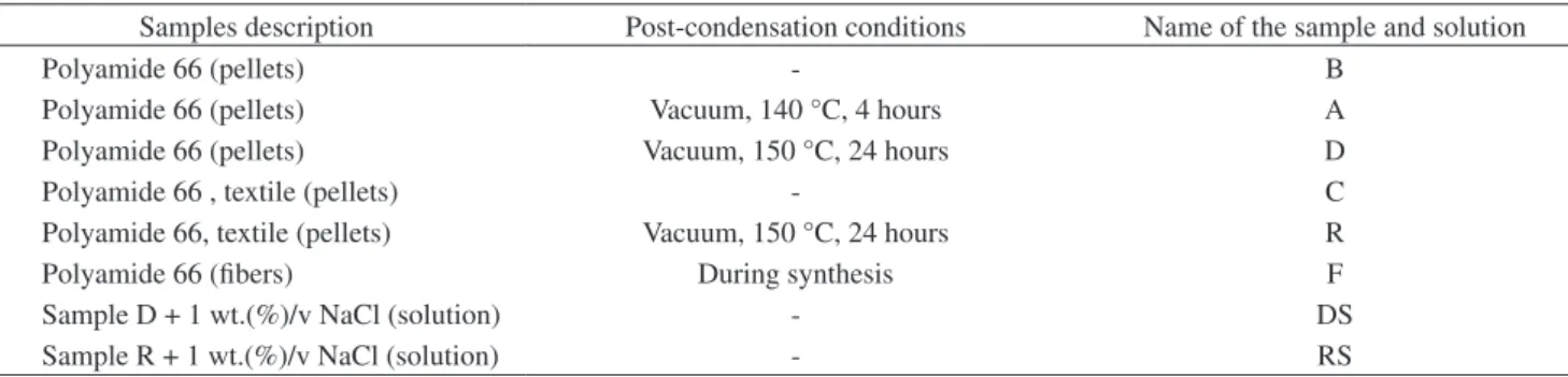
Table 1. Nomenclature of the polyamide 66 samples.
Samples description Post-condensation conditions Name of the sample and solution
Polyamide 66 (pellets) - B
Polyamide 66 (pellets) Vacuum, 140 °C, 4 hours A
Polyamide 66 (pellets) Vacuum, 150 °C, 24 hours D
Polyamide 66 , textile (pellets) - C
Polyamide 66, textile (pellets) Vacuum, 150 °C, 24 hours R
Polyamide 66 (fibers) During synthesis F
Sample D + 1 wt.(%)/v NaCl (solution) - DS
model XL30 FEG, operating at 30 kV. The number average diameter of the nanofibers and its distribution were calculated using the Image Pro-Plus software, in the Zeiss® micrographs; 100-120 fibers average diameters were measured.
2.5.2. Differential Scanning Calorimetry (DSC)
The glass transition temperature (Tg), the melting temperature (Tm), the amount of residual solvent (Xr.s) and the apparent amount of crystallinity of the nanofibers were measured by DSC, in a TA Instruments equipment, model Q100. The nanofibers were heated between 30 and 300 °C at 10 °C/min. The amount of crystallinity was calculated as the ratio between the melting enthalpy of the sample and the melting enthalpy of a theoretical 100% crystalline sample (∆Hfo
m). For the polyamide 66, ∆Hfom = 206 J.g–1 (21).
2.4. Solutions electrospinning
The electrospinning equipment was composed of a glass syringe (20 mL), a cylindrical collector and a high voltage supply, as shown in Figure 1. The syringe had Hamilton type stainless steel needles. The syringe electrode was a Cu thread sustained by a Cu peg. The collector was composed of a poly (vinyl chloride) tube (20 cm di-ameter), in which two wood disks were fixed at the ends. One of the wood disks was grounded, while the other was coupled to a motor, from Tekno®, model MRT910, with a velocity regulator, also from Tekno, model CVET2002. To measure the amount of rpm, a tachom-eter from Minipa®, model MDT-2238A was used. The collector was covered with an aluminum foil. The high voltage supply was from Bertan, model 210-30R.
The solutions electrospinning was done at room temperature and without room humidity control.
Tables 2 to 5 show the electrospinning conditions in which each sample was processed. Sample B was also electrospun, but no na-nofibers were formed at any condition.
2.5. Nanofibers characterization
2.5.1. Scanning Electron Microscopy (SEM)
The electrospun nanofibers were deposited on a double-face carbon adhesive and glued to the sample holder; silver paint was then added at the mats borders. The sample was gold sputtered and analyzed using two scanning electron microscopes: one from Zeiss®, Model DSM940, operating at 15 kV and the other from Phillips®,
Figure 1. Electrospinning set-up used in this work.
Table 2. Electrospinning conditions of sample A. Sample Solution concentration
(wt.(%)/v)
Electrical field (kV/cm)
Number average diameter (nm)
A3 10 2.5
-A4 10 2.9
-A5 15 2.0 131
A6 15 2.5 153
A13 17 2.0 148
A14 17 2.5 143
A2 17 2.5 155
A8 20 2.5 176
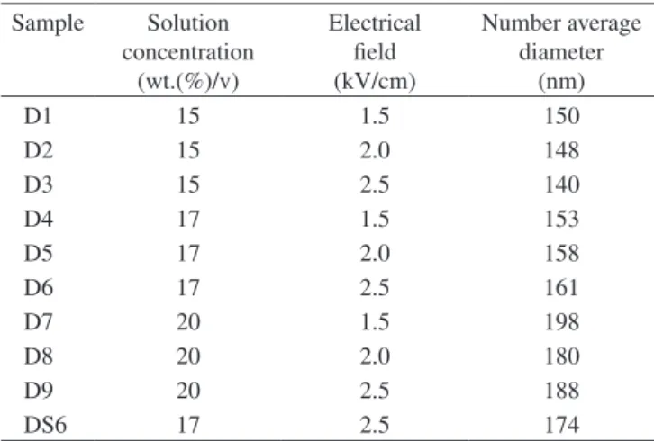
Table 3. Electrospinning conditions of sample D. Sample Solution
concentration (wt.(%)/v)
Electrical field (kV/cm)
Number average diameter
(nm)
D1 15 1.5 150
D2 15 2.0 148
D3 15 2.5 140
D4 17 1.5 153
D5 17 2.0 158
D6 17 2.5 161
D7 20 1.5 198
D8 20 2.0 180
D9 20 2.5 188
DS6 17 2.5 174
Table 4. Electrospinning conditions of sample R.
Sample Solution
concentration (wt.(%)/v)
Electrical field (kV/cm)
Number average diameter
(nm)
R1 15 1.5 150
R2 15 2.0 133
R3 15 2.5 117
R4 17 1.5 155
R5 17 2.0 136
R6 17 2.5 147
R7 20 1.5 185
R8 20 2.0 171
R9 20 2.5 163
RS1 15 1.5 163
RS2 15 2.0 152
RS3 15 2.5 152
RS4 17 1.5 158
RS5 17 2.0 184
RS6 17 2.5 166
RS7 20 1.5 182
RS8 20 2.0 179
probably due to the lower amount of amines and carboxyl groups (lower interactions).
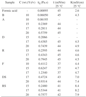
The addition of 1wt.%/v NaCl increased the electrical conduc-tivity of the solutions, as expected, but did not have any effect on the surface tension (Table 7). Solutions DS (7.0-7.4 mS/cm) and RS (7.9-8.4 mS/cm) almost doubled their conductivities by the addition of the salt, while the D and R solutions without salt had electrical conductivities between 4.5 and 4.9 and 4.5 and 4.6 mS/cm, respec-tively.
3.2. Nanofibers characterization
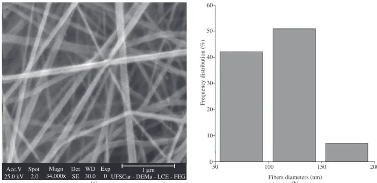
Some of the Phillips® scanning electron micrographs of the na-nofibers mats are shown in Figures 2, 3, 4, 5, 6 and 7, together with the distribution of nanofibers diameters calculated from the Zeiss® micrographs, as described in the experimental section. Tables 2 to 5 also show the number-average fiber diameter of all the electrospun samples. SEM micrographs of solution B are not shown, because, as said before, the electrospinning of that solution did not produce nanofibers, only drops.
2.5.3. Wide angle X ray diffraction (WAXD) and Fourier
Transform Infrared (FTIR)
To analyze the type of crystalline phases in the nanofibers, WAXD and FTIR experiments were done. The WAXD measurements were made in a diffractometer from Siemens® model D5005, operating with CuKα radiation, Ni filter, at 40 kV and 40 mA. The diffractograms were decomposed using the Origin 7.0 software with a Gaussian ap-proximation. For the infrared analyses, mats of the nanofibers were pile up to form a “film”. A FTIR equipment from Perkin Elmer® model Spectrum® 1000 was used, between 400 to 4,000 cm–1, in the transmission mode, with 4 cm–1 of resolution.
3. Results and Discussion
3.1. Polyamide 66 and solutions characterization
Table 6 shows the molecular weights, the ATG and the CTG of the different samples. As the molecular weight of the polyamide 66 increased as a consequence of post-condensation, the amount of amines and carboxyl terminal groups decreased, as expected. Sam-ple B had the lowest molecular weight, while samSam-ple F had the highest molecular weight.
Table 7 shows the zero shear viscosity, ηo, the surface tension τ and the electrical conductivity K of some of the solutions. The ηo of all the solutions increased with the increase in PA 66 concentrations, as expected. The values of surface tension and electrical conductivity of solutions A, D and R were similar to the values of PA6/ formic acid solutions. Li et al.22, for example, found surface tension values between 41 and 42 mN/m and electrical conductivities values between 4.6 and 4.3 mS/cm for PA6/formic acid solutions, with concentrations of 15 and 20 wt.(%)/v. Suphapol et al.15 also found surface tension values between 44 and 42 mN/m for the same type of solutions. The surface tension of solutions F was lower than of the other solutions, Table 5. Electrospinning conditions of sample F.
Sample Solution concentration (wt.(%)/v) Electrical field (kV/cm) Number average diameter (nm)
F2 10 1.5
-F3 10 2.0
-F8 15 1.0 164
F9 15 1.3 173
F5 15 1.5 150
F10 15 1.7 172
F6 15 2.0 140
F7 15 2.5 166
F21 15 3.0
-F15 17 1.0 176
F16 17 1.3 167
F14 17 1.5 165
F17 17 1.7 163
F12 17 2.0 170
F13 17 2.5 140
F18 17 3.0 182
F19 17 4.0 190
F20 17 5.0 187
Table 6. Properties of the polyamide 66.
Sample Mn
(g.mol–1)
Mw (g.mol–1)
ATG
x10–5 (mol.g–1)
CTG
x10–5 (mol.g–1)
B 13879 27759 4.78 8.83
A 14970 29940 4.02 8.54
D 17621 35242 2.80 7.76
R 16750 33501 2.43 8.71
F 19194 38388 1.70 7.92
Table 7. Zero shear viscosity, η0, surface tension, τ, and electrical conductivity, K, of the polyamide 66 solutions.
Sample C (wt.(%)/v) η0 (Pa.s) τ (mN/m) 25 °C
K(mS/cm) 25 °C
Formic acid - 0.00095 45 2.6
B 10 0.06050 45 4.3
A 10 0.06195 -
-15 0.2369 44
-17 0.2811 44
-20 0.5759 45
-D 15 0.2066 -
-17 0.4385 45 4.5
20 0.7439 44 4.9
R 15 0.2595 44 4.6
17 0.4343 45 4.6
20 0.7945 45 4.5
F 10 0.4112 37 4.4
15 0.6247 37 4.7
17 1.2340 37 4.7
DS 17 0.4724 43 7.0
20 0.9314 44 7.4
RS 15 0.2480 41 8.4
17 0.5344 41 8.2
(15 wt.(%)/v, 2.5 kV/cm) also produced the smallest average diameters of samples R. F6 (15 wt.(%)/v, 2.0 kV/cm) and F13 (17 wt.(%)/v, 2.5 kV/cm) conditions produced the smallest average diameters of samples F. In this last case, however, the F6 condition produced 79% of fibers with average diameter of 125 nm, while the F13 condition produced 47% of nanofibers with average diameter of 125 nm.
Therefore, PA66 concentrations in formic acid between 15-17 wt.%/v and electrical fields between 2.0 and 2.5 kV/cm were the best electrospinning conditions to produce the smallest nanofibers.
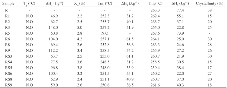
The addition of NaCl to sample R increased the nanofibers’ average diameters; the smallest diameter after the salt addition was obtained from the electrospinning of sample RS2 (15 wt.(%)/v, The smallest diameter (117 nm) was obtained from the
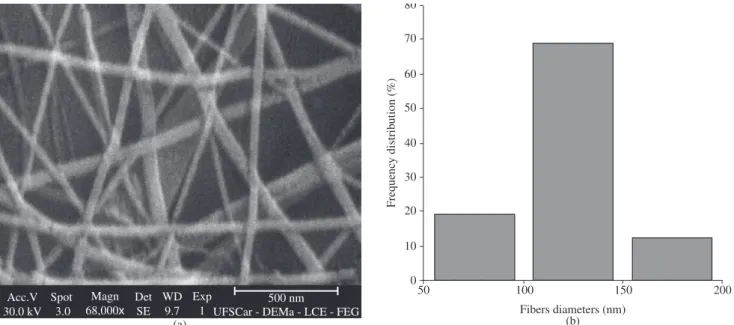
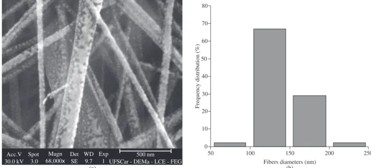
elec-trospinning of sample R, followed by sample A (131 nm), while samples D and F produced the largest fibers (140 nm). Therefore, as a rule, as the molecular weight increased, the nanofibers average diameters also increased; also, the higher the amount of carboxyl terminal groups, however, the lower the nanofibers average diameters. This last effect can be credited to the formation of hydrogen bonds that would facilitate the alignment of the macromolecules during the spinning.
The smallest average diameters of samples A were obtained at A5 electrospinning conditions (15 wt.(%)/v, 2.0 kV/cm); D3 conditions (15 wt.(%)/v, 2.5 kV/cm) produced the smallest av-erage diameters of samples D. R3 electrospinning conditions
Figure 2. a) Micrograph of sample A5 (Phillips® SEM); and b) diameter distribution (Zeiss® SEM).
combination allowed a quicker jet formation and higher amount of entanglements, producing fibers with lower average diameters.
Evaluating these results and the properties of the polyamide 66 (Table 6) it can be observed that the nanofibers average diam-eters is low when the polyamide 66 molecular weight decreases; however, critical molecular weights of Mn ≥ 14,970 g.mol–1 and Mw ≥ 29,940 g.mol–1 were necessary for electrospinning. In ad-dition, the nanofibers average diameter was low as the amount of carboxyl terminal groups (CTG) increased; however, above a critical CTG ≥ 8.7 x 10⁻⁵ mol.g–1 no electrospinning was possible.
Finally, to analyze the influence of the electrical field, a solution concentration of 15 wt.(%)/v was chosen. Samples D and R behaved as expected: the higher the applied electrical field, the lower the 2.0 kV/cm). The same average diameter increase was observed with
the addition of the salt to sample D; in this case, only condition DS6 (17 wt.(%)/v, 2.5 kV/cm) produced nanofibers. Thus, as a rule, the addition of NaCl increased the nanofibers’ average diameters.
To analyze the influence of concentration of the PA 66 solution, an electrical field of 2.5 kV/cm was chosen for comparison. Regarding samples A, D and R, it is observed that as the PA66 concentration in the solution increased, the nanofibers’ average diameter also in-creased. However, the opposite behavior is observed with sample F: the higher the PA66 concentration in the solution, the lower the na-nofibers average diameters. As said before, Sample F had the lowest surface tension but the higher Mn and Mw of all the samples; this
Figure 4. a) Micrograph of sample R3 (Phillips® SEM); and b) diameter distribution (Zeiss® SEM).
observed. That is, after the electrospinning residual solvent remained in the mats. The percentage of residual solvent Xr.s, was calculated from Equation 5:
X = m
m 100
r.s
T x (5)
where: m = vaporized formic acid mass (Kg); mT = DSC sample mass (Kg).
The vaporized formic acid mass was calculated from the DSC enthalpy of vaporization ∆Hv = m (c∆T + L), where ∆T = end va-porization temperature - initial vava-porization temperature, c = specific nanofibers average diameter. On the other hand, sample A had an
op-posite behavior: the higher the electrical field, the higher the average diameter. Sample F did not suffered influence of the increase of the electrical field, probably because it had the lowest surface tension of all the solutions.
Because the smallest nanofibers were obtained from sample R, only these mats were characterized by DSC. Figure 8 shows the heating runs of those mats, while Table 8 shows the main thermal transitions.
PA66 has a Tg between 45-65 °C. During the heating run, the Tg was not observed in the samples. Instead a large endothermic peak, ∆Hv (between 31 and 130 °C, accounted for solvent evaporation) was
Figure 6. a) Micrograph of sample RS2 (Phillips® SEM); and b) diameter distribution (Zeiss® SEM).
% crystallinity = (∆H1/∆Hfo
m) x 100 (6)
The apparent amount of crystallinity of both types of mats was between 15 and 30%. A textile PA66 fiber usually has around 40% of crystallinity23; that is, the nanofibers had low amount of crystallinity compared to a textile fiber.
The PA66 electrospinning occurred at room temperature; there-fore, it would be expected that no crystallization would occur during the spinning. However, two factors could have triggered crystal-lization: the lowering of the Tg by the solvent and the easiness of alignment of the PA66 macromolecules to form strong intermolecular hydrogen bonds.
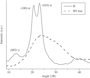
Figure 9 shows the diffractogram of sample R and one of the mats, R9. It can be observed that the crystal structure of sample R is pre-dominantly composed of α-phase, with diffraction peaks at 2θ = 20.5 and 23.0°[24,25]. A diffraction peak at 12.9° is also observed, related to the diffraction of γ-phase, as already found by Sengupta et al.24 in solutions of polyamide 66 with formic acid. On the other hand, heat capacity of the formic acid in the liquid state = 2169 J.kg–1 K and
L = latent heat of vaporization of formic acid = 41.4 x 10⁶ J.kg–1 [21].
The amount of residual solvent varied from 2.2 to 5.0% for the R mats without salt and from 2.4 to 3.8% for the R mats with salt.
Regarding the melting of the samples, it was observed that all samples had two melting endotherms: one between 248 and 258 °C, ∆H1, and the other one between 258 and 267 °C, ∆H2, depending on each sample. Because no cold crystallization was observed during the heating run, it was assumed that melting, re-crystallization and re-melting of the PA66 α-phase gave rise to these two endotherms. ∆H1 was attributed to the melting of imperfect α-crystals, which re-crystallized into more perfect α-crystals; these last ones, by its turn, melted absorbing the heat ∆H2. That is, electrospinning of PA 66 gave rise to the formation of imperfect α-crystals which melted between 248-258 °C.
Thus, the apparent % of crystallinity of the nanofibers was calculated as:
Figure 8. DSC heating run of sample R: a) R mats without salt; and b) R mats with salt.
Table 8. Main thermal transitions, amount of residual solvent, Xr.s, and crystallinity of sample R nanofibers. Sample Tg (°C) ∆Hv (J.g–1) X
r,s(%) Tm1 (°C) ∆H1 (J.g–1) Tm2 (°C) ∆H2 (J.g–1) Crystallinity (%)
R - - - 263.3 77.4 38
R1 N.O 46.9 2.2 252.3 31.7 262.4 55.1 15
R2 N.O 62.7 2.5 253.7 40.1 263.7 37.1 20
R3 N.O 148.0 5.0 257.2 51.9 265.0 22.8 25
R5 N.O 60.8 2.8 N.O - 267.6 73.9
-R6 N.O 104.0 4.2 257.1 61.5 264.1 25.0 30
R8 N.O 69.4 2.6 252.8 56.6 263.3 24.6 28
R9 N.O 112.2 3.4 258.5 54.2 265.9 27.2 26
RS3 N.O 63.7 2.5 255.0 61.1 260.7 21.9 30
RS4 N.O 77.5 3.6 248.5 31.2 258.5 30.5 15
RS5 N.O 96.8 3.8 248.0 33.9 259.4 38.4 17
RS6 N.O 100.4 3.2 251.5 55.1 260.2 22.0 27
RS8 N.O 62.9 2.4 251.1 40.9 260.7 37.0 20
RS9 N.O 59.0 2.6 250.6 36.5 261.6 40.3 18
4. Conclusions
The thermal and structural characterizations of the PA66 nanofib-ers allowed concluding that:
i) The lower the molecular weight, the lower the nanofibers average diameters; however, critical molecular weights of Mn ≥ 14,970 g.mol–1 and Mw ≥ 29,940 g.mol–1 were neces-sary for electrospinning.
ii) The higher the amount of carboxyl terminal groups, the lower the nanofibers average diameters; however, above critical CTG ≥ 8.7 x 10⁻⁵ mol.g–1 no electrospinning was possible.
iii) Polyamide 66 concentrations in formic acid between 15-17 wt.%/v and electrical fields between 2.0 and 2.5 kV/cm were the best conditions to produce the smallest nanofibers. iv) The addition of 1 wt.(%)/v NaCl doubled the electrical
conductivity of the solutions and increased the nanofibers’ average diameters.
v) The amount of residual solvent varied from 2.2 to 5.0% for the mats without salt and from 2.4 to 3.8% for the mats with salt; that is, all the mats contained residual solvent. All na-nofibers had two melting endotherms: one between 248 and 258 °C and the other one between 258 and 267 °C, depending on the sample. Because no cold crystallization was observed during the DSC heating run, it was assumed that melting, re-crystallization and re-melting of the PA66 α-phase gave rise to these two endotherms. The nanofibers had low % of crystallinity compared to a textile fiber. By WAXD and FTIR, confirmation of the presence of α-phase crystals, of small dimensions and highly imperfect and of a very small amount of β and γ-phase crystals in the nanofibers structure was observed. That is, electrospinning of PA66 produced nanofibers with imperfect and small α-crystals which melted between 248-258 °C.
Acknowledgements
The authors would like to thank Prof. D. F. Petri for the tension surface measurements, L. R. B. Santos for the electrical conductiv-ity measurements and Prof. R. Gregorio Filho for the high voltage power supply. This research was financially supported by CNPq and FAPESP.
the mats diffraction is large and amorphous-like, and no distinction between the diffraction of the crystalline planes and the amorphous halo is possible, indicating that the mats crystals are small and im-perfect, as also inferred from the DSC analysis.
Infrared analyses of the R samples were also done. Figure 10 shows the FTIR spectra of sample R and the R9 mat. Table 9 shows the main peaks found in both spectra. The α-phase is predominant in both samples (peaks at 2935 and 2934 cm–1); however, β and γ-phases (1437 and 1432 cm–1) are also observed, but in a very small concentration. The amorphous phase (922 and 1128-1136 cm–1) was not observed, probably due to overlapping by the crystalline peaks. The presence of CO2 (doublet at 2362 and 2336 cm–1, weak peak at 667 cm–1) and water vapor (~3400 and 1620 cm–1) was also observed.
Therefore the FTIR analyses confirmed the presence of mainly α-phase and small amounts of β and γ-phases in the PA66 nanofibers, as also found by Li et al.26 after electrospinning PA66 in tetrafluor-oethylene, TFE.
Figure 9. Diffractograms of sample R and R9 mat.
fiber diameter. Journal of Polymer Science: Part B: Polymer Physics.
2005; 43(24):3699-3712.
15. Supaphol P, Mit-uppatham C, Nithitanakul M. Ultrafine electrospun polyamide-6 fibers: effect of solvent system and emmiting electrode polarity on morphology and fiber average diameter. Macromolecular Materials and Engineering. 2005; 290(9):933-942.
16. Zhang C, Yuan X, Wu L, Han Y, Sheng J. Study on morphology of electrospun poly(vinyl alcohol) mats. European Polymer Journal. 2005; 41(3):423-431.
17. Demir MM, Yigor I, Yilgor E, Erman B. Electrospinning of polyurethane fibers. Polymer. 2002; 43(11):3303-3309.
18. Guerrini LM, Canova T, Bretas RES. Procede dobtention dun produit contenant des nanofibres et produit contenant des nanofibres. Fr Patent 0700053; 2007.
19. Russell SA, Robertson DG, Lee JH, Ogunnaike BA. Control of Product Quality for Batch Nylon 6,6 Autoclaves. Chemical Engineering Science.
1998; 53(21): 3685-3702.
20. Waltz JE, Taylor GB. Determination of the molecular weight of nylon.
Journal of Applied and Polymer Science. 1947; 19(1):448-450.
21. Lide DR. CRC Handbook of Chemistry and Physics. 88 ed. Taylor & Francis LLC, London: Editors Lide; 2007.
22. Li L, Bellan LM, Craighead HG, Frey MW. Formation and properties of nylon-6 and nylon-6/montmorillonite composite nanofibers. Polymer.
2006; 47(17):6208-6217.
23. Asprino TF. Avaliação do comportamento de fadiga da interface entre cordonéis de poliamida 66 compatibilizados com resorcinol formaldeido/ látex e compostos elastoméricos. [Master thesis]. São Carlos: Federal University of São Carlos; 2007.
24. Sengupta R, Tikku VK, Somani AK, Chaki TK, Bhowimick AK. Electron beam irradiated polyamide-66 films-I: characterization by wide angle X-ray scattering and infrared spectroscopy. Radiation Physics and Chemistry. 2005; 72(5):625-633.
25. Muellerleile JT, Freeman JJ. Effect of solvent precipitation on the cystrallization behavior and morphology of nylon 66. Journal of Applied Polymer Science. 1994; 54(22):135-152.
26. Li Y, Huang Z, Lü Y. Electrospinning of nylon-66-6,10-10 terpolymer.
European Polymer Journal. 2006; 42(7):1696-1704.
References
1. Huang ZM, Zhang YZ, KotakiM, Ramakrishna S. A review on polymer nanofibers by electrospinning and their applications in nanocomposites.
Composites Science and Technology. 2003; 63(15):2223-2253. 2. Ávila JPC. Alerta Tecnológico: Pedidos de Patentes sobre Nanotecnologia.
Available from: <http://pt.espacenet.com>. Access in: 18/05/2009. 3. Reneker DH, Yarin AL. Bending instability of electrically charged liquid
jets of polymer solutions in electrospinning. Journal of Applied Physics. 2000; 87(9):4531- 4547.
4. Mohan A. Formation and characterization of electrospun nonwoven webs.
[Master thesis]. Raleigh: Faculty of North Caroline State University; 2002.
5. USPTO Patents and Trademarks Office Home. Available from: <www. uspto.gov>. Access in: 06/07/2007.
6. Doshi J, Reneker HD. Electrospinning process and application of electrospun fibers. Journal of Applied and Polymer Science. 1995;
35(2-3):151-160.
7. Ramakrishna S, Fujihara K, Teo WE, Yong T, Ma Z, Ramaseshan R. Review feature: electrospun nanofibers: solving global issues. Materials Today. 2006; 9(3):40-50.
8. Martin GE, Cockshott ID, Fildes FJT. Fibrilar lining for prosthetic device. US Patent 4, 044, 404, 1975.
9. Tsai PP, Chen W. Investigation of fiber, bulk, and surface properties of meltblown and electrospun polymeric fabrics. International Nonwovens Journal. 2004; 13(3):17-23.
10. Hag-Yong K, Myung-Seop G, Yoon-Ho J, Hyung-Jun K, Bong-Seok L. A process of preparation continuous filament composed of nanofiber. WO2004074559; 2004.
11. Ryu YJ, Kim HY, Lee KH, Park HC, Lee DR. Transport properties of electrospun nylon 6 nonwoven mats. European Polymer Journal. 2003; 39(9):1883-1889.
12. Dersch R, Liu T, Schaper AK, Greiner A, Wendorff JH. Electrospun nanofibers: internal structure and intrinsic orientation. Journal of Polymer Science: Part A: Polymer Chemistry. 2003; 41(4):545-553.
13. Stephens JS, Chase DB, Rabolt JF. Effect of electrospinning process on polymer crystallization chain conformation in nylon-6 and nylon-12.
Macromolecules. 2004; 37(3):877-881.
14. Supaphol P, Mit-uppatham C, Nithitanakul M. Ultrafine electrospun polyamide-6 fibers: effect of emitting polarity on morphology and average
Table 9. Main FTIR peaks observed in samples R and R9.
Peak (cm–1) Characteristics Sample R Sample R9
721 Angular deformation out of plane, CH2 730 728
932-937/940 Crystalline phase, amide axial deformation (C-C = O) 936 935
1033-1043 and 1063-1066
Triclinic structure, skeleton axial elongation (C-C) 1042, 1065
(weak)
1040, 1062 (weak) 1140-1146 Partially amorphous: angular deformation out of plane of carbonyl groups 1143 1146 1196-1202 Crystalline peak: symmetrical angular deformation out of plane, amide III. 1202 1199
~1220 Triclinic structure: angular deformation out of plane, (HN-C = O) 1220 1220
1300-1305 Triclinic structure: angular deformation out of plane, NH 1304 (weak) 1304 (weak)
~1370 CN axial deformation 1372 1373
~1440 γ-phase 1437 (weak) 1432 (weak)
1535-1555 C-N axial deformation and CO-N-H angular deformation, amide II 1535 1536
~ 1640 C = O axial deformation, amide I 1643 1644
~ 2858 CH2 β-NH and γ-NH axial deformations 2860 2858
~ 2950 CH2 α-NH axial deformation 2935 2934
~3080 N-H angular deformation in the plane 3080 3083