AN APPLICATION OF THE SPATIAL EQUILIBRIUM MODEL TO SOYBEAN PRODUCTION IN TOCANTINS AND NEIGHBORING STATES IN BRAZIL
Betty Clara Barraza De La Cruz Universidade Federal do Tocantins (UFT) Palmas – TO, Brasil
[email protected] Nelio D. Pizzolato*
Pontifícia Univ. Católica do Rio de Janeiro (PUC-Rio) Rio de Janeiro – RJ, Brasil
Andrés Barraza De La Cruz
Universidade Federal do Tocantins (UFT) Palmas – TO, Brasil
* Corresponding author / autor para quem as correspondências devem ser encaminhadas Recebido em 08/2008; aceito em 10/2009
Received August 2008; accepted October 2009
Abstract
In the production chain of soybeans in Brazil a sizable part of the corresponding cost structure is the result of logistics costs. Given the location of its production sites, distant from the ocean, the optimization of the transportation costs is essential for preserving competitiveness. Using nonlinear programming, this study proposes a spatial multimodal and temporal equilibrium model. The applicability of the model is tested with a case study regarding the exports of the soybeans produced in three states in the northern part of the Brazilian cerrado region. In the state of Tocantins, the effects of infrastructure investments in the competitiveness of the production are described through four proposed scenarios, while the basic scenario compares the three states. The data are treated using the GAMS/MINOS program. The study asserts that soybean production will be more competitive if warehousing facilities are used extensively and when the project hydroway becomes operational.
Keywords: logistics; soybeans; warehousing; nonlinear programming.
Resumo
1. Introduction
Along its history, Brazil has experienced several economic cycles which, except for gold mining around the 18th century, were all related to agricultural products. The country’s own name is due to a type of wood exported in the early days of discovery and colonial occupation. Soon afterwards came the sugar-cane cycle, which introduced slavery in a large scale and left enduring traces in its racial and cultural formation. Rubber extraction in the Amazon forest and coffee cultivation in the south are other important cycles, the latter being responsible for attracting millions of European immigrants and molding the region’s present multiracial composition. Presently, the country is at the brink of another cycle, related to ethanol and grain production, especially soybean. The importance of the soybean cycle will be discussed briefly but some of its main effects cannot be ignored, namely: the effective occupation of the country’s inland, the halt or even inversion of the urbanization process toward the main capitals, and the advance of a less uneven income distribution in favor of rural areas.
The agribusiness is the most relevant sector of the Brazilian economy, corresponding to approximately 27% of the national GNP and 36.7% of the country’s total export earnings. In face of the present worldwide food, energy, and environment crisis two primary products are leading this new economic cycle: sugar cane for producing ethanol and soybeans for producing food. The former has recently emerged but is showing an extraordinary expansion while the production of the latter ─ the one focused in this research ─ has forty years of continuous development. Therefore, soybeans are effectively the most significant product of the Brazilian agricultural sector, not only because of the technological and financial resources demanded but also due to the managerial skills required from all players involved in the corresponding production chain.
Soybeans were first introduced in the south of the country where the climate is more akin to those regions around the world where these beans are traditionally cultivated. However, production soon moved northward and found ideal conditions in the cerrado area, a Brazilian type of savannah, in the country’s inland. It is important to stress the role played by EMBRAPA, a state company dedicated to agricultural research. This company has developed technical procedures to turn the area, traditionally considered inappropriate for agricultural production, into a highly productive one.
Despite the fact that technical expertise has lead to surprising advances, basic logistics elements still play a predominant role as deterrent to competitiveness. Poor infrastructure and a distance of nearly three thousand kilometers to the maritime ports in the east coast add costs, increase physical losses, and reduce the overall quality of the product. In fact, most of the grain journeys in old trucks, using poorly paved or unpaved roads. To make matters worse for the producers, the short supply of adequate warehouses forces them to transport the grains immediately after harvesting, when prices are lower, transportation tariffs much higher, and terminals unable to handle excessive volumes.
i) it is a generalization of the transportation model whose solution the spatial equilibrium model might also reproduce;
ii) it allows the inclusion of supply and demand elasticity prices;
iii) it might be extended to allow the inclusion of general distribution cost functions; and iv) it allows the consideration of imperfect and noncompetitive markets.
Given these remarks, this study considers the volumes produced by the state of Tocantins, and two of its neighbors, which are certainly driven by supply and demand functions. In addition, the study considers two main elements of the logistics system: warehousing and transportation infrastructure. The importance of the former was already outlined and refers to the effect of leveling the flow of grains throughout the year to avoid congestion and higher costs; the latter considers the best choice of transportation modes. As a result, a nonlinear spatial temporal multimodal transshipment equilibrium model including supply and demand functions is proposed. To solve the model the modeling language GAMS/MINOS was employed using parameters available or estimated for the year 2005. In order to select the best investment strategy for the state of Tocantins, four scenarios have been considered: the first is the prevailing one, which relies on roads and trucks; the second and third are based on making the Tocantins Hydroway – a main tributary of the Amazon river – operational, but these scenarios differ on the international transshipment port of destination; and the fourth scenario considers the use of an extended railway. It is important to note that both the hydroway and the railway are presently under construction, but the hydroway in particular faces several adverse environmental controversies.
Therefore, the objective of this paper is to propose a spatial multimodal and temporal equilibrium model expressed by a nonlinear programming model to evaluate the soybean production and its subsequent routes for exports. The study is applied to data relevant to three states in the northern region of Brazil – Tocantins, Maranhão, and Piauí – with more emphasis on the State of Tocantins. In these three states, production started recently and today accounts for about 6% of the total country’s production, but it shall increase vigorously in the near future. The objective function of the proposed model relies on supply and demand functions, while the restrictions take into consideration the presently neglected warehousing as well as the alternative modes of reaching the maritime ports in the northern region of Brazil. In order to account for the latter, the proposed model considers two periods along the year: the harvesting season which takes three to four months and the rest of the year, called out-of-season or pre-harvest period. Certainly, the amounts exported in the out-of-season period match the volumes warehoused after harvest.
2. Soybean production and the state of Tocantins
According to the United States Department of Agriculture (USDA, 2007), four countries account for 90% of the world’s soybean production: the United States: 39%; Brazil: 25%; Argentina: 19%, and China: 7%. Regarding consumption, the United States, China, the European Union, Japan, and Mexico account for 77% of the world’s consumption. In contrast with the United States and Argentina, which turn most of their soybeans into oil and soymeal, the Brazilian production is predominantly exported as raw grains.
Most of the state of Tocantins is covered by the cerrado biome, in which early and primitive cattle raising activities predominate, while the northern part of the state borders the Amazon forest, which is assumed to be preserved. In recent years this state has been converted into productive agricultural areas, and modern soybean production is expanding at a rapid pace. Presently, using old trucks and poorly paved roads, the agricultural production of the state is transported nearly 400 km to the north where it reaches the railway that connects the mineral area of Carajás to the port of Itaqui. Once on the railway, the grain is conveyed to the referred port from where it is shipped to Europe and Asia. Two new prospective routes are being developed and will be available in the near future. One is the southward railway extension. This construction is under way and the long-term plan is to extend the railway to the center of the country and from there further south, as indicated by its name: South-North Railway. The other connection would use the Tocantins river, whose hydroway is also under construction. Employing barges the grain would reach the Amazon River where it is able to reach either Itaqui or Vila do Conde, both international ports. This hydroway, however, is facing two types of environmental restrictions. First, despite its water volume a canal is required to overcome some rapids that exist in the area; second, the river crosses an indian reserve whose population is questioning the effects of the required explosions on fishing and the environment in general.
The state of Tocantins is portrayed in Figure 1 together with its two neighbors and all other states of the country. Its total area is 27,842,000 hectares, and potentially it could be a large producer of soybeans. About 50% of the territory is considered appropriate for agriculture, but in 2006 only 2.3% of the area was cultivated. Human occupation of the state is a relatively recent phenomenon and agriculture has become attractive to producers from other parts of the country for at least three reasons:
• Favorable edaphic and climate factors such as leveled topography, regular rains, many large rivers, high temperatures, and thick soil depth. With the adoption of modern technologies, such factors can provide a substantial productivity increase in yet unexplored areas.
• Relative economic advantage. Producers from the south have turned to these lands because of their low prices, having in mind not only production earnings but also large future capital gains resulting from real estate investment.
Figure 1 – States of Brazil –Tocantins, Maranhão and Piauí. Source: IBGE (2007)
3. Brief history of spatial equilibrium models
The origin of the spatial equilibrium model can be traced back to the classical work by Cournot in 1898 who, according to Samuelson (1952), established that, considering two spatially separated markets and their transportation costs, the competitive prices are determined by the intersection of demand and supply curves, and equilibrium prices are influenced among other factors by the transportation costs.
Samuelson was the first to state that spatial equilibrium between different markets might be solved by mathematical programming, and formulated the problem as the maximization of the area under all excess demand curves, plus the area of all excess supply curves, minus the total transportation costs. Later, his work was extended by Takayama & Judge (1964) who used quadratic programming, and linear supply and demand functions. In several regions, their algorithm is being extensively used to find spatial equilibrium conditions and to determine the commercial exchange of goods between interrelated regions. Recently, given the advance in computer capacities and new computing strategies, the size of the models has been amplified (Takayama, 1995).
Among many other contributions, Nagurney (1993) stated several properties of the economic functions involved; Waquil (1996) examined agricultural exchanges within Mercosur, the South American Common Market; Kawaguchi et al. (1997) studied the commerce of milk in Japan; Crammer et al. (1993) investigated the world rice market; Fuller et al. (2003) evaluated the liberalization of the rice trade between Mexico and the US; Garcia (2000) considered the maize market in Mexico; Dennis (1999) evaluated the steam coal transportation in the US; Chen et al. (2002) also studied the rice trade among countries; Yan et al. (2002) made extensions to Cournot theories; Gabriel et al. (2001) suggested extensions to large problems related to the natural gas system in the US.
According to Samuelson (1952), the market equilibrium might be obtained by maximizing the Net Social Payoff Function (NSP) which is given by adding the consumer’s and the producer’s surplus, or EC and EP. In the following expressions, Pd(q) and Ps(q) represent the demand and the supply function, respectively. The expression poqo, the product of the
equilibrium price and quantity, is, in the first case, the amount paid by consumers and, in the second case, the amount received by producers. These functions are given by:
0
0
0 0 0
0 0 0
( )
( ) q
d
q s
EC P q dq p q
EP p q P q dq
= −
= −
∫
∫
The sum results in the expression ET, where ET = EC + EP:
0 0
0 0
0 0 0 0
0 0
0 0
( ) ( )
( ) ( )
q q
d s
q q
d s
ET P q dq p q p q P q dq
ET P q dq P q dq
⎛ ⎞ ⎛ ⎞
=⎜⎜ − ⎟ ⎜⎟ ⎜+ − ⎟⎟
⎝ ⎠ ⎝ ⎠
= −
∫
∫
∫
∫
The spatial equilibrium model assumes that production and consumption in two different areas connected by a transportation network satisfy the following equilibrium conditions:
- the demand price is equal to the supply price plus the transportation cost, if commercialization between this pair of markets exists; and
- the demand price is lower than the supply price plus the transportation cost, if no commercialization exists between these markets.
Nonlinear supply and demand functions
Suppose that s and d identify soybean production and consumption, respectively, in each area
s = 1,2...S and d = 1,2...D. Assume that supply and demand functions follow the expressions below, where the exponents a and b are nonnegative rational numbers. These parameters
a and b vary according to the production area s and the demanding area d respectively. Supply function
, in period
st
a st st st st
Xst and Pst are the quantity supplied and the price in region s in period t. The usual assumption is that the intercept of the supply curve θst might be higher, equal or lower than zero and the slope of the supply curve st is higher than zero.
Demand function
, in period
dt
b dt dt dt dt
Y =α +β P ∀d t (3.2)
Ydt and Pdt are the quantity demanded and the price to the consumer in region d in period t. Again, the usual assumption is that the intercept of the demand curve αdt is higher than zero and the slope of the demand curve dt is lower than zero.
Assuming that st>0 and <0, expressions (3.1) and (3.2) may be represented as follows:
(
)
a1st , in period st st st stP = ν η+ X ∀s t (3.3)
(
)
b1dt , in period dt dt dt dtP = λ ω+ Y ∀d t (3.4)
Where: νst {>, =, <}0, ηst >0 , λdt > 0 and ωdt < 0.
The supply function Pst is differentiable, non-negative, and non-decreasing, while the quantities produced are equal or larger than zero. The demand function Pdt is positive, differentiable, and non-increasing in the interval in which the demanded quantities are non-negative.
From this point, Samuelson (1952), working with linear supply and demand functions, has shown that market equilibrium is obtained by maximizing the NSP (Net Social Payoff) function, given by the consumer surplus, plus the producer surplus, less the transportation cost between both regions.
Slope and intercept of nonlinear functions
According to Alston et al. (1995) and Kawaguchi et al. (1997), apud Garcia (1999), the supply and demand functions are obtained based on the supply price elasticity, demand price elasticity, price to the producer, price to the consumer, amount produced and quantity consumed in a given period of time. The slope and the intercept of the supply and the demand functions are obtained in the following way:
In the case of the demand function:
dt
b dt dt dt dt
Y =α +β P (3.5)
The slope dt is equal to: 1
dt
dt dt
dt b
dt dt
Y
b P
β = ε (3.6)
Where βdt is the slope of the demand function in region d in period t, dt
ε is the demand elasticity of the sales price, Ydt and bdt
dt
previous expression allows determining the slope βdt. The intercept of the demand function in region d in period t is given by (3.5) using the slope calculated in (3.6).
dt
b dt Ydt dt dtP
α = −β (3.7)
In an analogous way, in the case of the supply function we have: , in period
st
a st st st st
X =θ γ+ P ∀s t (3.8)
The slope γst is given by: 1
, in period
st
st st
st a
st st
X
s t
a P
γ = ε ∀ (3.9)
Where st is the slope of the supply function in region s in period t, εst is the soybean price elasticity, Xst and Pst are respectively the supply and the price of soybeans in region s in period t. The intercept of the supply function in region s in period t is given by (3.8) using the values of the slope, the supplied amount, and the price paid to the producer calculated in (3.9) according to the expression:
st
a st Xst st stP
θ = −γ (3.10)
Where εst is the price elasticity of the excess supply and εdt is the price elasticity of the excess demand. The functions determined by them are called supply excess function and excess demand function, respectively.
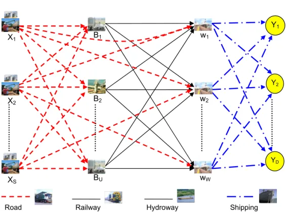
Spatial and temporal multimodal model flowchart
The objective of the spatial equilibrium model is to maximize the NSP function, thus maximizing the areas below the demand curves, plus the areas above the supply curves, minus the transportation and warehousing costs. The model uses the basic structure proposed by Takayama & Judge (1971), and Bivings (1997), whose origin lays in the pioneering work by Samuelson (1952). The main differences between the models discussed in the literature and the one proposed in this work are:
(a)The supply and demand functions are nonlinear; (b)Intermodal transportation;
(c)The transshipment points;
(d)The consideration of the temporal analysis as a proxy for warehousing; and (e)Warehousing costs.
Figure 2 – Network model of soybean transportation.
The supply and demand functions
As a consequence, considering the small production of the State of Tocantins – as will be examined later in the case study – some simplifications ought to be introduced in the supply and demand functions. Firstly, the state’s production is unable to have any measurable influence in international prices; therefore, the excess demand function might be seen as constant. Secondly, using eight years of available data, a simplified linear and nonlinear supply function of the following form was tested:
1 1
( , , , )
t t t
Hect = f Hect− Price− Year Dummy
where t
Hect = area in hectares planted in a given period t;
1
t
Price− = price of soybeans in period t-1;
Year = variable of tendency or time expressed in years;
Dummy= auxiliary variable.
Certainly, for a better adjustment the nonlinear equation would be recommended: 3
1 2 4
1 1
(0) (1) f (2) f (3) f (4) f
t t t
Hect =c +c Hect− +c Price− +c Year +c Dummy
YD Y2 Y1
X1
X2
XS
B1
B2
BU
w1
w2
wW
The exponents f1, f2, f3 and f4 are assumed to be rational numbers and the function takes the following form:
, in period
st st
a st st st
X =θ γ+ P ∀s t, which corresponds to (3.8)
4. The proposed model formulation
The indexes of the model are:
t: periods, (t = 1,2,...T);
d: consumer regions, (d = 1, 2,...D);
s: producer regions, (s = 1, 2,...S);
u: transshipment points, (u = 1,2,...U);
w: ports, (w = 1,2,...,W);
k: transportation mode (k = c, f, h), where c = trucks, f = railway, and h = hydroway. The variables involved are represented as:
NSP = Net Social Payoff Function; dt
λ = Cost-coefficient intercept of the demand equation d in period t; dt
ω = Cost-coefficient slope of the demand equation d in period t; st
ν = Cost-coefficient intercept of the supply equation s in period t; st
η = Cost-coefficient slope of the supply equation s in period t; dt
Y = Amount of soybeans consumed in region d in period t; st
X = Amount of soybeans supplied by region s in period t; c
sut
C = Unit transportation cost from region s to point u by trucks in period t; k
uwt
C = Unit transportation cost from point u to port w using mode k in period t; m
wdt
C = Unit transportation shipment from port w to overseas consumer d in period t; m
suwdt
X = Amount shipped from port w to overseas consumer d in period t; c
sut
X = Amount sent from region s to point u by trucks in period t; k
suwt
X = Amount sent from producer region s through point u to port w in period t using mode k;
m suwdt
X = Amount shipped overseas from points s, u and w to consumer d in period t;
, 1
AR st t
C + = Unit soybean warehousing cost in the producer region s in period t; AR
st
X = Amount of soybeans warehoused in region s in period t; TU
ut
C = Transshipment cost at point u in period t; TW
wt
C = Transshipment cost at port w in period t;
, 1
st t
The model includes the objective function (4.1), Max NSP, subjected to restrictions (4.2) through (4.7). All expressions are explained and justified further below.
(
)
(
)
1 1 1 1 1 1 1 1 1 1 NSP 1 1 1 1 1 1 dt dt dt dt st st st st bT D b
b
dt dt
b
dt dt dt dt
t d dt dt dt dt
a
T S a
a
st st
a
st st st st
t s st st st st
sut b b MAX Y b b a a X a a C
λ ω λ
ω ω
ν η ν
η η + + = = + + = = ⎡ ⎤ ⎢ ⎥ = ⋅ + − ⋅ ⋅ + + ⎢ ⎥ ⎣ ⎦ ⎡ ⎤ ⎢ ⎥ − ⋅ + − ⋅ ⋅ + + ⎢ ⎥ ⎣ ⎦ −
∑∑
∑∑
(
)
(
) (
)
(
)
(
)
1 1 1
T
t 1 1 1 1
1 1 1
* *
T U S
c c TU c
sut ut sut t u S
c c TW c f f TW f
W U S uwt suwt wt suwt uwt suwt wt suwt
h h TW h
w u s uwt suwt wt suwt
W U S
m m wdt suwdt d w u s
X C X
C X C X C X C X
C X C X
C X = = = = = = = = = = = + ⎡ + + + ⎤ ⎢ ⎥ − ⎢ ⎥ + + ⎣ ⎦ −
∑∑∑
∑ ∑∑∑
∑∑∑
(
)
1 1, 1 , 1
1 1 T D t T S AR AR st t st t t s C X = + + = = −
∑∑
∑∑
(4.1) subject to:(
)
(
)
dt1 1 1
, 1 1,
1
1
1
; , (4.2)
; , (4.3)
; , , (4.4)
; , , , (4.5)
W U S m suwdt w u s
U
c AR AR
sut st t st st t u
W
c f h c
suwt suwt suwt sut w
D
m c f h
suwdt suwt suwt suwt d
Y X d t
X X X X s t
X X X X s u t
X X X X s u w t
= = = + − = = = ≤ ∀ + ≤ + ∀ + + ≤ ∀ ≤ + + ∀
∑∑∑
∑
∑
∑
, 1 , 1
, 1
, (4.6)
, , , , , , , 0 (4.7)
AR
st t st t
c c f h m AR
dt st sut suwt suwt suwt suwdt st t
X CAP s t
Y X X X X X X X
+ +
+
≤ ∀
≥
The objective function, Max NSP, is to be understood as the excess demand, plus the excess supply, minus the costs of transportation, warehousing, and transshipment. The explanation is separated by parts:
(
)
1 1 1 1 1 1 1 1 dt dt dt dt bT D b
b
dt dt
b
dt dt dt dt
t d dt dt dt dt
b b
Y
b λ ω b λ
ω ω + + = = ⎡ ⎤ ⎢ ⋅ + + − ⋅ + ⋅ ⎥ ⎢ ⎥ ⎣ ⎦
∑∑
(
)
(
)
1
1 1 0
1 1 1 1 1 1 1 1 dt dt dt dt dt dt Y T D b dt dt dt dt t d
b
T D b
b
dt b dt
dt dt dt dt
t d dt dt dt dt
Y dY
b b
Y
b b
λ ω
λ ω λ
ω ω = = + + = = + ⎡ ⎤ ⎢ ⎥ = ⋅ + − ⋅ ⋅ + + ⎢ ⎥ ⎣ ⎦
∑∑ ∫
∑∑
Analogously, the integration of the supply function given in (3.3) from zero to Xst results in:
(
)
(
)
(
)
1
1 1 0
1 1 st 1 1 1 1 1
when 0;
1 1 1 whe 1 st st st st st st st st X
T S a
st st st st t s
a
T S a
a
st st
a
st st st st
t s st st st st
a st a st st st st X dX a a X a a a X a ν η
ν η ν ν
η η η η = = + + = = + + ⎡ ⎤ ⎢ ⎥
= ⋅ + − ⋅ ⋅ >
+ + ⎢ ⎥ ⎣ ⎦ ⎡ ⎤ = ⎢ ⋅ + ⎥ ⎣ ⎦
∑∑ ∫
∑∑
(
)
(
)
st 1 1 1 1 st 1 1 n 0; 1 1; 0;
1 1
st st
st st
T S
t s
T S a a
st st
a a
st st st st st st
t s st st st st
a a
X
a a
ν
ν η ν η θ ν
η η = = + + = = = ⎡ ⎤
= ⎢ ⋅ + + − ⋅ + ⋅ + ⎥ <
⎣ ⎦
∑∑
∑∑
The proposed model assumes that ν >st 0.
The transportation costs consider the four modes, and the total transportation costs from the producing regions to the transshipment points plus the transshipment costs are given by:
(
)
1 1 1
* *
T U S
c c TU c
sut sut ut sut t u S
C X C X
= = = +
∑∑∑
The total transportation costs from the transshipment points to the ports are given by the expression:
(
) (
)
(
)
T
t 1 1 1 1
c c TW c f f TW f
W U S uwt suwt wt suwt uwt suwt wt suwt
h h TW h
w u s uwt suwt wt suwt
C X C X C X C X
C X C X
= = = = ⎡ + + + ⎤ ⎢ ⎥ ⎢+ + ⎥ ⎣ ⎦
∑ ∑∑∑
The transportation costs from ports w to consumers d are given by:
(
)
1 1 1 1 1
T D W U S
m m wdt suwdt t d w u s
C X
= = = = =
∑∑∑∑∑
The warehousing costs are given by the expression:
(
, 1 , 1)
1 1
T S
AR AR st t st t t s
C + X +
= =
∑ ∑
(4.2) This restriction states that in each period the amount consumed in each region is smaller or equal to the amounts transported to the same region;
(4.3) This restriction states that in every period t for every producing region s
production plus the amount warehoused from period t-1 to t shall be larger or equal to the amount transported by trucks from this region to all transshipment points u in period t plus the stocks from t to t+1;
(4.4) Restrictions on the total quantities dispatched to all ports w, from each transshipment point u in each period t by all transport modes, which shall be smaller or equal to the quantities received at this transshipment point u by trucks from the given region s in the same period d;
(4.5) This restriction from ports to consumers states that for every port the volume sent to all consumers shall be smaller or equal to the amounts received from all producing regions for each period t;
(4.6) Warehousing capacity restriction for every producing region; (4.7) Non-negativity restrictions.
No capacity restriction was assigned to the transportation modes. Although capacities could be easily introduced in the model, the overlook of capacities seems realistic since the availability of trucks is elastic; the North-South Railway is projected to carry 15 million tons per year, a figure that largely surpasses the present production, and the hydroway designed capacity of two million tons per year is much larger than the present production or the one devised for the near future.
5. Results and discussion
In this section the results of the model are discussed and evaluated. Models that represent the real world may be quite useful if a careful validation of their effectiveness is previously done. The state of Tocantins is the object of a case study for which detailed data for the year 2005 has been collected including warehousing, spatial and temporal cost data. The results are then compared with the existing and projected infrastructure.
It is important to recall that the application was simplified to T = 2, which includes two yearly periods of unequal duration. One is the in-season that lasts three to four months, in which the harvest takes place. During this period, all tactical decisions such as selling, immediate exports, and warehousing have to be made. The second period is the rest of the year, or the out-of-season period, in which decisions are made regarding exports of the warehoused soybean.
The nonlinear spatial equilibrium model was applied for each one of the four devised scenarios, in order to find for each period: the exports, the best warehousing strategy, and the alternative routes by which the products may flow. Next, for each scenario, the results are summarized and the corresponding interpretations are assessed.
GAMS, General Algebraic Modeling System, was designed to solve linear, nonlinear, and integer programming models. Data are supplied either as text files, data sets or spread sheets and the models might be simply written. The results can be visualized and exported to text editors or spread sheets. The model developed for the case study was executed in a personal computer with 800 MHz Pentium III processor, 256 Mb RAM and Windows XP 2002 operational system. Execution time of the MINOS optimizer was around 0.031 seconds.
Scenario 1:
Scenario 1 corresponds to the present structure in which the soybeans are transported by trucks 385 km northwards until they reach the transshipment point in the Carajás Railway at the railway station of Estreito. The application of the model under these conditions results in the proposed solution portrayed in Figure 4. From the production point, the railway carries the product along 731 km until the port of Itaqui, 6,795 km away from Europe and 20,242 km from China.
Figure 4 – Production of soybeans in the state of Tocantins: exports, volume warehoused, and flow during and out of the harvesting period. (Scenario 1).
Scenario 2:
Scenario 2 corresponds to the proposed structure in which the Tocantins Hydroway is made operational. The application of the model under these conditions results in the solution portrayed in Figure 5. Accordingly, the soybeans make a short 20 km travel by trucks to reach the barges in the river, from where they journey 1,322 km to the port of Vila do Conde, 7,038 km away from Europe and 19,618 km from China.
Figure 5 – Production of soybeans in the state of Tocantins: exports, volume warehoused, and flow during and out of the harvesting period. (Scenario 2).
Scenario 3:
Scenario 3 corresponds to the proposed structure in which the soybeans are conveyed 20 km by trucks to the transshipment point at the Tocantins Hydroway, from where they travel 370 km northward to the railway station of Estreito. The application of the model under these conditions results in the proposed solution depicted in Figure 6. The railway carries the product along 731 km to the port of Itaqui, 6,795 km away from Europe and 20,242 km from China.
Figure 6 – Production of soybeans in the State of Tocantins: exports, volume warehoused, and flow during and out of the harvesting period. (Scenario 3).
Scenario 4:
Scenario 4 corresponds to the extension of the North-South Railway to the center of the state of Tocantins. The application of the model under these conditions results in the solution represented in Figure 7. Accordingly, the soybeans are transported 50 km by trucks to reach the transshipment point at the railway station of Guaraí, from where they journey 1,026 km up to the port of Itaqui and then to the European Union or China. The proposal is to export 60,598 tons during the in-season period and to warehouse 544,150 tons for exports in the out-of-season period. The total logistics cost per ton is US$ 39.06, while the Net Social Payoff objective function reaches US$ 233,103,900.
Figure 7 – Production of soybeans in the state of Tocantins: exports, volume warehoused, and flow during and out of the harvesting period. (Scenario 4).
6. The states of Maranhão and Piauí
Maranhão and Piauí are two neighboring states of Tocantins, as shown in Figure 1. Regarding their cultural background, historical development, and edaphic and climate factors these three states share many points in common. One is the presence of the cerrado biome in the southern part of Maranhão and Piauí, which drives the agricultural production towards similar products. Another common point is the early colonization based on an extensive cattle raising economy in which the herds used to move continuously in search of grass and the humans would follow them, eventually establishing small settlements in favorable areas. In contrast with most of the other states of the country, the geometrical form of the state of Piauí, being wide in the south and with a short ocean front, is often viewed as a confirmation of such occupation theory.
impact shipping costs from these inland areas to the international ports along the north and east coast. In addition, there is an absolute absence of warehousing facilities within every rural property, and the roadway network would be best described as an unpaved pathway network, hardly usable during the rain season.
In the case of Maranhão, the flow of products requires their transport to the production centroid of Balsas, from where 385 km of paved road convey the products to Imperatriz, where they are transshipped to the railway and move to the port of Itaqui. According to EMBRAPA (1997), apud Giordano (1999), in local currency freight costs per ton from the farms to Balsas averages R$ 17, from Balsas to Imperatriz R$ 12, from Imperatriz to Itaqui R$ 9.50, and from Itaqui to the port of Rotterdam R$ 27.70. According to the same study, these transportation costs represent US$ 68/ton, in contrast to similar farm-to-Rotterdam logistics costs of US$ 28 and US$ 43 in the United States and Argentina, respectively. In the state of Piauí the problems are similar, but access to the port of Itaqui, 611 km away from the production area, is made entirely by trucks through paved roads. Therefore, one single transportation mode over a not too distant port makes the operation more economical. In any case, production in this state is still smaller than in the other two, as shown by Table 1.
Table 1 – Recent soybean production in three states.
Year Production in tons
TO MA PI 2002 244,329 561,718 91,014 2003 377,638 660,078 308,225 2004 652,322 903,998 388,193 2005 905,328 996,909 559,545 2006 742,891 931,142 544,086
A complete study similar to that of Tocantins was not made for Maranhão and Piauí; only Scenario 1 was considered. Thus, for the existing transportation structure the results are summarized in Table 2.
Table 2 – Present total logistics costs for three states.
State Logistics cost per ton Tocantins (TO) US$ 40.10
Maranhão (MA) US$ 34.42
Piauí (PI) US$ 34.78
7. Conclusions
The global demand for soybeans is expanding very quickly since this is a valuable grain used in different forms by humans and by animals. The former use it as cooking oil and consume these beans as a rich and nutritious product, while the latter, around the world, have soybeans as one of the main ingredients for cattle raising and poultry production. In a number of poor countries, the present increase in domestic income is contributing to expand, usually indirectly, the demand for soybean. For example, a typical conversion rate of grain into meat is 2.8:1, i.e. an additional 1 million tons of meat would require 2.8 million tons of grain. Brazil appears to be the only country that has suitable land potentially able to be converted into large-scale soybean production and to export the additional production, since its cattle herd grazes and human consumption is limited. However, problems in the country’s infrastructure are restraining its faster development. Thus, the objective of this research was to propose a model for evaluating the competitiveness of soybean production in a recently occupied state in the northern part of the country, the state of Tocantins. In the area considered in the case study, productivity is very high, but the logistics to export the product is costly and very inefficient, although alternative routes might devised, evaluated, and developed. Since the product is exported in its raw form, the supply peak occurs during the harvest period, when transport tariffs are costly, all transport modes congested, and prices for the product depressed. Therefore, warehousing part of the production would reduce the incidence of these problems and help improve competitiveness.
In addition, the study has also examined the soybean production of the states of Maranhão and Piauí, that are neighbors of Tocantins and share similar difficulties. For these two states an evaluation of the existing logistics structure was carried out but no alternative scenarios have been developed. An interesting finding is that the production of Tocantins is less competitive than the one of the two states, but this situation might be reversed if the hydroway is made operational.
The present study has proposed a spatial multimodal and temporal equilibrium model expressed by a nonlinear programming model to evaluate a number of logistics routes for reaching the maritime ports at lower costs. The study has considered four different scenarios and this has reduced the size of the model. When the entire infrastructure depicted by these scenarios becomes available, a comprehensive model might be devised to determine mixed logistics strategies. Results of the study are interesting and suggest priorities in infrastructure investments to deal with a problem of national interest.
Acknowledgements
This first and second authors would like to thanks the CNPq, the National Council for Scientific and Technological Development of Brazil, who supported in part this research.
Note
References
(1) Bivings, E.L. (1997). The seasonal and spatial dimensions of sorghum market liberalization in México. American Journal of Agricultural Economics, 79, 383-393. (2) Bulhões, R. & Caixeta-Filho, J.V. (1999). Aplicação de um modelo de equilíbrio
espacial para análise da competição entre os portos de Paranaguá e Santos para movimentação de soja. In: Congreso Chileno de Ingeniería de Transportes 9, 1999. Santiago de Chile. Atas..., Santiago de Chile, 351-363.
(3) Caixeta Filho, J.V. & Macaulay, T.G. (1989). A utilização de modelos de equilíbrio espacial para a avaliação econômica de políticas agrícolas: estudo de caso australiano. In: XXVII Congresso Brasileiro de Economia e Sociologia Rural. São Paulo. Anais..., Sober, São Paulo, 232-245.
(4) Chen, C.-C.; McCarl, B.A. & Chang, C.-C. (2004). Spatial equilibrium modeling
with imperfectly competitive markets: an application to rice trade. Available at:
<http://agecon2.tamu.edu/people/faculty/mccarl-bruce/papers/736.pdf> Accessed on: 19 Jul. 2004.
(5) Cramer, G.L.; Wailes, E.J. & Shui, S. (1993). Impacts of liberalization trade in the world rice market. Agric. Econ., 75, 219-226.
(6) Dennis, S.M. (1999). Using spatial equilibrium model to analyze transportation rates: an application to steam coal in the Unites States. Transportation Research, part E, 35, 145-154.
(7) Fuller, S.; Fellin, L. & Salin, V. (2003). Effect of liberalized U.S.–México rice trade: A spatial, multiproduct equilibrium analysis. Agribusiness, 19, 1-17.
(8) Fuller, S.; Fellin, L.; Lalor, A. & Klindworth, K. (2000). Agricultural Transportation Challengers for the 21st Century: Effect of improving South American Transportation Systems on U.S. and South American Corn and Soybean Economies. Agricultural
Marketing Service, 1-40, Oct 2000.
(9) Gabriel, S.A.; Manik, J. & Vikas, S. (2001). Computational experience with a large-scale, multi-period, spatial equilibrium model of the North American natural gas system.
Network and Spatial Economics, 3, 97-122.
(10) Garcia, J.A. (1999). Distribución espacial e intertemporal de la producción de maíz en México. Montecillo, Texcoco. 158p. Teses (Doctoral en Ciencias). Colegio de Postgraduados en Ciencias Agrícolas.
(11) Garcia, J.A.; Matus, J.A.; Martinez, M.A.; Santiago, M. & Martinez, A. (2000). Determination of the optimal demand of maize storage in México. Agrociencia, 34, 773-784.
(12) GEIPOT – Empresa Brasileira de Planejamento de Transportes (1999). Corredores
Estratégicos de Desenvolvimento – Relatório Final. GEIPOT, Brasília.
(13) IBGE – Instituto Brasileiro de Geografia e Estatística (2007). Mapa Geográfico
Brasil-TO. Available at: <http://www.ibge.gov.br>. Accessed on: 3 Dec. 2007.
(15) Samuelson, P.A. (1952). Spatial Price Equilibrium and Linear Program. American
Economic Review, 42, 283-303.
(16) Takayama, T. (1995). Thirty years with spatial and intertemporal economics. The Annals
of Regional Science, 28, 305-322.
(17) Takayama, T. & Judge, G. (1964). Equilibrium among spatially separated markets: a reformulation. Econometrica, 519-524.
(18) Takayama, T. & Judge, G. (1971). Spatial and Temporal Price and Allocation Models. North Holland, Amsterdam. 528p.
(19) Tôsto, S.G. (1996). Mercado interno de grãos de soja: Modelos de equilíbrio e desequilíbrio. Viçosa, MG. 114p. Dissertação (Mestrado em Economia Rural). Universidade Federal de Viçosa.
(20) USDA–United States Department of Agriculture (2007). World agricultural outlook board.
<http://usda.mannlib.cornell.edu?mannUsda/viewDocumentInfo.do?documentID=1194>. Accessed on January 03, 2007.
(21) Waquil, P.D. (1996). Alocação ótima de produtos agropecuários no Mercosul: um modelo de equilíbrio espacial com produtos intermediários. Revista Brasileira de
Economia e Sociologia Rural, 34(1/2), 87-109, Brasília, Jan/Jun 1996.
(22) Yan, C.W. et al. (2002). The Cournot competition in the spatial equilibrium model.