ISSN 0104-6632 Printed in Brazil
www.abeq.org.br/bjche
Vol. 32, No. 04, pp. 903 - 917, October - December, 2015 dx.doi.org/10.1590/0104-6632.20150324s00003518
Brazilian Journal
of Chemical
Engineering
PREDICTION OF STABILITY AND THERMAL
CONDUCTIVITY OF SnO
2
NANOFLUID VIA
STATISTICAL METHOD AND AN ARTIFICIAL
NEURAL NETWORK
A. Kazemi-Beydokhti
1, H. Azizi Namaghi
2, M. A. Haj Asgarkhani
2and S. Zeinali Heris
3*1
Department of Chemical Engineering, School of Petroleum and Petrochemical Engineering, Hakim Sabzevari University, Sabzevar, Iran.
2Chemical Engineering Department, Faculty of Engineering, Ferdowsi University of Mashhad,
Mashhad, Iran.
3
Faculty of Chemical and Petroleum Engineering, University of Tabriz, Tabriz, Iran. E-mail: [email protected]; [email protected]; [email protected]
*E-mail: [email protected]
(Submitted: May 24, 2014 ; Revised: November 30, 2014 ; Accepted: January 9, 2015)
Abstract - Central composite rotatable design (CCRD) and artificial neural networks (ANN) have been applied to optimize the performance of nanofluid systems. In this regard, the performance was evaluated by measuring the stability and thermal conductivity ratio based on the critical independent variables such as temperature, particle volume fraction and the pH of the solution. A total of 20 experiments were accomplished for the construction of second-order polynomial equations for both target outputs. All the influential factors, their mutual effects and their quadratic terms were statistically validated by analysis of variance (ANOVA). According to the results, the predicted values were in reasonable agreement with the experimental data as more than 96% and 95% of the variation could be predicted by the respective models for zeta potential and thermal conductivity ratio. Also, ANN proved to be a very promising method in comparison with CCD for the purpose of process simulation due to the complexity involved in generalization of the nanofluid system.
Keywords: Nanofluid; Central composite design; Artificial neural network; Statistical; Stability; Thermal
conductivity.
INTRODUCTION
Nowadays, ultrahigh-performance of heating and cooling systems is one of the most vital needs of many industrial technologies, including power sta-tions, production processes, transportation, and elec-tronics. Many solutions such as heat surface addition (fins), vibration of the heated surface, injection or suction of fluid, applying electric or magnetic fields, and suspending nanoparticles with average sizes
Brazilian Journal of Chemical Engineering
Das et al., 2008; Kazemi-Beydokhti et al., 2013).
Long-term stability and thermal conductivity of nanofluids are important factors that have been widely investigated by many researchers for copper, aluminum, and titania nanoparticles with their oxides and carbon nanotubes (Murshed et al., 2005; Eastman, 2001; Hwang, 2006; Das et al., 2003a; Jiang and Wang, 2010; Lee et al., 1999; Salehi et al., 2011; Wang and Mujumdar, 2008(a,b); Molana and Ba-nooni, 2013).
Factors such as temperature, particle volume fraction, average primary particle size (APPS), pH of the nanofluid, elapsed time, ultrasonication (power and time), additive, base fluid and nanoparticle mate-rials affect the performance of nanofluid systems with different degrees of sensitivities. Kazemi-Beydokhti et al. (2013) applied a full foldover frac-tional factorial design (FFD) (
2
7 4III ) in order to
deter-mine which of the factors temperature, particle volume fraction, APPS, pH of the nanofluid, elapsed time, sonication time and density of the nanoparticles and their binary interactions have the greatest influ-ence on the results. The analysis of variance revealed that three factors, including the temperature, particle volume fraction and pH of the nanofluid, have the most significant effect on the response variable. Among the various types of nanoparticles, tin di-oxide, which has excellent chemical and physical stability, is not widely used, although it is a cheap and commercially available mineral product. In addi-tion, our previous work (Habibzadeh et al., 2010) on tin dioxide nanofluid confirms that these three fac-tors have a significant effect on stability and the ther-mal conductivity ratio.
The traditional methods of optimization such as one-factor-at-a-time (OFAT) experimental technique for multivariable systems can be used. However it is well accepted that this is time-consuming, excessive in cost, complicated and might provide the re-searcher with wrong conclusions. Also, factorial de-sign is weak in estimating quadratic terms and intro-ducing enough curvature into the response surface (Montgomery and Runger, 2003; Gheshlaghi, 2007; Gheshlaghi et al., 2008). To overcome such difficul-ties, a neural network and a multi-step statistical op-timization strategy involving factorial design and response surface methodology (RSM) have been de-veloped to analyze the effects of the process parame-ters on stability and the thermal conductivity of the nanofluid system. On the other hand, these tech-niques are good mathematical tools to build models, optimize the experimental results and obtain the opti-mal values of the output and input variables.
To the best of our knowledge, these techniques have not been applied for optimization of the main factor levels of stability and the thermal conductivity ratio of nanofluids. Therefore, the main objective of this study was to find the optimum conditions for maximizing the stability and thermal conductivity ratio of a tin dioxide nanofluid. In this regard, three independent variables, including temperature, parti-cle volume fraction and solution pH, were selected for modeling and optimization.
THEORETICAL
Response Surface Methodology (RSM)
Designing experiments is a statistically basic technique to obtain the most information in order to improve the performance of a manufacturing process from the fewest experimental runs. Among the vari-ous methods of designing experiments, response sur-face methodology is a combination of mathematical and statistical techniques that are useful for modeling and analyzing the influence of several design varia-bles on the response and the objective is to optimize this response (Montgomery and Runger, 2003; Gheshlaghi, 2007). The quadratic coefficients in the second-order model may be evaluated by applying 3 levels (at least) for each independent factor. As the number of independent factors increases in 3n facto-rial design, the number of required runs rapidly in-creases. Obviously, this may be unacceptable and lead to overkill if the experiments are time-consum-ing and costly. The central composite design (CCD) is a sequential design strategy which reduces the num-ber of experiments to get close to the 2-level full fac-torial design. Thus, 2n points of the full factorial two-level design may be combined with some center point repetition of nominal design and 2n axial runs to yield a CCD (Gheshlaghi, 2007; Gheshlaghi et al., 2008).
In this regard, in the present study, RSM based on the CCD has been applied for the modeling of the nanofluid system with the aid of Design Expert ver-sion 8.0.7.1 statistical software (Stat-Ease Inc.). Three independent design variables, namely tem-perature (X1), particle volume fraction (X2) and
solu-tion pH (X3), were investigated with the actual and
coded values shown in Table 1.
Table 1: Actual design variables with real and coded values for the CCD.
Independent variables
Symbol Coded and actual variable level Star-low Low Center High Star-high
-1.68 -1 0 1 1.68 Temperature
(C) X1 28 35 45 55 62
Particle volume fraction (%vol)
X2 1.3 2 3 4 4.7
Solution pH X3 4.6 6 8 10 11.4
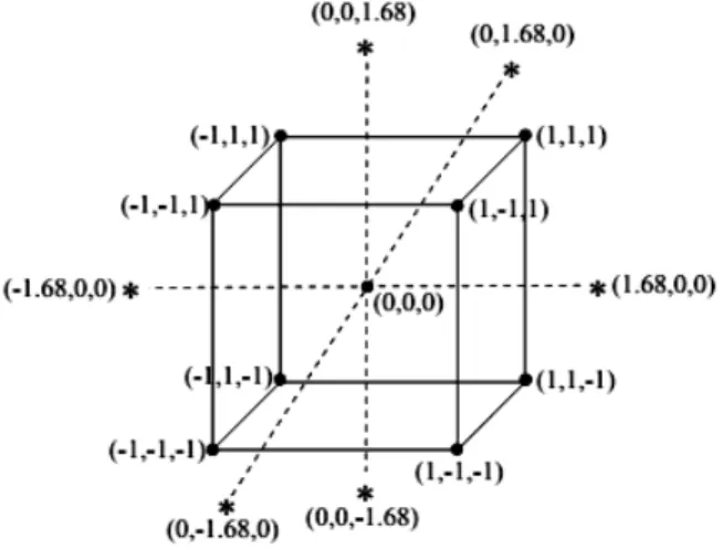
For the three factors, CCRD with a quadratic model is composed of the full 23 factors with its 8 cubic points, augmented with six replications of the center points and the six axial (star) points. Central composite designs with different properties can be developed by taking different values. To make the design rotatable, the axial distance was assigned a value of 1.68. Rotatable design makes the variance of prediction depend only on the scaled distance of the center of the design (Akhtar, 2001; Proust 2010). The CCD for the three independent factors is represented in Figure 1.
Figure 1: CCRD for the three significant factors.
To evaluate the efficiency of the statistical design of the experiment based on RSM, a multilayer feed-forward ANN was calculated.
Artificial Neural Networks (ANNs)
In recent years, the application of ANN has been developed as a powerful and flexible mathematical tool for modeling nonlinear and intricate systems. Also, an ANN can be considered as a massively
par-allel distributed processor, which transfers the knowledge and rules existing beyond the experi-mental data into the network structure for further applications (Rahmanian et al., 2011; Shanbedi et al., 2013; Salehi et al., 2013; Shanbedi et al., 2014). In this study, a multilayer feed-forward neural network has been used to design the complex non-linear relationships between input and output layers. Each layer has a specific number of neurons that play a significant role in the modeling of the system. The neurons in the input layer receive the data and then distribute them. The hidden layer processes and organizes the data received from the input layer and delivers them to the output layer (Yousefi et al., 2012). The output layer is the product of all the incoming signals. Finally the network was trained by using the Levenberg–Marquardt (LM) algorithm. The structure of this network is shown in Figure 2 schematically.
Figure 2: Schematic representation of the ANN for three input variables.
EXPERIMENTAL
Preparation of SnO2 Nanoparticles
Brazilian Journal of Chemical Engineering
Scherrer formula on the (1 1 0) diffraction peak. The BET surface area measurement was also carried out by nitrogen adsorption after degassing of the samples at 300 C for 2 hours, using a Quantachrome CHEMBET-3000 apparatus. All other information was mentioned in our previous work (Habibzadeh et al., 2010).
Sodium dodecyl sulfate, as an anionic surfactant, with the concentration of 0.1 mM, was selected and added in the preparation of nanofluids for better dis-persion of nanoparticles. Long term stability was not necessary for the measurement of thermal conduc-tivity of nanofluids by the Transient Hot Wire (THW) method because the measurements were made only a few seconds after preparation. Generally, the nano-fluids used in this study did not settle for at least 4 hours. Fluids with settling times less than three hours were excluded from the experiments.
Measurement of the Stability and Thermal Con-ductivity of the Nanofluid
Investigations show that clustering and aggrega-tion are main features in the stability and extraordi-nary enhancement of the thermal conductivity of nanofluids (Evans et al., 2008; Tucknott and Yaliraki, 2002). Hence, if we can prepare a more highly ho-mogenized nanofluid, the stability and thermal
con-ductivity of the nanofluid should be better. A stable suspension requires a good dispersion of the small particle in the liquid medium and a higher absolute value of the zeta potential of the particles (Tucknott and Yaliraki, 2002). Then, zeta potential was meas-ured by a Malvern Nano-ZS (Malvern Instrument Inc., London, UK). The pH was controlled by using hydrochloric acid (HCl) and sodium hydroxide (NaOH) of analytical grade. Thermal conductivity measurements were performed by a THW technique, which is known to be an accurate method for deter-mining the thermal conductivity of fluids. The details are elaborated elsewhere (Habibzadeh et al., 2010).
RESULTS AND DISCUSSION
Design of the Experiments and Response Surface Modeling
With respect to the previous sections, 20 different combination treatments were carried out in random order according to a CCD configuration and the re-sults of two responses, zeta potential (mV) and the thermal conductivity ratio were determined experi-mentally and predicted by the model according to the design. The results are summarized in Table 2.
Table 2: Design layout and experimental points of the CCRD.
Coded input variable Response variable
Std. Run A B C Zeta potential (mV) Thermal conductivity ratio Experimental Predicted Experimental Predicted
1 3 -1 -1 -1 Factorial design -19 -21.27 1.07 1.070
2 7 1 -1 -1 -27 -29.15 1.15 1.150
3 16 -1 1 -1 -25 -24.65 1.11 1.110
4 18 1 1 -1 -31 -32.53 1.19 1.190
5 9 -1 -1 1 -23 -25.43 1.09 1.094
6 14 1 -1 1 -34 -33.31 1.16 1.174
7 5 -1 1 1 -29 -28.81 1.13 1.134
8 15 1 1 1 -36 -36.69 1.23 1.214
9 11 -1.68 0 0 Axial points -27 -27.59 1.08 1.070
10 19 1.68 0 0 -40 -40.83 1.21 1.205
11 20 0 -1.68 0 -30 -27.98 1.17 1.146
12 10 0 1.68 0 -33 -33.66 1.22 1.214
13 17 0 0 -1.68 -21 -19.34 1.10 1.095
14 12 0 0 1.68 -26 -26.33 1.14 1.135
15 6 0 0 0 Center points -35 -34.21 1.18 1.180
16 8 0 0 0 -34 -34.21 1.16 1.180
17 2 0 0 0 -35 -34.21 1.20 1.180
18 1 0 0 0 -32 -34.21 1.17 1.180
19 4 0 0 0 -35 -34.21 1.19 1.180
A second-order polynomial equation was used to find the mathematical relationship between the de-pendent variables (zeta potential and thermal con-ductivity ratio) and the set of independent variables. For three factors, the obtained model was expressed as follows:
2 0
1 1
n i i n ii ii
n ij i ji i i j j
y b b x b x b x x (1)
where y represents the predicted responses, xi and xj
are the coded values of the independent variables, b0
is the regression term at the center point, bi are the
linear coefficients (main effect), bii are the quadratic
coefficients and bij are the two-factor interaction
co-efficients. Also, for statistical calculation based on CCD, the relation between the dimensionless coded values of the independent variables (xi) and the
ac-tual values of them (Xi) are defined as:
, ,
, ,
( ) / 2
( ) / 2
i i high i low i
i high i low
X X X
x
X X (2)
where Xi,high and Xi,low are the real values of the
inde-pendent variables at high and low levels, respectively.
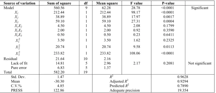
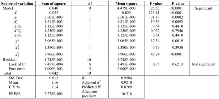
Analysis of Variance (ANOVA)
The ANOVA values for the quadratic regression model obtained from CCRD were employed in the
optimization of stability and thermal conductivity; which are respectively tabulated in Tables 3 and 4. With respect to these tables, the F-values of 28.78 and 25.63 implied that the models were statistically significant. There is only a 0.01% chance that model F-values this large could occur due to noise. Also, p-values less than 0.0500 indicate significant model terms. In the case of the responses in this study, the ranking of the significant model terms for zeta potential and the thermal conductivity ratio were
2 2
3 1 3 2 2
X X X X X and X1X32 X2 X12X3,
respectively. P-values, which are greater than 0.1, indicate insignificant model terms. The lack-of-fit F-values of 2.17 and 0.75 showed that the lack of fit of the models was not statistically important relative to the pure error. The insignificant lack of fit values are good and revealed that the quadratic models are statistically significant for the responses. Conse-quently, the following second order polynomial regression modeling was performed for the zeta potential (y1) and thermal conductivity ratio (y2) of
the nanofluid with coded variables:
1 1 2
2 2 3 2 3
34.21 3.94 1.69
2.08 1.2 4.03
y x x
x x x
(3)
2 1 2 3
2 2 1 3
1.18 0.04 0.02 0.012
0.015 0.023
y x x x
x x
(4)
Table 3: ANOVA for the quadratic regression model (response: zeta potential (mV)).
Source of variation Sum of square df Mean square F value P-value
Model 560.56 9 62.28 28.78 Significant <0.0001
X1 212.44 1 212.44 98.17 <0.0001
X2 38.89 1 38.89 17.97 0.0017
X3 59.10 1 59.10 27.31 0.0004
X1X2 4.50 1 4.50 2.08 0.1799
X1X3 2.00 1 2.00 0.92 0.3590
X2X3 0.50 1 0.50 0.23 0.6411
2 1
X 3.50 1 3.50 1.62 0.2325
2 2
X 20.74 1 20.74 9.58 0.0113
2 3
X 233.82 1 233.82 108.06 <0.0001
Residual 21.64 10 2.16
Lack of fit 14.81 5 2.96 2.17 0.2081 Not significant
Pure error 6.83 5 1.37
Total 582.20 19
Std. Dev.
1.47 R2 0.9628
Mean
-30.30 Adjusted R2 0.9294
C.V.%
4.85 Predicted R2 0.7890
PRESS
Brazilian Journal of Chemical Engineering
Table 4: ANOVA for the quadratic regression model (response: thermal conductivity ratio).
Source of variation Sum of square df Mean square F value P-value
Model 0.040 9 4.479E-003 25.63 Significant <0.0001
X1 0.022 1 0.022 126.11 <0.0001
X2 5.501E-003 1 5.501E-003 31.48 0.0002
X3 1.811E-003 1 1.811E-003 10.36 0.0092
X1X2 1.125E-004 1 1.125E-004 0.64 0.4410
X1X3 1.250E-005 1 1.250E-005 0.072 0.7946
X2X3 1.125E-004 1 1.125E-004 0.64 0.4410
2 1
X 3.065E-003 1 3.065E-003 17.54 0.0019
2 2
X 1.380E-004 1 1.380E-004 0.79 0.3950
2 3
X 7.906E-003 1 7.906E-003 45.24 <0.0001
Residual 1.748E-003 10 1.748E-004
Lack of fit 7.477E-004 5 1.495E-004 0.75 0.6213 Not significant
Pure error 1.000E-003 5 2.000E-004
Total 0.042 19
Std. Dev.
0.013 R2 0.9584
Mean
1.16 Adjusted R2 0.9210
C.V.%
1.14 Predicted R2 0.8269
PRESS
7.278E-003 Adequate
precision 16.518
The coefficient of determination (R2) expresses the quality of the fit of the polynomial model. The value of this statistical parameter for the zeta poten-tial (R2 = 0.9628) emphasizes that 96.28% of the variability in the response could be explained by the model and only 3.72% of the total variation was not explained by the model. The same interpretation applies to the other response variable. However, a concern with this statistic parameter is that it does not take the numbers of degree of freedom into ac-count for model determination. In other words, it always increases when new variables are added to the model, regardless of whether the additional vari-able is statistically significant or not. In order to negate this drawback, the adjusted coefficient of determination, R2-Adj, was used to adjust the varying numbers of degrees of freedom in the models. Tables 3 and 4 show that R2 and adjusted-R2 values for the models did not differ, obviously indicating that non-significant terms had not been included in the models.
The Predicted-R2 values of the stability and ther-mal conductivity ratio are 0.7890 and 0.8269, which are in reasonable agreement with the adjusted-R2 of 0.9294 and 0.9210, respectively. A rule of thumb is that the adjusted and predicted R-squared values should be within 0.2 of each other. Otherwise there may be a problem with either the data or the model. Adequate precision compares the range of pre-dicted values at the design points to the average
prediction error. A ratio greater than 4 is desirable to indicate adequate model discrimination. For our quadratic models, the ratios are 19.354 and 16.518 for the responses, indicating that the models give reasonable performance in predictions.
Statistical plots such as the normal probability plot and the studentized residuals versus different independent variables play significant roles in con-firming the normal error distribution, evaluating the final model adequacy and independently distributing the observations in a completely randomized design. In this regard, the normal percentage probability plots of the studentized residuals are shown in Figure 3. Regarding this figure, the residual points show that the error distribution was normal and no re-sponse transformation was required.
Internally Studentized Residuals
N
o
rm
a
l
%
P
ro
b
a
b
ili
ty
Normal Plot of Residuals
-3.00 -2.00 -1.00 0.00 1.00 2.00 1
5 10 20 30 50 70 80 90 95 99
Internally Studentized Residuals
N
o
rm
a
l
%
Pro
b
a
b
ili
ty
Normal Plot of Residuals
-2.00 -1.00 0.00 1.00 2.00 1
5 10 20 30 50 70 80 90 95 99
(a) (b)
Figure 3: Normal probability plot of residuals for zeta potential (a) and the thermal conductivity ratio (b) of the tin dioxide nanofluid system.
3 2
Predicted
In
te
rn
a
lly
S
tu
d
e
n
ti
z
e
d
R
e
si
d
u
a
ls
Residuals vs. Predicted
-3.00 -2.00 -1.00 0.00 1.00 2.00 3.00
-40.00 -35.00 -30.00 -25.00 -20.00 -15.00
2
Predicted
In
te
rn
a
lly
S
tu
d
e
n
ti
z
e
d
R
e
s
id
u
a
ls
Residuals vs. Predicted
-3.00 -2.00 -1.00 0.00 1.00 2.00 3.00
1.05 1.10 1.15 1.20 1.25
(a) (b)
Figure 4: Plot of studentized residuals versus predicted responses for the zeta potential (a) and thermal conductivity ratio (b) in the tin dioxide nanofluid system.
Effect of Selected Factors on the Zeta Potential of the Nanofluid
The major challenge in nanofluid systems is the rapid settling of the nanoparticles in fluids. The zeta potential decline is caused by several factors such as nanoparticle clustering, agglomeration and close packing of the dispersed phase. Thus, in order to ob-tain a better understanding of the results, the
Brazilian Journal of Chemical Engineering
It was observed that the zeta potential decreases (stability increased) upon increasing temperature and particle volume fraction. These facts should take into account that the temperature directly regulates parti-cle kinetic energies, Brownian motion of nanoparti-cles and finally the coagulation efficiency. Therefore, if the kinetic energy of the particles is lower than their interaction potential, coagulation of two parti-cles occurs after collision. Also, the formation proba-bility of bigger agglomerates increases at low tem-peratures (Fiedler et al., 2007; Ghosh et al., 2011; Chang et al., 2005). This can also be explained by the significant positive quadratic term (x22) and negative linear term (x2) in Eq. (3). According to this equation, the zeta potential (y1) decreased based on a negative linear term and increased based on a positive quad-ratic term.
It is clear from Figure 5 that the stability in-creases upon increasing SnO2 concentration. This behavior could be explained by two effects. First of all, the viscosity of a nanofluid is higher than that of its base fluid and increases with an increase in the particle volume concentration (Goharshadi et al., 2013). Secondly, due to the high surface area and surface activity, nanoparticles have the tendency to aggregate. The use of efficient surfactant is another key method to enhance the stability of nanoparticles in the base fluid (Yu et al., 2012). Surfactants play a very crucial role in nanofluid systems. The concen-tration of the surfactant has a positive effect on the dynamic viscosity of nanofluids and prevents the nanoparticle agglomeration due to the increase of
electrostatic repulsion between the suspended parti-cles. Consequently, adding surfactant significantly minimizes particle aggregation and enhances the dis-persion behavior (Goharshadi et al., 2013; Hwang et al., 2007; Hwang et al., 2008). Although the increase in nanoparticle concentration improves stability, the agglomeration is more obvious at concentrations over 5% (Pirahmadian and Ebrahimi, 2012). This can also be explained by the significant quadratic term x22 in Eq. (3).
Figure 6 shows the effect of solution pH versus temperature at a constant nanoparticle concentration of 3% by volume. The maximum response zone of stability is observed at pH values of 7 to 8.25 at each temperature level. This illustrates that increasing the pH up to 7-8 will enhance stability. This behavior is due to the fact that the stability of a nanofluid is re-lated to its electrokinetic properties. At the isoelectric point (IEP), the repulsive forces between SnO2 nano-particles tend towards zero and nanonano-particles will coagulate together at this pH value.
The hydration forces between nanoparticles increase as the pH of the solution departs from the IEP, which results in the enhanced mobility of nanoparticles in the suspension and the colloidal particles become more stable (Habibzadeh et al., 2010; Goharshadi et al., 2013). At high and low levels of solution pH, stability has a tendency to decrease. Theoretically, this may be attributed to the decrease of the surface charge. As a result, a weakly repulsive double layer force is generated
-1.00 -0.50 0.00 0.50 1.00 -1.00
-0.50 0.00 0.50
1.00 Zeta potential
A: Temperature
B:
Pa
rt
ic
le
v
o
lu
m
e
f
ra
c
ti
o
n
-36 -34
-32
-30
-28
6
-1.00 -0.50
0.00 0.50
1.00
-1.00 -0.50 0.00 0.50 1.00 -40
-35 -30 -25 -20
Z
e
ta
p
o
te
n
ti
a
l
A: Temperature B: Particle volume fraction
(a) (b)
-1.00 -0.50 0.00 0.50 1.00 -1.00
-0.50 0.00 0.50
1.00 Zeta potential
A: Temperature
C
:
So
lu
ti
o
n
p
H
-35
-30
-25
6
-1.00 -0.50
0.00 0.50
1.00
-1.00 -0.50 0.00 0.50 1.00 -40
-35 -30 -25 -20
Z
e
ta
p
o
te
n
ti
a
l
A: Temperature C: Solution pH
(a) (b)
Figure 6: Response surface and contour plots showing the mutual effect of temperature and pH on zeta potential while the other factor was kept constant at the center point (X2=3% by volume).
The interaction effect of particle volume fraction and solution pH at a constant temperature of 45 C on zeta potential is depicted in Figure 7. As shown in this figure, there is an enough curvature in this plot and the response surface is moderately nonlinear. In order to capture the curvature of the response in the
design space, significant quadratic terms such as x22
and x32 were taken into account in Eq. (3). The same interpretation is applied for pH and the concentration of nanoparticles on the stability of the nanofluid. The contour plot shows that the process is more sensitive to a change in pH than in particle volume fraction. The optimum is close to the pH of 8 and a particle volume fraction of 3.5% by volume.
-1.00 -0.50 0.00 0.50 1.00 -1.00
-0.50 0.00 0.50
1.00 Zeta potential
B: Particle volume fraction
C
:
So
lu
ti
o
n
p
H -34
-32
-30 -28
-26
6
-1.00 -0.50
0.00 0.50
1.00
-1.00 -0.50 0.00 0.50 1.00 -40
-35 -30 -25 -20
Z
e
ta
p
o
te
n
ti
a
l
B: Particle volume fraction C: Solution pH
(a) (b)
Brazilian Journal of Chemical Engineering Effect of Selected Factors on the Thermal
Con-ductivity Ratio
Previous experimental studies showed that the thermal conductivity enhancement of nanofluids de-pends on several mechanisms such as Brownian mo-tion of the nanoparticles, clustering of the nanoparti-cles and liquid layering around the nanopartinanoparti-cles (Pi-rahmadian and Ebrahimi, 2012; Ghadimi et al., 2011). These phenomena can also be described by several significant factors such as temperature, parti-cle volume fraction, pH of the nanofluid, etc. In this regard, the 3D response surface plots and contour line map of the predicted models for the thermal con-ductivity ratio of nanofluid are presented in Figures 8-10.
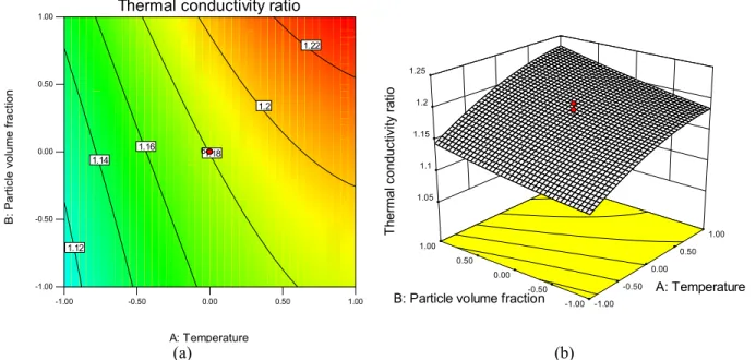
Figure 8 demonstrates the variations in the ther-mal conductivity ratio in terms of the temperature and particle volume fraction variables while the solu-tion pH was kept constant at the center point. By con-sidering this figure, increasing the temperature from 35 to 55 C increases the thermal conductivity to 7.47% and 6.44% at the high level and the low level of the particle volume fraction, respectively. These enhancements in thermal conductivity can be ade-quately explained by kinetic theory; Brownian move-ment (stochastic motion of molecules and nanoparti-cles) increases with the increase of the nanofluid's bulk temperature. Consequently, these particles are able to transfer more energy from one place to an-other per time unit. On the an-other hand, these en-hancements are due to a reduction in the clustering
effect which is intensified by an increase in tempera-ture (Das et al., 2003b).
Most experimental observations of nanofluid sys-tems show that the thermal conductivity ratio in-creases remarkably with the increase of particle vol-ume fraction. This behavior is also evident in Figures 8 and 10. This phenomenon is attributed to the fact that the collision of nanoparticles with each other is increased by increasing the nanoparticle concentra-tion. Although the probability of nanoparticle agglom-eration increases with increasing particle volume fraction, dispersing agents such as SDS reduce the van der Waals forces and improve nanoparticle dispersion. It was also observed that the rate of change of the thermal conductivity with temperature and particle volume fraction was dependent on the pH value, as shown in Figures 9 and 10, respectively. This is due to the fact that the pH value strongly influences the electrostatic charge of the particle surface. The ther-mal conductivity ratio increases with pH, reaches a maximum close to the isoelectric point and decreases as the pH increases further.
At the optimum value of the pH (approximately between 8 and 9) for maximum thermal conductivity enhancement, the surface charge of nanoparticles increases, which creates a high electrostatic repul-sion between nanoparticles. Consequently, the mo-bility of tin dioxide nanoparticles is enhanced and severe clustering and agglomeration of the nanoparti-cles are prevented (Shanbedi et al., 2014; Goharshadi
et al., 2013; Ranakoti Irtisha et al., 2012; Xian-Ju and
Xin-Fang, 2009).
-1.00 -0.50 0.00 0.50 1.00 -1.00
-0.50 0.00 0.50
1.00 Thermal conductivity ratio
A: Temperature
B
:
Pa
rt
icl
e
vo
lu
me
f
ra
ct
io
n
1.12 1.14
1.16
1.18 1.2
1.22
6
alue
-1.00 -0.50 0.00 0.50 1.00
-1.00 -0.50
0.00 0.50
1.00 1.05
1.1 1.15 1.2 1.25
T
h
e
rma
l
c
o
n
d
u
c
ti
v
it
y
ra
ti
o
A: Temperature B: Particle volume fraction
(a) (b)
-1.00 -0.50 0.00 0.50 1.00 -1.00
-0.50 0.00 0.50
1.00 Thermal conductivity ratio
A: Temperature
C
:
So
lu
ti
o
n
p
H
1.1 1.12
1.14
1.16 1.18
1.2
6
alue
-1.00 -0.50 0.00 0.50 1.00
-1.00 -0.50
0.00 0.50
1.00 1.05
1.1 1.15 1.2 1.25
T
h
e
rma
l
c
o
n
d
u
c
ti
v
it
y
ra
ti
o
A: Temperature C: Solution pH
(a) (b)
Figure 9: Response surface and contour plots showing the mutual effect of temperature and pH on the thermal conductivity ratio while the third factor was kept constant at the center point (X2=3% volume).
-1.00 -0.50 0.00 0.50 1.00 -1.00
-0.50 0.00 0.50
1.00 Thermal conductivity ratio
B: Particle volume fraction
C
:
So
lu
ti
o
n
p
H
1.14
1.16 1.16
1.18
1.2
6
e
-1.00 -0.50 0.00 0.50 1.00
-1.00 -0.50
0.00 0.50
1.00 1.05
1.1 1.15 1.2 1.25
T
h
e
rm
a
l
c
o
n
d
u
c
ti
v
it
y
ra
ti
o
B: Particle volume fraction C: Solution pH
(a) (b)
Figure 10: Response surface and contour plots showing the mutual effect of particle volume fraction and pH on the thermal conductivity ratio while the third factor was kept constant at the center point (X1=45 C).
Optimization of the Operational Conditions
The final optimum experimental results based on RSM strategy were calculated by the software to de-termine the optimum settings for the factors. The optimal experimental conditions based on the coded factors and the responses were carried out by mini-mizing the zeta potential and maximini-mizing thermal conductivity ratio and are reported in Table 5. With respect to this table, all three factors were limited to
their lower and upper coded values. The default is for both responses to be equally important in a set-ting of 3 pluses (+++). The optimal process condi-tions determined by the CCRD method based on the actual values of the factors are as follows: X1 = 55 C,
X2 = 3.36% by volume and X3 = 8.62; in these
condi-tions, a zeta potential of -38.22 mV was obtained in result 1. The value of 1.23 was obtained for the maximum thermal conductivity ratio at X1 = 54.4 C,
Brazilian Journal of Chemical Engineering
Under the optimal experimental conditions for both responses, a zeta potential of -37.98 mV and thermal conductivity ratio of 1.23 were determined at
X1 = 55 C, X2 = 3.81% by volume and X3 = 8.6 in
result 3.
Table 5: Optimum values of the design criteria for the zeta potential and thermal conductivity ratio for the tin dioxide nanofluid.
Optimum result
Coded factors Zeta potential
(mV)
Thermal conductivity
ratio
Desirability
x1 x2 x3
1 1 0.36 0.31 -38.22 ---- 0.915
2 0.94 0.98 0.42 ---- 1.23 1
3 1 0.81 0.3 -37.98 1.23 0.951
Artificial Neural Networks Modeling
Figure 11 shows the regression plots for the output with respect to training, validation, and test data. With respect to this figure, the output tracks the targets quite well and the R-value is over 0.995. Consequently, neural networks are able to predict the present nanofluid system.
The ability of the ANN model and its accuracy for this system are shown by the comparison between the values predicted by the ANN model and experimental data that were not used in training of the ANN, as presented in Figure 12. The proximity of the points to the diagonal line in Figure 12 indicates that the ANN provides results very close to the experimental measurements and confirms the accuracy of the ANN model.
Figure 11: Network model with training, validation, test and the full prediction set.
To show the accuracy of the model, the absolute average relative error (AARE) and standard deviation (Std. Dev.) for N data were calculated as follow (Gheshlaghi, 2007):
1
% 100
N experimental calculation
i i
experimental i
i
X X
X AARE
N (5)
2
1
1
% . . 100
1
N experimental calculation
i i
experimental i
i
X X
Std Dev AARE
N X (6)
Table 6 lists the %AARE and %Std. Dev. values for the zeta potential and thermal conductivity ratio. Because the AARE values for both parameters are very small and close to zero, we can conclude that the ANN model is suitable for the prediction of this nanofluid system and that the prediction values are reliable (Rahmanian et al., 2011).
Table 6: AARE and Std. Dev. for zeta potential and thermal conductivity ratio which modeled by ANN.
Parameter Method %AARE %Std. Dev.
Zeta potential ANN 0.872 1.121
Thermal conductivity ratio
ANN 0.376 0.268
CONCLUSION
The performance of the nanofluid system was modeled and expressed in terms of the stability and thermal conductivity content of the nanoparticles. In this regard, the effect of varying temperature, parti-cle volume fraction and the pH of solution were in-vestigated using RSM and ANN methods. The re-sults clearly show that CCRD and the ANN model can be used for the modeling of the SnO2 nanofluid system. ANOVA analysis indicated that there is sig-nificant curvature in the design space. Consequently, the quadratic models were statistically fitted to cap-ture the curvacap-ture using CCRD. A multilayer neural network was also used, which is effective for finding complex non-linear relationships. This mathematical model was found to be a reliable predictive tool with an excellent accuracy, with AARE of ±0.872% and ±0.376% in comparison with experimental values for the zeta potential and thermal conductivity ratio, re-spectively. Finally, the optimization demonstrated that a temperature of 55 C, particle volume fraction
of 3.81% volume and pH=8.6, provided the maximum stability and thermal conductivity enhancement.
ACKNOWLEDGEMENTS
The authors would like to thank the Iran Nano Technology Initiative Council for financial support of this project.
NOMENCLATURE
n Number of main factor
Xi Actual value of independent design variable
A or X1 Temperature (°C)
B or X2 Particle volume fraction (% volume)
C or X3 Solution pH
b0 Regression term at the center point
bi The linear coefficients (main effect)
bii The quadratic coefficients
bij The two-factor interaction coefficients
xi and xj
The coded values of independent design variables
Xi,high
Real value of the independent variable at the high level
Xi,low
Real value of the independent variable at the low level
y Predicted response with coded variables
y1
Zeta potential of nanofluid with coded variables (mV)
y2
Thermal conductivity ratio of nanofluid with coded variables
R2 Coefficient of determination
R2-Adj Adjusted coefficient of determination
df Degree of freedom
C.V. Coefficient of variation
Std. Dev.Standard deviation
Brazilian Journal of Chemical Engineering
Greek Symbols
α Distance of each axial point (also called star point) from the center
REFERENCES
Akhtar, M., Five-factor central composite designs robust to a pair of missing observations. J. Res. Sci., 12(2), 105-115 (2001).
Chang, H., Lo, C. H., Tsung, T. T., Cho, Y. Y., Tien, D. C., Chen, L. C., Thai, C. H., Temperature ef-fect on the stability of CuO nanofluids based on measured particle distribution. Key Eng. Mater., 295-296, 51-56 (2005).
Das, S. K., Choi, S. U. S., Yu, W., Pradeep, T., Nanofluids: Science and Technology. John Wiley & Sons, Hoboken, New Jersey (2008).
Das, S. K., Putra, N., Thiesen, P., Roetzel, W., Tem-perature dependence of thermal conductivity en-hancement for nanofluids. J. Heat Transfer, 125, 567-574 (2003a).
Das, S. K., Putta, N., Thiesen, P., Roetzel, W., Tem-perature dependence of thermal conductivity en-hancement for nanofluid. ASME Trans. J. Heat Transf., 125, 567-574 (2003b).
Eastman, J. A., Choi, S. U. S., Li, S., Yu, W., Thomp-son, L. J., Anomalously increased effective thermal conductivities of ethylene glycolbased nanofluids containing copper nanoparticles. Appl. Phys. Lett., 78, 718-720 (2001).
Evans, W., Prasher, R., Fish, J., Meakin, P., Phelan, P., Keblinski, P., Effect of aggregation and inter-facial thermal resistance on thermal conductivity of nanocomposites and colloidal nanofluids. Int. J. Heat Mass Transfer, 51, 1431-1438 (2008). Fiedler, S. L., Izvekov, S., Violi, A., The effect of
tem-perature on nanoparticle clustering. Carbon, 45, 1786-1794 (2007).
Ghadimi, A., Saidur, R., Metselaar, H. S. C., A Re-view of nanofluid stability properties and charac-terization in stationary conditions. Int. J. Heat Mass Transfer, 54, 4051-4068 (2011).
Gheshlaghi, R., Optimization of Recombinant Pro-tein Production by a Fungal Host. Ph.D. Thesis, Waterloo, Ontario, Canada (2007).
Gheshlaghi, R., Scharer, J. M., Moo-Young, M., Douglas, P. L., Application of statistical design for the optimization of amino acid separation by reverse-phase HPLC. Anal. Biochem., 383, 93-102 (2008).
Ghosh, M. M., Roy, S., Pabi, S. K., Ghosh, S., A Mo-lecular dynamics-stochastic model for thermal
conductivity of nanofluids and its experimental validation. J. Nanosci. Nanotechnol., 10, 196-207 (2011).
Goharshadi, E. K., Ahmadzadeh, H., Samiee, S., Hadadian, M., Nanofluids for Heat transfer en-hancement-a review. Phys. Chem. Res., 1(1), 1-33 (2013).
Habibzadeh, S., Kazemi-Beydokhti, A., Khodadadi, A. A., Mortazavi, Y., Omanovic, S., Shariat-Niassar, M., Stability and thermal conductivity of nanofluids of tin dioxide synthesized via micro-wave-induced combustion route. Chem. Eng., J., 156, 471-478 (2010).
Hwang, Y. J., Ahn, Y. C., Shin, H. S., Lee, C. G., Kim, G. T., Park, H. S., Lee, J. K., Investigation on characteristics of thermal conductivity en-hancement of nanofluids. Curr. Appl. Phys., 6, 1068-1071 (2006).
Hwang, Y., Lee, J. K., Jeong, Y. M., Cheong, S. I., Ahn, Y. C., Kim, S. H., Production and dispersion stability of nanoparticles in nanofluids. Powder Technol., 186, 145-153 (2008).
Hwang, Y., Lee, J. K., Lee, C. H., Jung, Y. M., Cheong, S. I., Lee, C. G., Ku, B. C., Jang, S. P., Stability and thermal conductivity characteristics of nanofluids. Thermochimica Acta, 455, 70-74 (2007).
Jiang, W., Wang, L. Q., Copper nanofluids: Synthesis and thermal conductivity. Curr. Nanosci., 6, 512-519 (2010).
Kazemi-Beydokhti, A., Azizi-Namaghi, H., Zeinali Heris, S., Identification of the key variables on thermal conductivity of CuO nanofluid by a frac-tional factorial design approach. Numer. Heat Transfer-Part B, Fundamentals, 64, 480-495 (2013). Lee, S., Choi, S. U. S., Li, S., Eastman, J. A., Meas-uring thermal conductivity of fluids containing oxide nanoparticles. J. Heat Transf., 121, 280-289 (1999).
Molana, M. and Banooni, S., Investigation of heat transfer processes involved liquid impingement jets: A review. Braz. J. Chem. Eng., 30 (3), 413-435 (2013).
Montgomery, D. C., Runger, G. C., Applied Statistics and Probability for Engineers. 3rd Ed., John Wiley & Sons, New York, U.S.A (2003).
Proust, M., Design of Experiments Guide. SAS Insti-tute Inc., Cary, NC, USA (2010).
Rahmanian, B., Pakizeh, M., Mansoori, S. A. A., Abedini, R., Application of Experimental design approach and Artificial Neural Network (ANN) for the determination of potential micellar-en-hanced ultrafiltration process. J. Hazard Mater. 187, 67-74 (2011).
Ranakoti Irtisha, G., Dewangan, S., Kosti, S., Nemade, R., Heat Transfer Enhancement by Nano Fluids. Convective Heat Mass Transfer, ME642, 1-9 (2012).
Salehi, H., S. Zeinali Heris, H., Koolivand Salooki, M., Noei, S. H., Designing a neural network for closed thermosyphon with nanofluid using ge-netic algorithm. Braz. J. Chem. Eng., 28(1), 157-168 (2011).
Salehi, H., Zeinali Heris, S., Esfandyari, M., Kooli-vand, M., Nero-fuzzy modeling of the convection heat transfer coefficient for the nanofluid. Heat Mass Transfer, 49, 575-583 (2013).
Shanbedi, M., Jafari, D., Amiri, A., Zeinali Heris, S., Baniadam, M., Prediction of temperature perfor-mance of a two-phase closed thermosyphon using artificial neural network. Heat Mass Transfer, 49, 65-73 (2013).
Shanbedi, M., Zeinali Heris, S., Amiri, A., Adyani, S., Alizadeh, M., Baniadam, M., Optimization of
ther-mal efficiency of a two-phase closed thermosy-phon using active learning on the human algo-rithm interaction. Numer. Heat Transfer-Part A: Applications, 66(8), 947-962, (2014).
Tucknott, R., Yaliraki, S. N., Aggregation properties of carbon nanotubes at interfaces. Chem. Phys., 281, 455-463 (2002).
Wang, X. Q., Mujumdar A. S., A review on nanoflu-ids - part II: Experiments and applications. Braz. J. Chem. Eng., 25(4), 631-648 (2008a).
Wang, X. Q., Mujumdar, A. S., A review on nano-fluids – part I: Theoretical and numerical inves-tigations. Braz. J. Chem. Eng., 25(4), 613-630 (2008b).
Xian-Ju, W., Xin-Fang, L., Influence of pH on nanofluids’ viscosity and thermal conductivity. Chin. Phys. Lett., 26(5), 1-4 (2009).
Yousefi, F., Karimi, H., Papari, M. M., Modeling viscosity of nanofluids using diffusional neural networks. J. Mol. Liq., 175, 85-90 (2012).
Yu, W., Xie, H., A review on nanofluids: Preparation, stability mechanisms and application. J. Nano-mater., 2012(1), 1-17 (2012).