ISSN 0104-6632 Printed in Brazil
www.abeq.org.br/bjche
Vol. 32, No. 02, pp. 563 - 575, April - June, 2015 dx.doi.org/10.1590/0104-6632.20150322s00003160
Brazilian Journal
of Chemical
Engineering
MODELLING OF DISPLACEMENT WASHING
OF PULP FIBERS USING THE HERMITE
COLLOCATION METHOD
S. Arora
1, I. Kaur
1and F. Pot
ůč
ek
2* 1Department of Mathematics, Punjabi University, Patiala-147002, India.E-mail: [email protected]; [email protected] 2
Department of Wood Pulp and Paper, University of Pardubice, Pardubice, Czech Republic. *E-mail: [email protected]
(Submitted: December 9, 2013 ; Revised: July 22, 2014 ; Accepted: August 24, 2014)
Abstract - A non-linear mathematical model for displacement washing of pulp fibers with suitable boundary
conditions is presented. Model equations are divided into two phases: particle phase and external fluid phase. The Hermite collocation method (HCM) is employed to solve the non-linear model equations. The validity and efficiency of the proposed model is demonstrated by comparing the numerical results with the experimental ones. Stability of the proposed method is checked by evaluating L2 and L∞ norms at different
time intervals. Industrial parameters such as displacement ratio and wash yield have been calculated to check the validity of the model. Numerical values obtained from the model equations are presented in terms of 2D graphs.
Keywords: Cubic Hermite polynomials; Peclet number; Biot number; Wash yield; Displacement ratio; Bed porosity.
INTRODUCTION
Applications of mathematical techniques for the solution of mass transfer problems in the field of chemical and process industries has always been the centre of study for mathematicians, as well as for chemical engineers. The diffusion dispersion problems arising from packed bed reactors have always moti-vated the scientists for the development of new models (Pellet, 1966; Grähs, 1974; Neretnieks, 1974, 1976; Perron & Lebeau, 1977; Al-Jabari et al., 1994; Kukreja
et al., 1995; Eriksson et al., 1996; Potůček, 1997;
Potůček & Pulcer, 2004; Arora et al., 2006, 2008). It has given rise to the use of a variety of analytical and numerical techniques for the solution of these models such as Laplace transforms (Brenner, 1962; Pellett, 1966; Rasmuson & Neretnieks, 1980; Liao & Shiau, 2000; Aminikhah, 2012), orthogonal collocation method (Villadsen & Stewart, 1967; Michelsen &
Villadsen, 1971; Raghvan & Ruthven, 1983; Ado-maitis & Lin, 2000; Solsvik & Jakobsen, 2012), or-thogonal collocation on finite elements (Carey & Finlayson, 1975; Ma & Guiochon, 1991; Arora et al.,
2005, 2006, 2008), Galerkin method (Liu & Bhatia, 2001; Onah, 2002; Bhrawy & El-Soubhy, 2010; Nadukandi et al., 2010; Shen et al., 2011; Zhu et al.,
Brazilian Journal of Chemical Engineering compared to particles having cylindrical geometry,
e.g., fibers. Due to the highly porous nature and com-plex particle geometry of pulp fibers and rigidity in the computational approach, the majority of investi-gators have preferred the study of glass beads and granular particles instead of pulp fibers. The rate of removal of the soluble impurities from the pores of the particles is slower than that from the interstices of the particles, due to the relatively small pore size. Therefore, diffusion through the pores of particles is expected to control the overall washing rate (Pellett, 1966; Han, 1967).
The objective of the present study was to develop a mathematical model for the analysis of washing of the porous structure of particles, especially fibers. The prime motive of washing is to remove the solu-ble impurities adsorbed on the particle surface using external aid. For porous particles the solute must diffuse out before it is dispersed by the flowing liquid. The solute from the irregular void channels of the bed is displaced and coupled with diffusion-like dis-persion of washing liquid in the direction of flow. Due to the adsorption of solute on the fiber surface, mass transfer occurs through the particle pores to particle surface and from particle surface to external fluid.
Dilution/extraction and displacement washing are basically two types of pulp-washing operations. In the former case the pulp slurry is diluted and thor-oughly mixed with wash liquor and then filtered for thickening. In the latter case the liquor in the pulp bed is displaced with wash liquor. However, if the same amount of wash liquor is used, displacement washing is better than dilution/extraction (Potůček, 1997).
MODEL DEVELOPMENT
Fluid concentration in packed beds of porous par-ticles is mainly based on two types of mechanisms. One is related to the transfer rate between fluid and particles and is given explicitly by the differential
equation q f n q( , )
t
Δ
∂ =
∂ .
This type of mechanism has been discussed widely for both linear and non-linear isotherms (Brenner, 1962; Sherman, 1964; Grähs, 1974; Potůček, 1997; Potůček & Pulcer, 2004; Arora & Potůček, 2012). In the second type of rate mechanism, the function
( , )
f n q is replaced by an integral equation signifying
the solid phase diffusion into the interior of the parti-cles. In this paper, second type of rate mechanism
has been followed for a Langmuir adsorption iso-therm to study the displacement washing of fluid flow through the packed bed of particles.
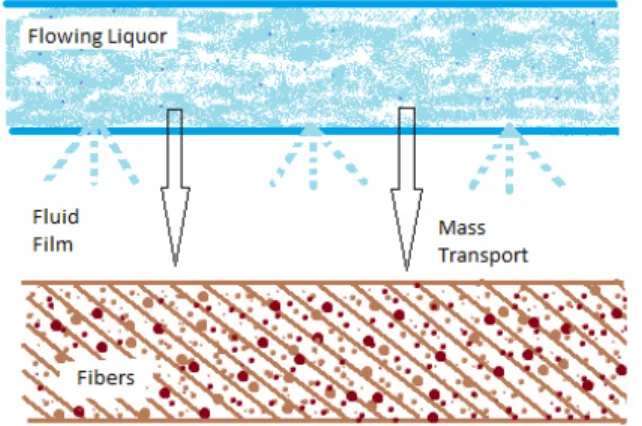
The packed bed, in the present study, is divided into two zones, namely a zone of flowing liquor and the zone of porous material. The packed bed is com-posed of unbleached Kraft pulp fibers having cy-lindrical geometry. The schematic representation of pulp fibers is given in Figure 1.
Figure 1: Schematic representation of fibers. Flow of fluid through the bed is represented by the external fluid concentration c(x,t). intraparticle and interparticle solute concentrations are repre-sented by n(r,x,t) and q(r,x,t), respectively. Particle and bed porosities are described by βand ε, respec-tively. Movement of solute within particle pores is defined by Fick’s law. The representation of different zones of the packed bed is given in Figure 2.
Figure 2: Schematic representation of different zones.
Properties of the Mathematical Model
The proposed model is based on certain features which are discussed below:
a) The system is isothermal and the bed is macro-scopically uniform.
Modelling of Displacement Washing of Pulp Fibers Using the Hermite Collocation Method 565
c) Pore radius and particle length are very small as compared to the axial distance.
d) The dispersion in the fluid is described by an axial dispersion coefficient and diffusion in particles is described by an intraparticle diffusion coefficient and both are independent of axial distance, pore ra-dius and solute concentration.
e) The adsorption equilibrium between interparti-cle and intrapartiinterparti-cle solute concentrations is assumed to be Langmuir.
f) The average solute concentration is defined
over the bed cross section.
Model for the Particle Phase
The diffusion equation describing the movement of solute within particle pores as defined by Pellett (1966), is given by:
2
2 1 F
w w w
D
r r t
r
⎛∂ + ∂ ⎞=∂
⎜ ⎟
⎜∂ ∂ ⎟ ∂
⎝ ⎠ (1)
where w is the local intraparticle solute concentration and does not distinguish between the solute adsorbed on the particle surface and the solute within the parti-cle pores. To distinguish between these two, the sur-face diffusion effects are assumed to be negligible. The transport of solute within the particles is effec-tively described by a diffusion equation involving both the concentration of solute adsorbed on the par-ticle surface and the intrapore solute concentration. The driving force for diffusion is assumed to be the intrapore concentration gradient and therefore the intraparticle diffusion equation takes the following form:
2
2
1 (1 )
F
q q q n
D
r r t t
r
⎛∂ + ∂ ⎞=∂ + − ∂
⎜ ⎟
⎜∂ ∂ ⎟ ∂ ∂
⎝ ⎠
β
β (2)
The local solute concentration applies to
par-ticles at any radial distance ‘r’, which gives
(1 )
w=β q+ −β n, and local equilibrium is assumed to prevail in the individual intraparticle pores.
Adsorption Isotherms
Immense literature is available for a linear ad-sorption isotherm (Sherman, 1964; Pellett, 1966; Neretnieks, 1974; Perron & Lebeau, 1977; Rasmuson & Neretnieks, 1980; Kukreja et al., 1995; Potůček, 1997; Potůček & Pulcer, 2004). This is due to the fact that a linear adsorption isotherm linearises the
differential equation describing the behavior of fluid flow and condenses the mathematical complexities. Crotogino et al. (1987), Trinh et al. (1989), Al-Jabari
et al. (1994) are among the prominent names to
fol-low the study of the Langmuir adsorption isotherm. However, these authors discussed the bulk fluid phase only. In the present study, the intrapore solute concentration and the concentration of solute adsorbed on the particle surface are related by a Langmuir ad-sorption isotherm in the particle phase. The mass balance equation for the adsorption isotherm is:
1 ( 0 ) 2
F
n q
k N n k n
t C
∂ = − −
∂ (3)
Model for the Bulk Fluid
The transport phenomenon in the porous media with a bed porosity ε is described by a one-dimen-sional axial dispersion model involving an axial dis-persion coefficient (Rasmuson & Neretnieks, 1980). The mass balance equation for the bulk fluid is:
2
2 (1 )
L
c c c q
D u
x t t
x
Δ
∂ = ∂ + ∂ + − ∂
∂ ∂ ∂
∂
ε ε ε ε (4)
where qΔis defined as the volume average concentra-tion in the particles. To correlate the intrapore solute concentration and the bulk fluid concentration, it is necessary to define a relation between these two in terms of axial distance.
2 0 2
( , , ) R
q q r x t r dr
R
Δ
=
∫
(5)Rasmuson & Neretnieks (1980) and Raghvan & Ruthven (1983) have related the particle phase and bulk fluid phase by defining the condition at the particle boundary. Therefore, Eq. (5) reduces to the following form:
(
)
2 q t
f
r R k
c q
KR
Δ
=
∂ =∂ β − (6)
Using Eq. (6) in Eq. (4), the latter takes the form:
2
2
1
2 f ( | )
L r R
k
c c c
D u c q
t x x KR =
∂ = ∂ − ∂ − ⎛ − ⎞ −
⎜ ⎟
∂ ∂ ∂ ⎝ ⎠
β ε
Brazilian Journal of Chemical Engineering
Initial and Boundary Conditions
The concentration gradient is assumed to be zero at the centre of the particle, i.e.,
0
q r
∂ =
∂ , at r = 0 and t > 0 (8)
It is assumed that external mass transfer resis-tance exists at r = R and mass transfer to the particle surface is controlled by the film resistance mass transfer coefficient.
(
)
f
F r R
k q
D q c
r K =
∂ ⎛ ⎞
− ⎜ ⎟= −
∂ ⎝ ⎠
β
at r = R and t > 0 (9)
It signifies the relation between Eq. (6) and Eq. (9). At the inlet and creek of the bed, Danckwart’s boundary conditions were applied.
0 L
c
uc D
x
∂
− =
∂ at x = 0 (10)
0
c x
∂ =
∂ at x = L and t > 0 (11)
Initially, c = q = C0 and n = N0 (12)
Rearranging and introducing dimensionless vari-ables given in the nomenclature, the mathematical Equations (2), (3) and Equations (7) to (12) can be converted into the following form:
2
1 2
1
Q Q Q N
N
∂ + ∂ =∂ + ∂
∂ ∂ ∂
∂η η η τ μ τ (13)
* 1( 1 (1 ) )
N
P C Q N k N
∂ = − −
∂τ (14)
2
1
2 ( | )
C Bi C C
Bi Bi C Q
Pe =
∂ = ∂ − ∂ − −
∂τ ψ ∂ξ ψ ∂ξ θ η (15)
0
Q
∂ =
∂η , at η = 0 and τ >0 (16)
1
( | )
Q
Bi C Q =
∂ = −
∂η η , at η=1 andτ >0 (17)
1
0
C C
Pe
∂
− ∂ξ = , at ξ = 0 andτ>0 (18)
0
C
∂ =
∂ξ , at ξ = 1 andτ >0 (19)
( )
( )
Initially, 1,
for all 0,1 and 0,1
C Q N
h
= = =
ξ (20)
HERMITE COLLOCATION METHOD
Orthogonal collocation is one of the weighted re-sidual methods used to solve the system of boundary value problems. In this technique the residual is set equal to zero at collocation points. For a stiff system of equations, the method of orthogonal collocation does not give good results for small values of the parameters. To overcome this problem, Carey & Finlayson (1975) proposed the conjunction of finite elements with the orthogonal collocation method, termed as orthogonal collocation on finite elements (OCFE). In this technique, the trial function is ap-proximated by using Lagrangian interpolating poly-nomials as base functions. With Lagrangian interpo-lating polynomials as base functions, an additional condition of continuity has to be imposed to make the approximating function continuous at the node points. To overcome this problem, the Hermite collo-cation method (HCM) was proposed, which is the combination of Hermite interpolating polynomials and the orthogonal collocation technique. In the Her-mite collocation method cubic HerHer-mite interpolating polynomials are used as base functions to approxi-mate the trial function (Dyksen & Lynch, 2000; Lang & Sloan, 2002; Jung, 2003; Liu et al., 2005; Ma et
al., 2006; Finden, 2007; Mazroui et al., 2007; Han,
2009; Ricciardi & Brill, 2009; Gülsu et al., 2011; Yalçinbaşet al., 2011; Orsini et al., 2011). To apply the collocation technique, the residual is set equal to zero at the collocation points. In Hermite interpolat-ing polynomials, the additional condition of continu-ity at node points is not required due to the structure of Hermite interpolating polynomials, as the Hermite interpolating polynomials possess C1 continuity. Therefore, the Hermite collocation method has the property to transform the mixed collocation method into an interior collocation method, which reduces the number of collocation equations.
Modelling of Displacement Washing of Pulp Fibers Using the Hermite Collocation Method 567 2 3 1 1 1 1 1 2 3 1 1 1 1 1 3 2 ( ) 3 2 0 elsewhere j j j j
j j j j
j j j
j j
j j j j
P
ξ ξ ξ ξ ξ ξ ξ
ξ ξ ξ ξ
ξ ξ ξ ξ ξ ξ ξ ξ
ξ ξ ξ ξ
+ + + + + − − − − − ⎧ ⎛ − ⎞ ⎛ − ⎞ ⎪ ⎜⎜ ⎟⎟ − ⎜⎜ ⎟⎟ ≤ ≤ ⎪ ⎝ − ⎠ ⎝ − ⎠ ⎪ ⎪⎪ ⎛ ⎞ ⎛ ⎞ =⎨ − − − ≤ ≤ ⎜ ⎟ ⎜ ⎟ ⎪ ⎜⎝ − ⎟⎠ ⎜⎝ − ⎟⎠ ⎪ ⎪ ⎪ ⎪⎩ (21)
(
) (
)
(
)
(
) (
)
(
)
2 3 1 1 1 2 1 1 2 3 1 1 1 2 1 1 ( ) 0 elsewhere j j j jj j j j
j j j
j j
j j j j
P
ξ ξ ξ ξ
ξ ξ ξ
ξ ξ ξ ξ
ξ ξ ξ ξ ξ
ξ ξ ξ
ξ ξ ξ ξ
+ + + + + − − − − − ⎧ − − ⎪ − ≤ ≤ ⎪ − − ⎪ ⎪⎪ =⎨− − − + ≤ ≤ ⎪ − − ⎪ ⎪ ⎪ ⎪⎩ (22)
The piecewise cubic Hermite basis functions are designed such that:
( )
j i ji
P ξ =δ , '(Pj ξi)=0, Pj( )ξi =0,Pj'( )ξi =δji.
Orthogonal collocation is applied within each sub-domain in the radial and axial direction by intro-ducing new variables η* and ζ , respectively, in such a way that
h
−
= γ
γ ξ ξ
ζ , where hγ =ξγ+1−ξγ
such that ζ= 0 when ξ ξ= γand ζ=1 when ξ ξ= γ+1,
and *
h
η η η = − A
A
, where hA=ηA+1−ηAsuch that η*=
0 when η η= Aand η*=1 when
1
+
= A
η η .
After rearranging the terms, Pj( )ξ and Pj( )ξ take the following form (Finlayson, 1980):
2 3 1 2 2 2 3 2 4
( ) 1 3 2
( ) ( 1)
( ) (3 2 )
( ) ( 1)
H H h H H h = − + = − = − = − γ γ
ζ ζ ζ
ζ ζ ζ
ζ ζ ζ
ζ ζ ζ
(23)
Therefore, the approximating function for Cγ( , )ζ τ
can be defined as
4
1
( , ) i ( ) i( )
i
C c H
=
=
∑
γ ζ τ γ τ ζ , where
the 'ciγ s are continuous functions of τ. Similarly, the
approximating functions for Q (ℓ,γ)(η,ζ,τ) and N (ℓ,γ)
(η,ζ,τ) can be defined in both the radial and axial directions. The structure of the (γ −1)th, γth and
th
(γ +1) elements in the axial domain for Hermite collocation is defined in Figure 3.
cγ-1
1 cγ-12 cγ-13 cγ-14 cγ+11 cγ+12 cγ+13 cγ+14 cγ1 cγ2 cγ3 cγ4
( -1)thElement ( +1)thElement thElement
cγ-1
1 cγ-12 cγ-13 cγ-14 cγ-1
1 cγ-12 cγ-13 cγ-14 ccγ+1γ+111 ccγ+1γ+122 ccγ+1γ+133 ccγ+1γ+144 cγ1 cγ2 cγ3 cγ4
cγ1 cγ2 cγ3 cγ4
( -1)thElement ( +1)thElement thElement
Figure 3: Structure of the (γ −1)th, γth and (γ +1)th elements in Hermite collocation.
COLLOCATION POINTS
Choice of the collocation points is the basis of the collocation technique. These are chosen in such a way to keep the error minimum. Therefore, the inte-rior collocation points in both the axial and radial direction are taken to be the roots of the shifted Legendre polynomial. The collocation points are
taken to be 2 1 1
2 2 3
= −
ζ and 3 1 1
2 2 3
= +
ζ with 0
and 1 as boundary points by transforming the domain [-1,1] of a shifted Legendre polynomial of order 2 onto [0,1].
As given in the previous section, substituting 4
1
( , ) i ( ) i( )
i
C c H
=
=
∑
γ ζ τ γ τ ζ ,
4
, ,
1
( , , ) i i( )
i
Q q H
=
=
∑
Aγ η ζ τ Aγ η ,
4
, ,
1
( , , ) i i( )
i
N n H
=
=
∑
Aγ η ζ τ Aγ η , gives
1 1 1 2 1 ( ) ( ) c c Pe =
τ τ , 2
4 ( ) 0
s
c τ = and q2(1, )γ ( )τ =0,
1 1 4 ( , ) ( , ) 4 3 1 ( ) [ ( ) ( )] s s i ji i
q Bi c H q
=
=
∑
−γ τ γ τ γ τ in the axial
Brazilian Journal of Chemical Engineering
4 ( , ) 4 4
( , ) ( , )
2 *
1 1 1
4 4 4
( , ) ( , ) * ( , ) 1 1 1
1 1
1
1
2 for all, 1, 2,..., , 1, 2,...
1 1
,
1 i
ji i ji i ji
j
i i i
i ji i ji i ji
i i i
dq
H q B q A
d h h
N P C q H n H n
s
k
s
H
γ
γ γ
γ γ γ
τ η
μ
γ
= = =
= = =
= +
⎛ ⎛ ⎞⎛ ⎞ ⎞
⎜ ⎟
− ⎜ ⎜⎜ ⎟⎜⎟⎜ − ⎟⎟− ⎟
⎝ ⎠⎝ ⎠
= =
⎝ ⎠
∑
∑
∑
∑
∑
∑
A
A A
A A
A A A
A
(24)
4 ( , ) 4 4 4
( , ) ( , ) * ( , ) 1 1
1 1 1 1
2 1
for all, 1, 2,..., , 1, 2,.. ,
1
. i
ji i ji i ji i ji
i i i i
dn
H P C q H n H k n H
s s
d
γ
γ γ γ
γ τ
= = = =
⎛ ⎛ ⎞⎛ ⎞ ⎞
⎜ ⎟
= ⎜ ⎜⎜ ⎟⎜⎟⎜ − ⎟⎟− ⎟
⎝ ⎠⎝ ⎠
⎝ ⎠
= =
∑
A∑
A∑
A∑
AA
(25)
4 ( ) 4 4 4 4
( ) ( ) ( ) ( , )
1 2
1 1 1
1
1 1
2 for all, 1, 2,..., , 1, 2,...,
m i
ji ji
ji i i i ji i i
i i i i i
dc Bi Bi
H c B c A Bi c H q H
d Pe h h
s s
γ γ γ γ γ
γ γ
ψ ψ θ
γ τ
= = = = =
⎛ ⎞
= − − ⎜⎜ − ⎟⎟
⎝ ⎠
= =
∑
∑
∑
∑
∑
A
(26)
where Bji and Aji are discretization matrices for the second- and first-order derivatives, respectively, in the radial domain and BjiandAji are discretization matrices for the second- and first-order derivatives, respectively, in the axial domain. The resulting sys-tem of differential equations can be put into the ma-trix form asH C' = M C, where H is the matrix of Hermite functions, Cis the matrix of collocation functions and C'is the matrix of the derivative of these collocation functions with respect to time and M is the coefficient matrix.
After application of HCM, for 5 elements in the radial domain and varying elements in the axial do-main, ‘46s2’ number of differential equations appear, where s2 is the number of elements in the axial do-main. This system of differential equations is solved using MATLAB with the ‘ode15s’ system solver, which uses the backward differentiation formula to
solve the system of differential equations.
STABILITY ANALYSIS
The test of every numerical technique lies in how stable it is or how fast it converges. In present study, the stability analysis was made on the basis of the L2-norm and L∞-norm. In Table 1 to Table 4, the L2
-norm and L∞-norm are presented for different values of Peclet number Pe and Biot number Bi at different time intervals. The average bed porosity ε and di-mensionless parameter ψ are taken to be 0.6314 and 0.1, respectively. The values in Table 1 to Table 4 are found to be stable after 10 elements in the axial
do-main. However, the L∞-norm is observed to be
higher than the L2-norm, but the stability in the
re-sults can be better judged by the L2- norm as
com-pared to the L∞- norm.
Table 1: L2-norm and L∞-norm for Pe=5, Bi=4.5.
τ (-) 2 elements 5 elements 10 elements 12 elements
||C||2 ||C||∞ ||C||2 ||C||∞ ||C||2 ||C||∞ ||C||2 ||C||∞
0 1.000 1.000 1.000 1.000 1.000 1.000 1.000 1.000
0.50 0.935 1.035 0.920 1.363 0.903 1.502 0.900 1.523
1.00 0.772 0.927 0.791 1.045 0.787 1.100 0.787 1.116
1.25 0.696 0.877 0.727 0.964 0.729 0.994 0.728 1.002
Modelling of Displacement Washing of Pulp Fibers Using the Hermite Collocation Method 569
Table 2: L2-norm and L∞-norm for Pe=7, Bi=5.5.
τ (-) 2 elements 5 elements 10 elements 12 elements
||C||2 ||C||∞ ||C||2 ||C||∞ ||C||2 ||C||∞ ||C||2 ||C||∞
0 1.000 1.000 1.000 1.000 1.000 1.000 1.000 1.000
0.50 0.935 1.083 0.945 1.496 0.940 1.568 0.938 1.604
1.00 0.732 0.999 0.782 1.120 0.786 1.146 0.786 1.161
1.25 0.636 0.892 0.702 0.987 0.710 1.028 0.711 1.038
1.75 0.458 0.655 0.539 0.828 0.558 0.854 0.556 0.857
Table 3: L2-norm and L∞-norm for Pe=10, Bi=6.7.
τ (-) 2 elements 5 elements 10 elements 12 elements
||C||2 ||C||∞ ||C||2 ||C||∞ ||C||2 ||C||∞ ||C||2 ||C||∞
0 1.000 1.000 1.000 1.000 1.000 1.000 1.000 1.000
0.50 0.923 1.232 0.956 1.541 0.960 1.663 0.960 1.675
1.00 0.666 0.980 0.758 1.127 0.769 1.195 0.770 1.200
1.25 0.536 0.783 0.656 1.050 0.673 1.073 0.674 1.078
1.75 0.320 0.440 0.450 0.790 0.473 0.846 0.476 0.852
Table 4: L2-norm and L∞-norm for Pe=15, Bi=7.5.
τ (-) 2 elements 5 elements 10 elements 12 elements
||C||2 ||C||∞ ||C||2 ||C||∞ ||C||2 ||C||∞ ||C||2 ||C||∞
0 1.000 1.000 1.000 1.000 1.000 1.000 1.000 1.000
0.50 0.938 1.391 0.981 1.665 0.992 1.836 0.993 1.850
1.00 0.609 0.907 0.761 1.286 0.778 1.302 0.780 1.311
1.25 0.438 0.616 0.637 1.095 0.666 1.174 0.669 1.182
1.75 0.200 0.359 0.385 0.823 0.425 0.890 0.429 0.893
EXPERIMENTAL
Displacement washing experiments simulated un-der the laboratory conditions were performed in a cylindrical glass cell with inside diameter of 35 mm under constant bed height of 30 mm. The fiber pulp bed occupied the volume between the permeable sep-tum and a piston, covered with 45 mesh screens to prevent fiber losses from the bed.
Pulp beds were formed from a dilute suspension of unbeaten unbleached Kraft pulp in black liquor. Pulp was obtained from a blend of softwoods con-taining approximately ¾ spruce and ¼ pine. After compressing to the desired thickness of 30 mm, the consistency, i.e., mass concentration of moisture-free pulp fibers in the bed was about 12%. In order to characterise the pulp fibers used in the experiments, physical properties of Kraft pulp were determined. The Schopper-Riegler freeness had a value of 13.5°SR. The degree of delignification of the pulp was expressed by the kappa number of about 32. Using the Kajaani FS-100 instrument, the mean length of the fibers was also measured. The weighted average length was 3.35 mm, while the numerical average length was 1.46 mm. The specific surface of fibers having a coarseness of 0.15 mg m-1 was 733 m2 kg-1.
Distilled water was used as wash liquid and was distributed uniformly through the piston to the top of bed at the start of the washing experiment. At the same time, the displaced liquor was collected at at-mospheric pressure from the bottom of the bed via
the septum. The washing effluent was sampled at different time intervals until the effluent was colour-less. Samples of the washing effluent leaving the pulp bed were analysed for alkali lignin using an ultraviolet spectrophotometer operating at a wave-length of 295 nm. In Table 5, the input values for three runs of experiments are given. Displacement washing experiments with composition of pulp fi-bers, including washing equipment, were described in detail in Arora & Potůček (2012).
Table 5: Experimental data of pulp fibers.
Parameter Value Unit
Pe 7.921-10.651 -
ε 0.6075-0.6314 -
u (0.1300-0.2071)×10-3 m/s
Consistency 11.737-12.303 %
DL (0.611-1.145)×10-6 m2/s
β 0.7246 -
L 30×10-3 m
Brazilian Journal of Chemical Engineering
RESULTS AND DISCUSSION
It can be observed from Table 1 to Table 4 that stability occurs after 10 elements in the axial do-main. Therefore, the theoretical effect of different parameters on the exit solute concentration will be discussed for 5 elements in the radial domain and 10 elements in the axial domain.
Effect of Peclet Number (Pe)
In Figure 4, the theoretical effect of Peclet num-ber is shown on the exit solute concentration for
Bi = 5 and ε = 0.6314. It can be observed from this figure that, as the value of Peclet number increases,
i.e., for Pe ≥ 20, solution profiles converge rapidly to the steady-state condition and follow a Gaussian shape curve. However, for small values of Peclet number, i.e., Pe = 5, solution profiles take a long time to converge to a steady-state condition. This is due to the fact that, for small values of Pe, the axial disper-sion coefficient (DL) is large. It causes more back mixing and, as a result, fewer impurities are washed out and a long time in the washing operation is re-quired. Therefore, high Pe is preferred for better washing operations at small intervals of time. For
Pe = 20 and Pe = 30, no considerable effect is ob-served on solution profiles. It authenticates the fact that better washing operations can be achieved for Pe
≤ 30 (Al-Jabari et al., 1994; Arora et al., 2006).
Figure 4: Behaviour of the solution profile for dif-ferent values of Pe with Bi = 5 and ε = 0.6314.
Effect of Biot Number (Bi)
Biot number (Bi) signifies the mass transfer resis-tances inside and on the surface of the particle. Theo-retical effects of Biot number on the solution profiles are shown in Figure 5 for Pe = 10 and ε = 0.6314. For small values of Biot number, i.e., Bi = 5, solution profiles take a long time to converge to the
steady-state condition as compared to large values of Biot number, i.e., Bi = 15, where the solution profile con-verges for τ nearly equal to 3. This is due to the fact that, for high Bi, the mass transfer rate increases, resulting in more removal of impurities adsorbed on the particle surface and hence better washing opera-tions can be achieved.
Figure 5: Behaviour of the solution profile for dif-ferent values of Bi with Pe = 10 and ε = 0.6314.
Effect of the Dimensionless Parameter ψ
The effect of pore radius of the particle, film resistance mass transfer coefficient and interstitial velocity can be observed effectively by studying the
effect of the dimensionless parameter ψ on the
solution profiles. In Figure 6 the theoretical effect of
ψis shown for Pe = 10, Bi = 6.7 and ε = 0.6314.
Figure 6: Behaviour of the solution profile for dif-ferent values of the dimensionless parameter ψ for
Pe = 10, Bi = 6.7 and ε = 0.6314.
in-Modelling of Displacement Washing of Pulp Fibers Using the Hermite Collocation Method 571
creases the diffusion in the particle pores, resulting in better removal of impurities adsorbed on the particle surface and hence better washing operations can be attained. For ψ> 0.5 no significant effect can be analysed on the solution profiles.
Effect of Bed Porosity (ε)
The packed bed porosity, εis the most significant and perceptive factor which affects the solution pro-files extensively. As the value of bed porosity in-creases, permeability increases causing the amount of solute removed from interparticle voids by the convective mechanism to increase, and the washing process runs very rapidly. The effect of bed porosity
ε for Pe = 10 and Bi = 6.7, is shown in Figure 7. It can be easily observed from the figure that the solu-tion profiles converge to the steady-state condisolu-tion more rapidly for ε = 0.8120 as compared to ε = 0.5561.
Figure 7: Behaviour of the solution profile for dif-ferent values of ε with Pe = 10 and Bi = 6.7.
Wash Yield (WYτ=1)
The most significant solute removal parameter used in the industry is wash yield. It is the proportion of dissolved solids removed relative to the dissolved solids entering with the unwashed pulp. If the solute is split in a similar portion as the fluid, it is easy to analyse how much solute is left in the thickened pulp. Wash yield defined for τ = 1 can be calculated using the following formula (Potůček, 1997):
1
0 1
0
e
e C d
WY
C d
= =
∫
∫
τ τ
τ
τ
(27)
Wash yield for Pe = 9, Bi = 6 and ε = 0.6075 was calculated at different time intervals for 5 elements in the radial domain and varying elements in the axial domain. Values of WY are given in Table 6. It is observed from this table that wash yield at any time lies within the range varying from 0.7 to 0.8 which is less than nearly seventy times the initial solute con-centration. As time increases from τ = 5, no consider-able effect is observed and the values of WYτ=1
re-main stable. For pulp fibers, the influence of Peclet number on wash yield can be linked by Equation
(28) given by Potůček (2005), which agrees well
with the values given in Table 6.
0.040
1 0.72
WYτ= = Pe (28)
Table 6: WY τ=1 for different elements of the axial domain and at varying time periods.
τ (-) 2 elements 5 elements 10 elements 12 elements
2 0.7834 0.7680 0.7604 0.7592
3 0.7566 0.7394 0.7306 0.7294
4 0.7532 0.7355 0.7266 0.7252
5 0.7528 0.7349 0.7260 0.7247
COMPARISON OF EXPERIMENTAL AND NUMERICAL VALUES
Theoretically, one can vary a single parameter keep-ing the other parameters constant. However, practi-cally, it is not possible to vary only a single parame-ter. As bed porosity changes, the pore radius of the particle, interstitial velocity and permeability vary, which varies the axial dispersion and intraparticle dif-fusion coefficient and, therefore, the Peclet number and Biot number also vary. In Figure 8 the behaviour of the solution profiles is shown for different values of Pe, Bi and ε. Although the range of bed porosity does not vary greatly, the solution profiles converge rapidly for Pe = 10.651 and Bi = 6.7 as compared to
Pe = 7.921 and Bi = 5.5. It reflects the fact that, with the increase in Biot number, the pore radius of parti-cles increases, which gives better washing results.
In Table 7, a comparison between experimental and numerical values is shown for different values of
Pe, Bi and ε in terms of relative error:
Relative error exp num
exp
C C
C
−
= (29)
Brazilian Journal of Chemical Engineering
Figure 8: Behaviour of the solution profiles for different values of Pe, Bi and ε.
Table 7: Comparison of Experimental and Numerical values.
Pe=7.921, Bi=5.5,ε=0.6314 Pe=9.230, Bi=6,ε=0.6075 Pe=10.651, Bi=6.7,ε=0.6195
Experimental Numerical Relative
Error
Experimental Numerical Relative
Error
Experimental Numerical Relative
Error
1.0000 1.00000 0.0000 1.00000 1.0000 0.0000 1.0000 1.00000 0.0000 1.0000 1.00048 4.8000×10⁻⁴ 9.6737×10⁻¹ 9.6929×10⁻¹ 1.9766×10⁻³ 1.0000 1.00157 1.5700×10⁻³ 9.7173×10⁻¹ 9.7029×10⁻¹ 1.4838×10⁻³ 9.3008×10⁻¹ 9.3093×10⁻¹ 9.1202×10⁻⁴ 1.0000 1.00087 8.7000×10⁻⁴ 8.8734×10⁻¹ 8.8681×10⁻¹ 6.0321×10⁻⁴ 9.0763×10⁻¹ 9.0996×10⁻¹ 2.5747×10⁻³ 9.6433×10⁻¹ 9.6509×10⁻¹ 7.8795×10⁻⁴ 7.1077×10⁻¹ 7.1074×10⁻¹ 4.3998×10⁻⁵ 6.4407×10⁻¹ 6.4714×10⁻¹ 4.7762×10⁻³ 7.9303×10⁻¹ 7.9107×10⁻¹ 2.4727×10⁻³ 6.1286×10⁻¹ 6.1219×10⁻¹ 1.1040×10⁻³ 5.5085×10⁻¹ 5.5074×10⁻¹ 1.9326×10⁻⁴ 7.7146×10⁻¹ 7.7267×10⁻¹ 1.5696×10⁻³ 5.6985×10⁻¹ 5.6967×10⁻¹ 3.2013×10⁻⁴ 4.3051×10⁻¹ 4.3232×10⁻¹ 4.2148×10⁻³ 6.5989×10⁻¹ 6.6091×10⁻¹ 1.5424×10⁻³ 9.2175×10⁻² 9.2648×10⁻² 5.1268×10⁻³ 1.2712×10⁻² 1.2817×10⁻² 8.2313×10⁻³ 6.5948×10⁻² 6.5857×10⁻² 1.3774×10⁻³ 3.2773×10⁻² 3.2812×10⁻² 1.1700×10⁻³ 8.0508×10⁻³ 8.1164×10⁻³ 8.1460×10⁻³ 1.9909×10⁻² 1.9781×10⁻² 6.4219×10⁻³ 2.6628×10⁻³ 2.6742×10⁻³ 4.2687×10⁻³ 1.4407×10⁻³ 1.4476×10⁻³ 4.7769×10⁻³ 2.3642×10⁻³ 2.3717×10⁻³ 3.2002×10⁻³ 1.1471×10⁻³ 1.1368×10⁻³ 8.9802×10⁻³ 8.4746×10⁻⁴ 8.4127×10⁻⁴ 7.2967×10⁻³ 1.1199×10⁻³ 1.1133×10⁻³ 5.8375×10⁻³ 6.9644×10⁻⁴ 6.9108×10⁻⁴ 7.6962×10⁻³ 5.9322×10⁻⁴ 5.8904×10⁻⁴ 7.0502×10⁻³ 6.6363×10⁻⁴ 6.6479×10⁻⁴ 1.7630×10⁻³ 5.3257×10⁻⁴ 5.3132×10⁻⁴ 2.3370×10⁻³ 4.6610×10⁻⁴ 4.7017×10⁻⁴ 8.7198×10⁻³ 4.9772×10⁻⁴ 4.9464×10⁻⁴ 6.1858×10⁻³
Displacement Ratio (DR)
Displacement ratio is the most perceptive factor in the washing theory. It is calculated from the aver-age solute concentration of the solute using the fol-lowing formula:
1 av
DR= −C (30)
In Figure 9, a comparison has been made for the displacement ratio calculated for different values of
Pe, Bi and ε. It is observed from this figure that, with the increase in the value of Pe, Bi and ε, the solution profiles for DR converge more rapidly as compared to small values of Pe, Bi and ε. For different values of Pe, Bi and ε, the solution profiles converge at almost the similar times. This is because the bed porosity lies in same range in the three washing runs
(Arora & Potůček, 2012). However, the solution pro-file converges slightly faster for Pe = 10.651 as com-pared to other solution profiles.
Figure 9: Behaviour of DR for different values of
Modelling of Displacement Washing of Pulp Fibers Using the Hermite Collocation Method 573
CONCLUSIONS
A mathematical model for the displacement washing process was presented and solved using HCM. Numerical results were compared with the experimental ones of a washing cell for different values of displacement washing parameters. It can be concluded from all the experimental and theoretical findings that the proposed mathematical model agrees fairly well with the experimental data, in view of significant aspects of dispersion, diffusion and different porosities. Comparison of numerical and experimental values presented in the tables and graphs validate this information.
ACKNOWLEDGEMENT
Dr. Shelly Arora is thankful to UGC for providing financial assistance in the form of the major research project F. No. 41-786/2012(SR). Ms. Inderpreet Kaur is thankful to DST for providing a INSPIRE fellow-ship. Authors are thankful to reviewers for their valu-able comments.
NOMENCLATURE
Bi Biot number, dimensionless
(=kf R/KDF)
c concentration of solute in the liquor (kg/m3)
C dimensionless concentration (=c/C0)
C0 solute concentration in the vat (kg/m3)
C1 dimensionless parameter (=C0/CF)
Cav average solute concentration, dimensionless
Ce exit solute concentration, dimensionless
CF fiber consistency (kg/m3)
DF intrafiber diffusion coefficient (m2/s)
DL axial dispersion coefficient (m2/s)
DR Displacement Ratio, dimensionless
K volume equilibrium constant, dimensionless
k* mass transfer coefficient, dimensionless
(=k2/k1)
k1, k2 mass transfer coefficient (1/s)
kf film mass transfer coefficient (m/s)
L thickness of the bed (m)
n concentration of solute adsorbed on the
fibers (kg/m3)
N dimensionless concentration of solute
adsorbed on fibers (=n/N0)
N0 initial concentration of solute adsorbed on the fibers (kg/m3)
N1 dimensionless parameter (=N0 /C0)
P1 dimensionless parameter (=k1R
2 / DF)
Pe Peclet number, dimensionless (=uL/DL)
Q dimensionless pore liquid concentration
(=q/C0)
q pore liquid concentration (kg/m3)
R fiber radius(m)
r radial position in particle (m)
t time (s)
u interstitial velocity through bed (m/s)
WY wash yield, dimensionless
x distance from point of introduction of
solvent (m)
Greek Symbols
β particle porosity, dimensionless
ε porosity of cake, dimensionless
η dimensionless radial coordinate (= r/R)
θ 2(1−ε ε) /
μ (1-β)/β (dimensionless)
ξ dimensionless axial coordinate (= x/L)
τ dimensionless time (= t DF/R2)
ψ dimensionless parameter (=KRu/kfβ L)
REFERENCES
Adomaitis, R. A. and Lin, Y., A collocation/quadra-ture-based Sturm-Liouville problem solver. Applied Mathematics and Computation, 110, pp. 205-223 (2000).
Al-Jabari, M., van Heiningen, A. R. P. and van De Ven, T. G. M., Modelling the flow and the deposi-tion of fillers in packed beds of pulp fibers. Jour-nal of Pulp and Paper Science, 20(9), pp. J249-J253 (1994).
Aminikhah, H., The combined Laplace transform and the new homotopy perturbation methods for stiff systems of ODEs. Applied Mathematical Modelling, 36, pp. 3638-3644 (2012).
Arora, S., Dhaliwal, S. S. and Kukreja, V. K., Solu-tion of two point boundary value problems using orthogonal collocation on finite elements. Ap-plied Mathematics and Computation, 171, pp. 358-370 (2005).
Arora, S., Dhaliwal, S. S. and Kukreja, V. K., Simu-lation of washing of packed bed of porous parti-cles by orthogonal collocation on finite elements. Computers and Chemical Engineering, 30, pp. 1054-1060 (2006).
Arora, S., Dhaliwal, S. S. and Kukreja, V. K., Mathe-matical modelling of the washing zone of an in-dustrial rotary vacuum washer. Indian Journal of Chemical Technology, 15, pp. 332-340 (2008). Arora, S. and Potůček, F., Verification of
Brazilian Journal of Chemical Engineering fibres. Indian Journal of Chemical Technology,
19, pp. 140-148 (2012).
Bhrawy, A. H. and El-Soubhy, S. I., Jacobi spectral Galerkin method for the integrated forms of sec-ond-order differential equations. Applied Mathe-matics and Computation, 217, pp. 2684-2697 (2010).
Brenner, H., The diffusion model of longitudinal mixing in beds of finite length: Numerical values. Chemical Engineering Science, 17, pp. 229-243 (1962).
Carey, G. F. and Finlayson, B. A., Orthogonal collo-cation on finite elements. Chemical Engineering Science, 30, pp. 587-596 (1975).
Crotogino, R. H., Poirier, N. A. and Trinh, D. T., The principles of pulp washing. Tappi Journal, 70(6), pp. 95-103 (1987).
Dhawan, S., Kapoor, S. and Kumar, S., Numerical method for advection diffusion equation using FEM and B-splines. Journal of Computational Science, 3, pp. 429-437 (2012).
Dyksen, W. R. and Lynch, R. E., A new decoupling technique for the Hermite cubic collocation equa-tions arising from boundary value problems. Mathematics and Computers in Simulation, 54, pp. 359-372 (2000).
El-Daou, M. K. and Al-Matar, N. R., An improved Tau method for a class of Sturm-Liouville prob-lems. Applied Mathematics and Computation, 216, pp. 1923-1937 (2010).
Eriksson, G., Rasmuson, A. and Theliander, H., Dis-placement washing of lime mud: Tailing effects. Separations Technology, 6, pp. 201-210 (1996). Finden, W. F., Higher order approximations using
interpolation applied to collocation solutions of two-point boundary value problems. Journal of Computational and Applied Mathematics, 206, pp. 99-115 (2007).
Finlayson, B. A., Nonlinear Analysis in Chemical Engineering. McGraw-Hill, New York (1980). Grähs, L. E., Washing of cellulose fibres: Analysis of
displacement washing operation. Ph.D. Thesis, Chalmers University of Technology, Goteborg, Sweden (1974).
Gülsu, M., Yalman, H., Öztürk, Y. and Sezer, M., A new Hermite collocation method for solving dif-ferential difference equations. Applications and Applied Mathematics, 6(11), pp. 1856-1869 (2011). Han, X., A degree by degree recursive construction
of Hermite spline interpolants. Journal of Compu-tational and Applied Mathematics, 225, pp. 113-123 (2009).
Han, C. D., Washing theory of the porous structure of aggregated materials. Chemical Engineering Science, 22, pp. 837-846 (1967).
Jung, H. S., L∞ Convergence of interpolation and as-sociated product integration for exponential weights. Journal of Approximation Theory, 120, pp. 217-241 (2003).
Kadalbajoo, M. K., Yadav, A. S. and Kumar, D., Comparative study of singularly perturbed two-point BVP’s via: Fitted mesh finite difference method, B-spline collocation method and finite element method. Applied Mathematics and Com-putation, 204, pp. 713-725 (2008).
Khuri, S. A. and Sayfy, A., Spline collocation ap-proach for the numerical solution of a generalized system of second-order boundary-value problems. Applied Mathematical Sciences, 3(45), pp. 2227-2239 (2009).
Kukreja, V. K., Ray, A. K., Singh, V. K. and Rao, N. J., A Mathematical model for pulp washing in different zones of a rotary vacuum filter. Indian Chemical Engineer Section A, 37(3), pp. 113-124 (1995). Lang, A. W. and Sloan, D. M., Hermite collocation
solution of near-singular problems using numeri-cal coordinate transformations based on adaptiv-ity. Journal of Computational and Applied Mathe-matics, 140, pp. 499-520 (2002).
Liao, H. T. and Shiau, C. Y., Analytic solution to an axial dispersion model for the fixed bed adsorber. American Institute of Chemical Engineers, 46(6), pp. 1168-1176 (2000).
Liu, F. and Bhatia, S. K., Application of Petrov-Galerkin methods to transient boundary value problems in chemical engineering: Adsorption with steep gradients in bidisperse solids. Chemical Engineering Science, 56, pp. 3727-3735 (2001). Liu, X., Liu, G. R., Tai, K. and Lam, K. Y., Radial
point interpolation collocation method (RPICM) for partial differential equations. Computers and Mathematics with Applications, 50, pp. 1425-1442 (2005).
Ma, Z. and Guiochon, G., Application of orthogonal collocation on finite elements in the simulation of non-linear chromatography. Computers and Chemical Engineering, 15(6), pp. 415-426 (1991). Ma, H., Sun, W. and Tang, T., Hermite spectral
meth-ods with a time-dependent scaling for parabolic equations in unbounded domains. Society for In-dustrial and Applied Mathematics, 43(1), pp. 58-75 (2006).
Mazroui, A., Sbibih, D. and Tijini, A., Recursive com-putation of bivariate Hermite splines interpolants. Applied Numerical Mathematics, 57, pp. 962-973 (2007).
Modelling of Displacement Washing of Pulp Fibers Using the Hermite Collocation Method 575
Nadukandi, P., Onate, E. and Garcia, J., A high-reso-lution Petrov-Galerkin method for the 1D convec-tion-diffusion-reaction problem. Computer Meth-ods in Applied Mechanics and Engineering, 199, pp. 525-546 (2010).
Neretnieks, I., A mathematical model for continuous countercurrent adsorption. Svensk Papperstidning-Nordisk Cellulosa, 11, pp. 407-411 (1974). Neretnieks, I., Adsorption in finite bath and
counter-current flow with systems having a non linear iso-therm. Chemical Engineering Science, 31, pp. 107-114 (1976).
Onah, S. E., Asymptotic behaviour of the Galerkin and the finite element collocation methods for a parabolic equation. Applied Mathematics and Computation, 127, pp. 207-213 (2002).
Orsini, P., Power, H. and Lees, M., The Hermite radial basis function control volume method for multi-zones problems: A non overlapping domain decomposition algorithm. Computer Methods in Applied Mechanics and Engineering, 200, pp. 477-493 (2011).
Pedas, A. and Tamme, E., Spline collocation methods for linear multi-term fractional differential equa-tions. Journal of Computational and Applied Mathematics, 236, pp. 167-176 (2011).
Pellett, G. L., Longitudinal dispersion, intraparticle diffusion and liquid-phase mass transfer during flow through multiparticle systems. Tappi Jour-nal, 49(2), pp. 75-82 (1966).
Perron, M. and Lebeau, B., A mathematical model of pulp washing on rotary drums. Pulp & Paper Can-ada, 78(3), pp. TR1-TR5 (1977).
Potůček, F., Washing of pulp fibre bed. Collection of Czechoslovak Chemical Communications, 62, pp. 626-644 (1997).
Potůček, F. and Pulcer, M., Displacement of black liquor from pulp bed. Chemical Papers, 58(6), pp. 377-381 (2004).
Potůček, F., Chemical engineering view of the pulp washing. Papir a Celulóza, 60(4), pp. 114-117 (2005).
Raghvan, N. S. and Ruthven, D. M., Numerical simu-lation of a fixed bed adsorption column by the method of orthogonal collocation. American In-stitute of Chemical Engineers, 29(6), pp. 922-925 (1983).
Rashidinia, J. and Ghasemi, M., B-Spline collocation for solution of two-point boundary value prob-lems. Journal of Computational and Applied Mathematics, 235, pp. 2325-2342 (2011).
Rasmuson, A. and Neretnieks, I., Exact solution of a model for diffusion in particles and longitudinal dispersion in packed beds. American Institute of Chemical Engineers, 26(4), pp. 686-690 (1980).
Ricciardi, K. L. and Brill, S. H., Optimal Hermite collocation applied to a one-dimensional convec-tion-diffusion equation using an adaptive hybrid optimization algorithm. International Journal of Numerical Methods for Heat and Fluid Flow, 19(7), pp. 874-893 (2009).
Shen, T. T., Xing, K. Z. and Ma, H. P., A Legendre Petrov-Galerkin method for fourth-order differen-tial equations. Computers and Mathematics with Applications, 61, pp. 8-16 (2011).
Sherman, W. R., The movement of a soluble material during the washing of a bed of packed solids. American Institute of Chemical Engineers, 10(6), pp. 855-860 (1964).
Solsvik, J. and Jakobsen, H. A., Effect of Jacobi polynomials on the numerical solution of the pel-let equation using the orthogonal collocation, Galerkin, tau and least squares methods. Com-puters and Chemical Engineering, 39, pp. 1-21 (2012).
Sporleder, F., Dorao, C. A. and Jakobsen, H. A., Simulation of chemical reactors using the least-squares spectral element method. Chemical Engi-neering Science, 65, pp. 5146-5159 (2010). Toledo, Leal, R. C. and Ruas, V., Numerical analysis
of a least squares finite element method for the time dependent advection-diffusion equation. Jour-nal of ComputatioJour-nal and Applied Mathematics, 235, pp. 3615-3631 (2011).
Trinh, D. T., Poirier, N. A., Crotogino, R. H. and Douglas, W. J. M., Displacement washing of wood pulp-an experimental study. Journal of Pulp and Paper Science, 15(1), pp. J28-J35 (1989).
Vanani, S. K. and Aminataei, A., Tau approximate solution of fractional partial differential equations. Computers and Mathematics with Applications, 62, pp. 1075-1083 (2011).
Villadsen, J. and Stewart, W. E., Solution of bound-ary value problems by orthogonal collocation. Chemical Engineering Science, 22, pp. 1483-1501 (1967).
Wu, J., Least squares methods for solving partial differential equations by using Bezier control points. Applied Mathematics and Computation, 219, pp. 3655-3663 (2012).
Yalçinbaş, S., Aynigül, M. and Sezer, M., A colloca-tion method using Hermite polynomials for ap-proximate solution of pantograph equations. Jour-nal of The Franklin Institute, 348, pp. 1128-1139 (2011).