Corporate Governance and Taxes

(1)

Corporate Governance and Taxes

André Alves Pinto Vieira 110487030

Dissertação de Mestrado em Finanças e Fiscalidade

Orientada por:

António Cerqueira Elísio Brandão

(2)

(3)

I

Perfil do candidato

André Alves Pinto Vieira, filho de Jorge Manuel da Silva Pinto Vieira e de Adelina Pereira Alves Pinto Vieira, nasceu no dia 1 de Novembro de 1990.

Natural de Vila Nova de Gaia, concluiu o Ensino Secundário no Colégio de Gaia, com média de 18 valores, em 2008, ano em que ingressou no curso de Economia na Faculdade de Economia da Universidade do Porto.

Em 2011 concluiu a licenciatura em Economia,

com média de 15 valores. Nesse mesmo ano iniciou o Mestrado em Finanças e Fiscalidade na Faculdade de Economia do Porto, no âmbito do qual apresenta esta dissertação.

(4)

II

Abstract

The purpose of this paper is to study the impact that Corporate Governance characteristics have on firms’ tax rates. The fiscal implications of stronger or weaker shareholders powers have been studied in recent literature, but most of the studies regarding that matter focus on the effect that shareholders rights have on firms’ current year’s tax related variables, considering indiscriminately firms with low, medium and high tax rates. However, we consider that stronger shareholders rights have different impacts on taxes, depending on whether firms have low or high tax rates. Thus, our paper contributes to prior research, by considering that current year’s tax rates must be considered when measuring the impact that shareholders rights have on next years’ tax rates. Thereby, we develop two different methodologies. In the first place, following prior research, our paper analyzes the relationship between Corporate Governance and current years’ tax rates, for the whole sample. Secondly, we create two firms groups – “excessive tax payers” and “tax savers” - according to their tax rates, and analyze their tax rates in the three years that follow an excessive or a low tax rate’s year. Our results support previous literature by showing that stronger shareholders rights tend to reduce current year’s tax burden. Additionally, they suggest that within the firms that have excessive tax rates in a given year, those with stronger shareholders rights have lower effective tax rates, relatively to those with weaker shareholders rights, on the following 2 years. However, within the firms that have low tax rates in a given year, there is no significant relationship between shareholders rights and next three years’ tax rates. Thus, strong shareholders rights have a significant impact on firms with high tax rates but not on firms with low tax rates. This means that current year’s tax rate is a factor that must be taken into account in future investigations that study the link between Corporate Governance and taxes.

(5)

III

Index

1. Introduction ... 1

2. Literature Review and Hypotheses Development ... 4

2.1. Literature Review ... 4

2.2. Hypotheses Development ... 6

3. Variables Description and Sample Selection ... 7

3.1. Variables Description ... 7

Tax variables ... 7

Corporate Governance variables ... 8

Firm-specific Variables ... 9

3.2. Sample Selection ... 10

4. Hypothesis 1 development ... 12

4.1. Methodology and Univariate Analysis... 12

Model 1 ... 12

Model 2 ... 15

Model 3 ... 17

4.2. Multivariate Analysis ... 20

5. Hypotheses 2 and 3: “Excessive tax payers” vs. “tax savers” ... 24

6. Conclusions, Limitations and Future Investigations’ Perspectives ... 34

7. References ... 36

8. Appendix ... 38

8.1. Appendix A – List of G-Index governance provisions ... 38

(6)

IV

Tables Index

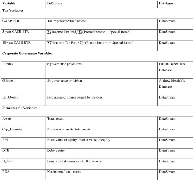
Table 1. Variables definitions and databases ... 11

Table 2. Panel A – Model 1 variables univariate analysis ... 14

Panel B – Model 1 variables correlation matrix ... 14

Table 5. Model 1 regressions ... 21

Table 8. Model 4 regressions for “excessive tax payers” ... 28

Table 11. Model 4 regressions for “tax savers” ... 31

Table 12. Model 5 regressions for “tax savers” ... 32

(7)

Corporate Governance and Taxes

1

1. Introduction

The conflicts between shareholders and managers have been documented for a long time. Jensen and Meckling (1976) suggest that if managers try to maximize their utility, they will not always act in the best interests of the shareholders. Thus, on firms where shareholders actions are constrained, managers can act contrarily to the will of the shareholders and, more importantly, can manage the company for their own purposes, instead of managing it in order to maximize the companies’ value and the shareholders’ wealth. On the other extreme, on firms where management has few powers, shareholders have higher control and can easily replace directors. However, shareholders powers decreased significantly after the 1980s. Many firms created takeover defenses and managers’ protection clauses in response to a series of hostile takeovers in that decade. These clauses, which Gompers et al. (2003) define as “governance provisions”, increase managers’ security and decrease shareholders powers.

These conflicts between managers and shareholders and its fiscal implications have been studied in recent literature. However, most of these studies only analyze the impact that Corporate Governance characteristics have on current year’s tax related variables. For instance, Minnick and Noga (2010) show that staggered boards are associated with higher tax rates, because stronger managers have fewer concerns with taxes. This means that if shareholders have more influence on a firm’s board, current year’s tax rates tend to be lower. Thus, it suggests that strong shareholders rights decrease current year’s effective tax rates.

In our paper there are two key sets of variables: Corporate Governance variables and tax variables. Corporate Governance variables are mostly based on the governance provisions described above. Gompers et al. (2003) and Bebchuk et al. (2004) create their Corporate Governance indexes that quantify the shareholders/ managers power. Thus, to capture the effect that Corporate Governance has on taxes, we use the Governance Index (G-Index, from now on; Gompers et al., 2003) and the Entrenchment Index (E-Index, from now on; Bebchuk et al., 2004). Additionally, we use Insider Ownership as a measure of Corporate Governance. In order to measure effective tax

(8)

2

rates we use two measures proposed by Dyreng et al. (2008): GAAP ETR and multi-year CASH ETR.

Our paper develops two different methodologies. In the first place, our paper follows the approach of Minnick and Noga (2010) and analyzes the relationship between Corporate Governance and current years’ tax rates. Similarly to them, we use GAAP and 5-year CASH ETR’s as tax variables. However, Dyreng et al. (2008) argue that it is relevant to study firms’ ability to manage taxes over periods as long as ten years. Therefore, we additionally use 10-year CASH ETR, in order to capture the effects of Corporate Governance characteristics on effective tax rates for a longer period. Unlike Minnick and Noga’s study, ours won’t include governance variables that they consider, namely “Number of board members”, “The percentage of directors who are independent”, “Age of the CEO” and “Staggered Boards”, using instead G-Index, E-Index and Insider Ownership. We expect that our results support the finding of Minnick and Noga (2010), by showing that stronger shareholders rights tend to reduce current years’ tax rates.

In the second place, we argue that current year’s tax rates should be considered when analyzing the connection between Corporate Governance and next years’ taxes. We consider that stronger shareholders rights have different impacts on future taxes, depending on whether firms have high or low tax rates. Thus, our paper not only analyzes the relationship between Corporate Governance and current year’s tax rates, but also studies the reaction that firms with strong or weak shareholders rights have after a year of excessive or low tax rates. We develop a unique approach – as far as we know - to the link between Corporate Governance and taxes. We create two groups based on their effective tax rate. On one hand, we consider firms that have excessive tax rates in a given year which we called “excessive tax payers”; on the other hand, we take into account firms that have low tax rates in a given year (“tax savers”). For each firm that is an “excessive tax payer” or a “tax saver” we studied the effective tax rates in the following three years. This approach expands previous literature on the relationship between Corporate Governance and taxes in two ways. On one hand, we not only analyze the effects of Corporate Governance on taxes for an unrestricted sample, but also for two firms’ groups, which may reveal some group-specific effects. On the other

(9)

3

hand, we develop a dynamic analysis, by studying tax rates for the three years that follow an excessive or a low tax rate report. We expect that within the “excessive tax payers”, the firms with stronger shareholders rights have lower tax rates, comparatively to those with weaker shareholders rights, during the years that follow an excessive tax rate’s year. However, we consider that stronger shareholders have fewer concerns with next years’ taxes when current tax rates are low. Therefore, we expect no significant relationship between Corporate Governance and tax rates for the firms within the “tax savers” group.

Our results show that, for the whole sample, stronger shareholders rights are associated with lower effective tax rates, which is consistent with the findings of Minnick and Noga (2010). Additionally, they suggest that, within the firms that paid excessive tax rates in a given year, firms with stronger shareholders rights have lower effective tax rates, relatively to firms with weaker shareholders rights, during the next 2 years. However, within the firms that paid low taxes in a given year, there is no evidence that suggests that Corporate Governance characteristics influence effective tax rates in the following years. These results suggest that current year’s tax rates must be taken into account when analyzing the connection between Corporate Governance and taxes, since Corporate Governance has a significant fiscal impact on next year´s tax rates for firms with high current tax rates but not on firms with low current tax rates.

The remainder of this paper is organized as follows. Section 2 resumes previous literature on the relation between Corporate Governance and tax management activities and develops the paper’s hypothesis. Section 3 describes the variables and selects the sample. Section 4 explains the estimation procedure and shows the results of hypothesis 1. Section 5 presents the results of hypotheses 2 and 3. The final section is a brief summary of the paper.

(10)

4

2. Literature Review and Hypotheses Development

2.1. Literature Review

There has been a large set of studies analyzing the various effects that Corporate Governance has on a firm. The majority of these studies try to measure the effect that strong shareholder rights has on firm’s performance and value (Chang and Zhang, 2010; Bhagat and Bolton, 2008; Brown and Caylor, 2006). Most of those studies conclude that stronger shareholder rights have a positive effect on both, although some others don’t find a significant relation between Corporate Governance and firm performance (Fodor and Diavastapoulos, 2010).

However, previous literature on the nexus between Corporate Governance and tax rates is not as wide. Minnick and Noga’s study (2010) is the closest to ours and is one of the firsts – as far as we know - to analyze the relationship between Corporate Governance and taxes using CASH ETR as a tax measure. Their results show that staggered boards are associated with higher GAAP and 5-year CASH ETR’s. This means that stronger shareholder rights, particularly the ability to replace the boards, result in lower current year’s effective tax rates. However, other Corporate Governance variables, such as board size, independence and age of the CEO, are not strongly related with effective tax rates.

Some studies lead to similar conclusions, despite not using the same methodology. Huang et al. (2010) find that firms with stronger shareholder rights have less income-increasing discretionary accruals. They conclude that stronger shareholder rights discourage managers from reporting excessive earnings; despite the fact that this study doesn’t directly analyze the impact of Corporate Governance variables on effective tax rates, we assume that shareholders discourage excessive earnings in order to reduce their firms’ tax burden. Thus, stronger shareholder rights also should prevent excessive effective tax rates.

Despite the fact that there are few studies that study the connection between Corporate Governance and effective tax rates, there is a larger set of studies studying

(11)

5

the fiscal consequences of Corporate Governance characteristics. Nevertheless, many of those studies have been leading to ambiguous results. For instance, there is no consensus on the connection between Corporate Governance and the quality of financial reports. Baber et al. (2009) find that firms accounting misstatements are less common in firms with stronger shareholders powers. On the other hand, Carcello et al., (2006) find that entrenched managers help improving the quality of financial reports, which means that stronger management powers lead to better financial reports. The same thing can be said about the link between Corporate Governance and earnings management. Chtourou et al. (2001) finds that larger boards with more experience and independent audit committees are associated with decreasing earnings management. Chen and Zhao (2008) show that staggered boards have fewer incentives to manage earnings.

On another study, Klein (2002) focuses on the link between Corporate Governance and tax management. She shows that there is a significant negative relation between audit committee independence and tax management, which means that if an audit committee is independent there is a smaller probability that the firm will manage taxes. She also finds that, in the one hand, a CEO sitting on the board’s compensation committee increases tax management and, in the other hand, a large outside shareholder sitting on the board’s audit committee decreases tax management.

Some other studies try to study the incentives of tax avoidance for firms with stronger and weaker governance. Desai and Dharmapala (2009) find that firms with high levels of institutional ownership have higher incentives to incur in tax management activities. In another study (Desai and Dharmapala, 2004), they show that managers’ incentive compensation tend to reduce book-tax differences, and thereby, reduce tax avoidance. Desai, along with other authors (Desai et al. 2004), also studied the best fiscal policies for countries with stronger/ weaker governance firms. Their study shows that if a country’s firms have weaker governance, an increase in the tax rate can reduce tax revenues, via tax management. Then, if their companies have better Corporate Governance, countries have higher incentives to raise taxes, because these firms are less likely to incur in tax management activities.

(12)

6

2.2. Hypotheses Development

As described above, previous literature on Corporate Governance and taxes focus on the current tax variables. Our first hypothesis also tries to test the effect that stronger or weaker shareholders rights have on current year’s tax rates. So we try to find evidence that supports the findings of Minnick and Noga (2010). Thus, we expect that stronger shareholders rights result in lower tax rates. So H1 is defined as:

H1: Stronger shareholders rights decrease effective tax rates.

For the development of our second and third hypotheses, we create two groups based on their effective tax rate. We define “excessive tax payers” as the firms that have excessive tax rates in a given year and “tax savers” as those who have low tax rates in a given year. Hypothesis 2 is centered on the “excessive tax payers” group and hypothesis 3 on the “tax savers” group. Similarly to H1, we expect that, within the “excessive tax payers” group, the firms with stronger shareholders rights are those with the lowest effective tax rates during the years that follow an excessive tax rate report. Huang et al. (2010) argue that stronger shareholders rights avoid excessive earnings. We consider that by doing so, shareholders aim to reduce firm’s tax burden. Thus, stronger shareholders powers should avoid excessive tax rates. This means that following a year of excessive tax rates, firms with stronger shareholders rights should have lower tax rates than firms with weaker shareholder rights. So, H2 can be defined as:

H2: Within the firms that have excessive tax rates in a given year, those with stronger shareholders rights have lower effective tax rates, comparatively to those with weaker shareholders rights, during the next k years (where k = 1,2,3).

Our third hypothesis analyzes the “tax savers” group. As said before, we try to demonstrate that current year’s tax rates is a factor that must be taken into account when analyzing Corporate Governance and tax rates. Therefore, we expect that stronger shareholders rights have different impacts on next years’ tax rates, depending on whether firms have a current excessive tax rate or a current low tax rate. We argue that shareholders have more concerns when tax rates are high but not so much when they are

(13)

7

low. Thus, we expect that stronger shareholders rights on firms with current year’s low tax rates have no significant impact on next years’ tax rates. So H3 can be defined as:

H3: Within the firms that have low tax rates in a given year, stronger shareholders rights have no significant impact on next k years’ effective tax rates, years (where k =1,2,3).

3. Variables Description and Sample Selection

3.1. Variables Description

As described above, our hypotheses test the impact that Corporate Governance has on effective tax rates (on the whole sample for hypothesis 1 and for two subsamples for hypotheses 2 and 3). This subsection describes and explains tax variables, Corporate Governance measures and firm-specific variables that are used in this paper’s models.

Tax variables

To measure effective tax rates we use GAAP ETR and 5-year and 10-year CASH ETR’s (Dyreng et al. (2008)). GAAP ETR is an annual rate defined as:

However, this one-year measure is not the best to the purpose of this study. There may occur some significant yearly variations that are not seized by GAAP ETR. Also, by using Tax Expense in the numerator, it does not take into account deferred tax expense (3.A)

(14)

8

(3.B) and refunds from the IRS. To solve those problems, Dyreng et al. (2008), propose a multi-year rate (5 or 10 years, in this study) defined as:

For instance, if we want to calculate the CASH ETR value of a firm in 1990, we sum the cash taxes paid and the pretax incomes less special items during the period 1981-1990 (for a 10 year rate) or during the period 1986-1990 (for a 5 year rate). On the one hand, this will decrease the effects of years with unusually large or small effective tax rates, relatively to the GAAP ETR and, on the other, will take into account deferred tax expenses. Comparatively to other studies, this will be one of the firsts (to our knowledge) to use 10-year CASH ETR as an effective tax rate. We add this variable because Dyreng et al. (2008) argue that it is pertinent to test the ability that firms have in avoiding taxes over periods as long as ten years.

Corporate Governance variables

In order to measure Corporate Governance characteristics, we use two Corporate Governance indexes and Insider Ownership. By considering Insider Ownership individually, there could be revealed some effects associated to that variable. Also, the use of two indexes may reveal that effective tax rates are impacted by some Corporate Governance provisions, but not by all of them.

The first Corporate Governance measure is the Governance Index (G-Index; Gompers et al. (2003)). This index considers 24 governance provisions1 that reduce shareholders powers. A firm’s score ranges from 0 to 24 and high scores reflect high

(15)

9

management power or weak shareholders rights; on the contrary low scores are a sign of low management power or strong shareholders rights (Gompers et al., 2003).

The second measure is the Entrenchment Index (E-Index; Bebchuk et al. (2004)). Their authors argue that E-Index is more refined index than G-Index, because it only takes into account the 6 most important governance provisions2, instead of the original G-Index’s 24. A firm’s score ranges from 0 to 6 and similarly to the G-Index a high (low) score is associated with weak (strong) shareholders rights and high (weak) management power.

Both indexes apply their scores to 1500 companies from the Standard & Poor’s 500 as well as from the annual lists of the largest corporations in the publications of

Fortune, Forbes, and Businessweek.

Additionally, we use Insider Ownership (Ins_Owner) as a Corporate Governance measure. Previous research has shown that a higher percentage of outside directors has a positive impact on stock returns (Byrd and Hickman, 1992; Weisbach, 1988). We argue that the percentage of shares owned by insiders could also impact effective tax rates. This variable is defined, by DataStream, as the percentage of shares owned by officers, directors and their immediate families, shares held in trust, shares of the company held by any other corporation, shares held by pension/benefit plans and shares held by individuals who hold more than 5% or more of the outstanding shares.

Firm-specific Variables

In this study, we use a set of variables to measure firm characteristics that may affect effective tax rates. By using them, we control for firm-specific characteristics, like size, growth, capital intensity, debt and profitability.

As Dyreng et al. (2008) suggested, firms’ size and growth influence effective tax rates. Thus, following Minnick and Noga (2010), we use the variable assets in its

(16)

10

logarithmic form (Log_Assets) to control the firms’ size and the ratio between the book value of equity and its market value (BM) as a proxy of firms’ growth

Secondly, we consider the effects of amortizations and depreciations on effective tax rates. So, we use the ratio between non-current assets and total assets (Cap_Intensity) to measure companies’ capital intensity.

Many authors (Minnick and Noga, 2010; Huang et al., 2010; Noor et al., 2010; Baber et al., 2009) highlight the importance of debt tax shields and the importance of controlling for that. In order to do so, we use the ratio debt-to-equity (DTE).

Minnick and Noga (2010) argue that firms with negative earnings should be controlled, because their inclusion on the regression may lead to biased analysis and results. To control for these firms, we use a dummy variable (D_Earn) that is equal to one if earnings are positive and zero otherwise.

Additionally, we use the variable Return on Assets (ROA) as a measure of firms’ profitability (accordingly to Noor et al., 2010).

3.2. Sample Selection

G-Index and E-Index’s scores were collected from Yale School of Management and on Harvard Law School’s online databases, respectively. Both indexes’ scores are available only for the years of 1990, 1993, 1995, 1998, 2000, 2002, 2004 and 2006 and cover 1500 companies from the Standard & Poor’s 500 as well as from the annual lists of the largest corporations in the publications of Fortune, Forbes, and Businessweek. We follow the data treatment proposed by Huang et al. (2010), in order to expand the years analyzed. They had discussions with the author of the IRRC publications and found that a firm’s E-Index’s score applies to more than just one year. In fact, a firm’s score in one year can be applied to the subsequent or previous years in most cases. With that in mind, we analyzed the scores for the G-Index and for the E-Index and found that they were very regular during those years, for the large majority of the firms. So we assume that the G-Index and E-Index’ scores for the fiscal year of 1990, can be applied

(17)

11

to 1991 and 1992; the scores of 1993 to 1994; the scores of 1995 to 1996 and 1997; the scores of 1998 to 1999; the scores of 2000 to 2001; the scores of 2002 to 2003; the scores of 2004 to 2005; and the scores of 2006 to 2007.

The construction of tax variables required a collection of DataStream’s data from 1983 to 2007 in order to be able to calculate multi-year CASH ETR’s. All the other variables, including Insider Ownership and firm-specific variables, were extracted from DataStream’s database from 1990 to 2007. Table 1 resumes the variables, their construction and their sources.

Table 1 – Variables definitions and databases

Variable Definition Database

Tax Variables

GAAP ETR Tax expense/pretax income DataStream

5-year CASH ETR DataStream 10-year CASH ETR DataStream

Corporate Governance Variables

E Index 6 governance provisions Lucian Bebchuk’s

Database

G Index 24 governance provisions Andrew Metrick’s

Database Ins_Owner Percentage of shares owned by insiders DataStream

Firm-specific Variables

Assets Total assets DataStream

Cap_Intensity Non-current assets/ total assets DataStream BM Book value of equity/ market value of equity DataStream

DTE Debt/ equity DataStream

D_Earn Equals to 1 if earnings > 0; 0 otherwise DataStream

(18)

12

4. Hypothesis 1 development

4.1. Methodology and Univariate Analysis

In this subsection we explain the methodology used to test hypothesis 1. As described above, hypothesis 1 suggests that stronger shareholders rights decrease effective tax rates.

In order to measure the effect of corporate governance variables on taxes we use three different approaches. Nevertheless, the methodology used on the three models is similar. We use OLS estimations with year and SIC-code industry fixed effects for all three of them3, with outliers’ exclusion (1%) for all the variables in order to create more centric estimations. Furthermore, we only consider positive (but not bigger than 100%) values for the effective tax rates, because many of the negative results were due to negative income and not tax refunding. So, considering them might bias our analysis. The explanatory variables are the same for the three models and the only difference between the models relies on the dependent variable.

Model 1

On the first model we use the tax variable GAAP ETR and on the second and on the third models we use CASH ETR for 5 and 10 years, respectively. Each model has three equations, depending if the corporate governance variable is the E-Index, the G-Index or Insider Ownership. For all three models we use the firms-specific variables described above to control for size, growth, debt, capital intensity and profitability. Thus, the first model’s equations are the followings:

3_{The Hausman test rejected the hypothesis of random effects’ estimators being efficient and confirmed}

the hypothesis of fixed effects’ estimators being consistent, for both SIC-code industry code and year effects.

(19)

13 (4.A) (4.B) (4.C)

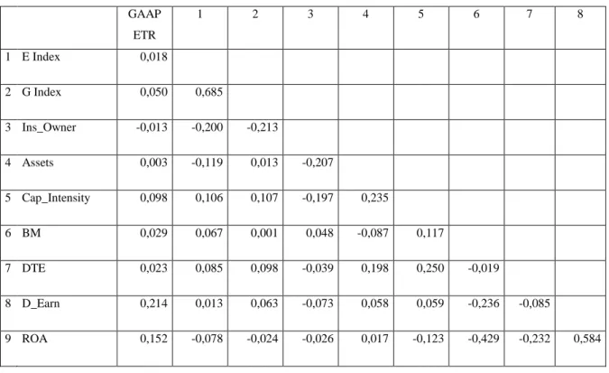
This analysis covers the years from 1990 to 2007 and with the data treatment described above the sample is restricted to 9211 year-firm observations. Panel A of Table 2 shows the univariate analysis for all the variables and Panel B shows the Pearson’s correlations’ matrix.

As panel A shows, most of the firms have strong shareholders rights. Both E-Index (its mean and median are, respectively, 2.431 and 3) and G-E-Index (9.4 and 9 respectively) have small values (E-Index ranges from 0 to 6 G-Index from 0 to 24). Although some firms were able to get the maximum E-Index score, the highest G-Index score for this sample (18) was far from the maximum G-Index value (24). We can also conclude that the sample is majorly constituted by large firms with strong capital intensity (most firms have more than 50% of non-current assets). Also, many of the firms of this sample have a market value much higher than its book value (most of the firms have a market value that is the double of the book value). We can also deduce that 92.4% of the firms have positive earnings.

Panel B shows that there is no indication of linear correlation between the explanatory variables. As expected, and because the E-Index is based on a sub-set of the original G-Index provisions, these variables have a strong positive correlation (0.685). All the other variables are weakly correlated, with the exception of D_Earn and ROA (0.584).

(20)

14

Table 2 – Panel A – Model 1 variables’ univariate analysis

Variable Mean Standard

Deviation

Minimum Median Maximum

GAAP ETR 0,339 0,109 0,000 0,356 0,999 E Index 2,431 1,283 0,000 3,000 6,000 G Index 9,400 2,696 2,000 9,000 18,000 Ins_Owner 14,199 15,311 0,040 10,700 81,480 Assets 5.058.907 9.541.312 48.916 1.547.900 106.159.000 Cap_Intensity 0,556 0,218 0,056 0,560 0,953 BM 0,462 0,293 0,008 0,408 2,253 DTE 1,579 1,639 0,009 1,177 18,363 D_Earn 0,924 0,266 0,000 1,000 1,000 ROA 0,060 0,070 -0,537 0,057 0,307

Table 2 – Panel B – Model 1 variables’ correlation matrix

GAAP ETR 1 2 3 4 5 6 7 8 1 E Index 0,018 2 G Index 0,050 0,685 3 Ins_Owner -0,013 -0,200 -0,213 4 Assets 0,003 -0,119 0,013 -0,207 5 Cap_Intensity 0,098 0,106 0,107 -0,197 0,235 6 BM 0,029 0,067 0,001 0,048 -0,087 0,117 7 DTE 0,023 0,085 0,098 -0,039 0,198 0,250 -0,019 8 D_Earn 0,214 0,013 0,063 -0,073 0,058 0,059 -0,236 -0,085 9 ROA 0,152 -0,078 -0,024 -0,026 0,017 -0,123 -0,429 -0,232 0,584

(21)

15

(4.D)

(4.E)

(4.F) Model 2

On the second model we use CASH ETR for 5 years as the dependent variable. Similarly to the first model, we have three equations, depending whether the corporate governance variable is the E-Index, the G-Index or Insider Ownership. So the equations are the followings:

The results of this model should be a lot more conclusive than the results of the first model. Even though the sample is considerably smaller, because every observation requires data from 5 years in a row, the estimations should be a lot more significant: this 5-year range may capture some long-term tax management activities.

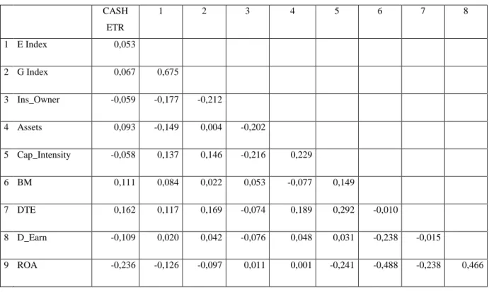
This analysis covers the years from 1991 to 2007. It should be noted that, for example, the values of CASH ETR for the year 1991 comprehend tax data between 1987 and 1991 (hence the 5-year range of this measure). The sample is restricted to 4887 year-firm observations. Panel A of Table 3 shows the univariate analysis for all the variables and Panel B shows the Pearson’s correlations’ matrix.

(22)

16

Table 3 –Panel A – Model 2 variables’ univariate analysis

Deviation

CASH ETR 0,176 0,158 0,000 0,131 0,995 E Index 2,397 1,297 0,000 2,000 6,000 G Index 9,491 2,738 2,000 9,000 18,000 Ins_Owner 13,413 14,831 0,040 9,560 82,340 Assets 6.293.738 12.355.912 91.079 1.839.100 135.695.000 Cap_Intensity 0,553 0,212 0,043 0,560 0,952 BM 0,416 0,281 0,018 0,357 4,954 DTE 1,413 1,343 0,004 1,076 15,272 D_Earn 0,950 0,219 0,000 1,000 1,000 ROA 0,074 0,059 -0,224 0,069 0,320

Table 3 – Panel B - Model 2 variables’ correlation matrix

CASH ETR 1 2 3 4 5 6 7 8 1 E Index 0,053 2 G Index 0,067 0,675 3 Ins_Owner -0,059 -0,177 -0,212 4 Assets 0,093 -0,149 0,004 -0,202 5 Cap_Intensity -0,058 0,137 0,146 -0,216 0,229 6 BM 0,111 0,084 0,022 0,053 -0,077 0,149 7 DTE 0,162 0,117 0,169 -0,074 0,189 0,292 -0,010 8 D_Earn -0,109 0,020 0,042 -0,076 0,048 0,031 -0,238 -0,015 9 ROA -0,236 -0,126 -0,097 0,011 0,001 -0,241 -0,488 -0,238 0,466

(23)

17

(4.G)

(4.H) The conclusions from the variables’ univariate analysis are similar to the first model. After all, this subset of firms is a sub-sample of the first model’s sample. As panel A shows, most of the firms have low E-Index and G-Index scores which reiterates the idea that most of the firms of the sample have strong shareholders rights. Comparing the statistical scores for GAAP ETR (table 1, panel A) and CASH ETR (table 2, panel B), we can see that there is an enormous difference in the values. This shows that firms’ 5-year CASH ETR is much smaller than GAAP ETR (the mean and the median of each are, respectively, 0.176 vs. 0.339 and 0.131 vs. 0.356) which is consistent with the findings of Minnick and Noga, 2010).

There is still no evidence of linear correlation problems, notwithstanding that ROA has some high correlation values (-0,488 with BM and 0,466 with D_Earn). Unlike the model 1, three firm-specific variables have negative correlations with CASH ETR, while in the first model none of the variables was negatively correlated with GAAP ETR.

Model 3

On the third model we use CASH ETR for 10 years as the dependent variable. This is an unused measure of effective tax rates on previous literature on the nexus between Corporate Governance and taxes, but we expect similar results to 5-year CASH ETR. We have three equations, depending whether the corporate governance variable is the E-Index, G-Index or Insider Ownership. So the equations are the followings:

(24)

18

(4.I)

The sample is even smaller than the one on model 2, because now every observation requires data from 10 years in a row. Similarly to the model 2, this 10-year range may capture some long-term tax management activities.

This analysis will cover the years from 1992 to 2007. It should be noted that, for example, the values of CASH ETR for the year 1992 comprehend tax activity between 1983 and 1992 (hence the 10-year range of this measure). The sample is restricted to 2582 year-firm observations. Panel A of Table 4 shows the univariate analysis for all the variables and Panel B shows the Pearson’s correlations’ matrix.

All the statistical scores are very similar to the second model, so the univariate analysis is identical. Equally to 5-year CASH ETR, 10-year CASH ETR is much smaller than GAAP ETR (the means are, respectively, 0.187 and 0.339 and the medians are 0.143 and 0.356).

(25)

19

Table 4 –Panel A – Model 3 variables univariate analysis

Deviation

CASH ETR 0,187 0,155 0,000 0,143 0,990 E Index 2,443 1,290 0,000 3,000 5,000 G Index 9,641 2,653 2,000 10,000 18,000 Ins_Owner 12,734 14,335 0,040 8,945 82,580 Assets 8.506.920 16.859.910 107.435 2.390.591 164.719.000 Cap_Intensity 0,558 0,201 0,047 0,572 0,953 BM 0,409 0,260 0,023 0,352 1,890 DTE 1,490 1,528 0,029 1,095 17,750 D_Earn 0,945 0,227 0,000 1,000 1,000 ROA 0,073 0,058 -0,186 0,068 0,317

Table 4 – Panel B - Model 3 variables’ correlation matrix

CASH ETR 1 2 3 4 5 6 7 8 1 E Index 0,038 2 G Index 0,039 0,627 3 Ins_Owner -0,069 -0,168 -0,195 4 Assets 0,079 -0,220 -0,052 -0,194 5 Cap_Intensity -0,071 0,157 0,142 -0,234 0,206 6 BM 0,048 0,158 0,046 0,069 -0,128 0,167 7 DTE 0,149 0,098 0,162 -0,070 0,120 0,296 -0,085 8 D_Earn -0,095 0,013 0,026 -0,063 0,064 0,025 -0,253 -0,012 9 ROA -0,173 -0,135 -0,089 0,028 0,055 -0,257 -0,533 -0,205 0,477

(26)

20

4.2. Multivariate Analysis

This subsection analyzes the results of the models described above. The results for models 1, 2 and 3 are shown on tables 5, 6 and 7 respectively.

As the tables demonstrate, there is a positive relationship between the Corporate Governance indexes’ scores and effective tax rates. In fact, tables 5 and 6 shows that the coefficients associated with the Corporate Governance indexes show a significant positive relation with GAAP ETR and 5-year CASH ETR. Table 7 is not as elucidative: the coefficient associated with E-Index has the expected sign but is not significant; furthermore, G-Index appears to have a negative relationship with 10-year CASH ETR (although it is not significant either). On the other hand, all the tables show that there is no significant relationship between Insider Ownership and effective tax rates.

As for the firm-specific variables, the results suggest that higher tax rates are associated with bigger firms (consistent with Rego, 2003) and with firms who have higher growth potential (consistent with Dyreng et al., 2008), particularly on tables 6 and 7. However, other variables’ coefficients aren’t as conclusive: table 5 points to different conclusions than tables 6 and 7. For instance, tables 6 and 7 suggest that firms with higher capital intensity tend to have lower tax rates, which could reflect the effect of higher depreciations and amortizations; yet, the results on table 5 point to the contrary.

Although the lack of significance with 10-year CASH ETR, globally the results seem to indicate that there is a positive relationship between Corporate Governance indexes and effective tax rates, both on GAAP ETR and on 5-year CASH ETR’s estimations. Given that high (low) scores on the indexes imply weakest (strongest) shareholders powers, the results mean that stronger shareholders powers lead to lower effective tax rates. These results are consistent with H1 and with the findings of Huang et al. (2010) and Minnick and Noga (2010).

(27)

21

Table 5 – Model 1 regressions. On regression 1 the Corporate Governance variable considered was E-Index.

Regression 2 uses G-Index as the Corporate Governance variable. Regression 3 uses Insider Ownership as the Corporate Governance variable. For all the regressions there were used year and SIC code industry controls. All variables’ outliers were excluded at the 1% level. For all the regressions it was used the OLS estimation method. * means 10% individual significance of the corresponding variable, ** means 5% individual significance of the corresponding variable and *** means 1% individual significance of the corresponding variable. In parenthesis are the observed t-statistic values.

Dependent Variable: GAAP ETR

1 2 3 C 0,222512*** 0,22111*** 0,227958*** (4,734845) (4,705547) (4,80445) E_INDEX 0,002053** (2,353249) G_INDEX 0,001255*** (3,012399) INS_OWNWERSHIP -0,000064 (-0,815603) LOG(ASSETS) -0,000196 -0,000602 -0,000533 (-0,221221) (-0,676248) (-0,578742) CAP_INTENSITY 0,052341*** 0,052368*** 0,053854*** (6,891512) (6,909339) (7,117818) BM 0,030556*** 0,030741*** 0030990*** (6,794225) (6,838956) (6,885291) DTE 0,001637** 0,001655** 0,001789** (2,174368) (2,200778) (2,368225) D_EARN 0,058409*** 0,058041*** 0,058992*** (11,50703) (11,42820) (8,150903) ROA 0,175626*** 0,176030*** 0,173063*** (8,264047) (8,286382) (8,150903) R2 0,150972 0,151301 0,150519 Adjusted R2 0,143158 0,143489 0,1427 Sample Size 9211 9211 9211

(28)

22

Table 6 - Model 2 regressions. On regression 1 the Corporate Governance variable considered was E-Index.

Regression 2 uses G-Index as the Corporate Governance variable. Regression 3 uses Insider Ownership as the Corporate Governance variable. For all the regressions there were used year and SIC code industry controls. All variables’ outliers were excluded at the 1% level. For all the regressions it was used the OLS estimation method. * means 10% individual significance of the corresponding variable, ** means 5% individual significance of the corresponding variable and *** means 1% individual significance of the corresponding variable. In parenthesis are the observed t-statistic values.

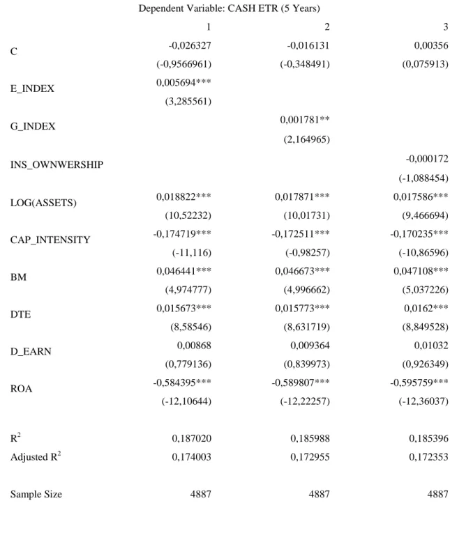
Dependent Variable: CASH ETR (5 Years)

1 2 3 C -0,026327 -0,016131 0,00356 (-0,9566961) (-0,348491) (0,075913) E_INDEX 0,005694*** (3,285561) G_INDEX 0,001781** (2,164965) INS_OWNWERSHIP -0,000172 (-1,088454) LOG(ASSETS) 0,018822*** 0,017871*** 0,017586*** (10,52232) (10,01731) (9,466694) CAP_INTENSITY -0,174719*** -0,172511*** -0,170235*** (-11,116) (-0,98257) (-10,86596) BM 0,046441*** 0,046673*** 0,047108*** (4,974777) (4,996662) (5,037226) DTE 0,015673*** 0,015773*** 0,0162*** (8,58546) (8,631719) (8,849528) D_EARN 0,00868 0,009364 0,01032 (0,779136) (0,839973) (0,926349) ROA -0,584395*** -0,589807*** -0,595759*** (-12,10644) (-12,22257) (-12,36037) R2 0,187020 0,185988 0,185396 Adjusted R2 0,174003 0,172955 0,172353 Sample Size 4887 4887 4887

(29)

23

Table 7 - Model 3 regressions. On regression 1 the Corporate Governance variable considered was E-Index.

Regression 2 uses G-Index as the Corporate Governance variable. Regression 3 uses Insider Ownership as the Corporate Governance variable. For all the regressions there were used year and industry controls. All variables’ outliers were excluded at the 1% level. For all the regressions it was used the OLS estimation method. * means 10% individual significance of the corresponding variable, ** means 5% individual significance of the corresponding variable and *** means 1% individual significance of the corresponding variable. In parenthesis are the observed t-statistic values.

Dependent Variable: CASH ETR (10 Years)

1 2 3 C -0,039396 -0,023409 -0,026958 (-0,52967) (-0,31557) (-0,359981) E_INDEX 0,002639 (1,080358) G_INDEX -0,001233 (-1,065151) INS_OWNWERSHIP -0,000062 (-0,275841) LOG(ASSETS) 0,018076*** 0,017784*** 0,017451*** (7,718546) (7,691783) (7,207553) CAP_INTENSITY -0,182592*** -0,17743*** -0,17974*** (-8,213649) (-8,021623) (-8,144222) BM 0,051668*** 0,053406*** 0,052914*** (3,469848) (3,590116) (4,554549) DTE 0,018916*** 0,01927*** 0,019121*** (8,431775) (8,574434) (8,503693) D_EARN -0,001765 -0,000277 -0,001107 (-0,12071) (-0,018957) (-0,075737) ROA -0,455937*** -0,459214*** -0,457745*** (-6,523102) (-6,572801) (-6,547807) R2 0,201496 0,201486 0,201149 Adjusted R2 0,178254 0,178243 0,177897 Sample Size 2582 2582 2582

(30)

24

5. Hypotheses 2 and 3: “Excessive tax payers” vs. “tax savers”

Although the results for the whole sample indicate that strong shareholders rights reduce companies’ tax burden, this trend may not be verified for all firms. We particularly emphasize two groups: “excessive tax payers” and “tax savers”. Previous literature on Corporate Governance and taxes focus on the effects that stronger shareholders rights have on a tax related variable, for a sample that indiscriminately contains firms with low, medium and high tax rates. In this section, we focus on firms that have high or low tax rates in a given year, and analyze the impact that Corporate Governance has on next three years’ tax rates. By doing so, we try to demonstrate that current year’s tax rates must be taken into account when analyzing Corporate Governance and tax rates. Thereby, we expect that stronger shareholders rights have different impacts on next years’ tax rates, depending on whether firms have a current excessive tax rate or a current low tax rate.

The “excessive tax payers” group contains firms that have effective tax rates (either GAAP or multi-year CASH ETR’s) higher than 40% and the “tax savers” group contains all the firms that have effective tax rates lower than 10% on a given year. Then, for each year that a firm had excessive or low tax rates we analyze the effective tax rates for the following three years. If an “excessive tax payer” has strong shareholders rights, it is expected, according to H2, that the effective tax rates will be smaller than on firms with weak shareholders rights, in the next years. According to H3, we can’t say the same thing about the “tax savers” group, because we consider that stronger shareholders have fewer concerns with next years’ taxes when current year’s tax rates are low.

This constitutes a new approach to the link between Corporate Governance and taxes, so there is no evidence on literature that support the definition of the reference tax rates of 40% for “excessive tax payers” and 10% for “tax savers”.

However, we consider that those values are appropriate. On the first place, the maximum federal marginal tax rate in the United States is 35%4, so 40% seems like an

(31)

25

appropriate value to distinguish between excessive and non-excessive tax payers. Besides, the mean of the highest deciles of the distributions of GAAP and 5-year and 10-year CASH ETR’s is very close to 40% (38.98%).

10% also seems like an appropriate value to distinguish between tax savers and non-savers because the minimum federal marginal tax rate in the United States is 15%5. The mean of the lowest deciles of the distributions of GAAP and 5-year and 10-year CASH ETR’s is very close to 10% (10.05%). Furthermore, we believe that the conclusions for those reference tax rates may be extensible to another tax rates.

Similarly to the models of Hypothesis 1, we construct 3 additional models, depending on the dependent variable. However, in all the following models we don’t use the variable Insider Ownership as a measure of Corporate Governance, due to its lack of significance revealed on previous estimations. Similarly to the H1 procedure, we use OLS estimations with year and SIC-code industry fixed effects for all three models6, with outliers’ exclusion (1%) for all the variables in order to create more centric estimations. Also, we only consider positive (but not bigger than 100%) values for the effective tax rates, because many of the negative results were due to negative income and not tax refunding and considering them could bias our analysis.

Model 4 uses GAAP ETR as dependent variable. However, because we try to verify the effect of Corporate Governance on effective tax rates in 3 years following an excessive/ low tax rate, in this model we use GAAP ETR for the year t+k (where k=1,2,3). Similarly, all control variables values considered are related to the year t+k. However both E and G Indexes scores are for the year t. We use this methodology, because we want to test if a firm that has excessive or low tax rates and strong shareholder rights, in this moment, will decrease his tax burden in the next three years. Thus, the variable that represents Corporate Governance must reflect current year situation.

5_{For the year of 2012}

6_{The Hausman test rejected the hypothesis of random effects’ estimators being efficient and confirmed}

(32)

26 (5.A) (5.B) (5.C)

This model will be used both for “excessive tax payers” as for “tax savers”. Model 5 and 6 are similar to 4, with the only difference being the dependent variable.

This new approach has two important contributions to previous literature. In the first place, to our knowledge, we are the firsts to analyze not only the whole sample but also two firms’ groups. This methodology should isolate some effects that are specific to each group. Secondly, we develop a dynamic analysis, by studying the impact that stronger shareholders rights have on the effective tax rates on the years that follow an excessive or a low tax report.

Tables 8, 9 and 10 suggest that “excessive tax payers” with low governance indexes’ scores (particularly E-Index) significantly have lower effective tax rates, comparatively to those with high governance indexes’ scores, during the 2 years that follow a year of an excessive effective tax rate. However, G-Index lacks some significance, particularly on tables 7 and 9. This lack of significance may occur because E-Index is, according to their authors (Bebchuk et al., 2004), a more refined index in comparison with G-Index, by taking into account only the 6 most important governance

(33)

27

provisions, whereas G-Index contain some governance provisions that may bias the results and may lead to this lack of significance.

These results mean that within the firms that belong to the “excessive tax payers” group, those with stronger shareholders rights have lower taxes, relatively to those with weaker shareholders rights, during two years. This means that after a year of excessive tax rates, the firms with stronger shareholders rights are the ones with the lowest effective tax rates during the next 2 years, which is consistent with H2.

As for H3, as expected, Tables 11, 12 and 13 show that there is no significant relation between governance indexes’ scores and effective tax rates for any considered period. In fact, only table 13 (and only for G-Index) suggests that amongst the “tax savers” firms, those who have strong shareholders rights have the lowest effective tax rates during the years following a low tax rate report. This lack of significance could mean that Corporate Governance characteristics have a more significant role on firms with high tax rates than on firms with low tax rates. For firms with high tax rates in a given year, stronger shareholders rights have a significant impact. Amongst those firms, those with stronger shareholders rights have the lowest tax rates during the next two years. On the other hand, stronger shareholders rights don’t have a significant impact on tax burden for firms with low tax rates.

Overall, our results show that Corporate Governance plays a significant role for the firms that have excessive tax rates in a given year during the two next years. In fact, there is a significant difference between the behavior of firms with strong and weak shareholders rights, after a year of excessive tax rates. During the next two years, firms with stronger shareholders rights have lower taxes than firms with weaker shareholders rights, which suggest that stronger shareholders rights control excessive tax rates. However, there is no significant relationship between Corporate Governance and next years’ effective tax rates, after a year of low tax rates. This means that stronger shareholders rights have different impacts on next years’ tax rates, depending on whether firms have a current excessive tax rate or a current low tax rate, which supports our argument that current year’s tax rates must be taken into account when analyzing the connection between Corporate Governance and tax rates.

(34)

28

Table 8 – Model 4 regressions for “excessive tax payers”. For all the regressions there were used year and SIC

code industry controls. For all the regressions it was used the OLS estimation method. * means 10% individual significance of the corresponding variable, ** means 5% individual significance of the corresponding variable and *** means 1% individual significance of the corresponding variable. In parenthesis are the observed t-statistic values.

“EXCESSIVE TAX PAYERS” Dependent Variable: GAAP ETRt+k

1 year after 2 years after 3 years after

C -0,05336 -0,043463 -0,196242 -0,130952 -0,179773 -0,173374 (-0,32791) (-0,263129) (-1,102475) (-0,729979) (-0,93722) (-0,90089) E_INDEXt 0,020754*** 0,014651* -0,003863 (2,753193) (1,935156) (-0,485085) G_INDEXt 0,003471 -0,002106 -0,001962 (1,216336) (-0,687644) (-0,627057) LOG(ASSETS)t+k 0,016313 0,016347 0,025014** 0,024001* 0,0283** 0,028536** (1,394144) (1,390775) (2,001175) (1,916362) (2,140035) (2,160025) CAP_INTENSITYt+k 0,045142 0,056184 0,114658** 0,12091** 0,053935 0,053277 (0,742434) (0,922596) (2,047858) (2,153927) (0,889765) (0,881263) BMt+k 0,052392** 0,051522** 0,030091 0,030711 0,023415 0,022701 (2,397582) (2,344743) (1,433686) (1,456209) (1,009222) (0,977586) DTEt+k -0,001081 -0,000656 -0,006856** -0,00592* -0,001799 -0,001877 (-0,280847) (-0,170036) (-2,917233) (-1,746369) (-0,487276) (-0,50932) D_EARNt+k 0,115297*** 0,116898*** 0,121636*** 0,122512*** 0,135598*** 0,136384*** (6,685521) (6,751802) (7,504314) (7,538272) (7,774633) (7,787946) ROAt+k 0,05006 0,041322 -0,148591 -0,143518 -0,291065*** -0,293868*** (0,558762) (0,458994) (-1,633043) (-1,572827) (-2,746496) (-2,772721) R2 0,553839 0,550019 0,590155 0,588106 0,602234 0,602341 Adjusted R2 0,24071 0,234209 0,315672 0,312251 0,326702 0,326883 Sample Size 1211 1211 1093 1093 998 998

(35)

29

“EXCESSIVE TAX PAYERS” Dependent Variable: CASH ETRt+k (5 years)

C -0,790759 -1,216449* -0,106736 -1,475701 -1,407749 -3,170128*** (-1,22861) (-1,65907) (-0,109882) (-1,455778) (-1,389506) (-3,038585) E_INDEXt 0,062242** 0,115648*** 0,099247** (2,168508) (2,716869) (2,625504) G_INDEXt 0,015181 0,038939** 0,051244*** (0,995104) (2,19078) (3,398471) LOG(ASSETS)t+k 0,079898* 0,105995** 0,030741 0,112373* 0,102508 0,202289*** (1,664424) (2,211788) (0,474559) (1,755396) (1,541713) (3,120129) CAP_INTENSITYt+k -0,027096 0,048118 -0,057942 0,062229 0,029736 0,071413 (-0,132562) (0,236365) (-0,217229) (0,238413) (0,14285) (0,357966) BMt+k 0,151938** 0,149659** 0,149855** 0,134102* 0,168282** 0,162027** (2,455153) (2,350523) (2,011152) (1,784627) (2,514826) (2,476568) DTEt+k -0,030013* -0,026311 -0,040607* -0,047768** -0,023501 -0,040717*** (-1,798484) (-1,562715) (-1,974384) (-2,207876) (-1,606621) (-2,73123) D_EARNt+k 0,036515 0,023066 -0,028007 -0,036678 0,066318 0,042951 (0,577195) (0,360278) (-0,339297) (-0,439389) (1,159288) (0,77691) ROAt+k -1,834351*** -1,758273 -2,020347*** -1,970553*** -1,652107*** -1,470862*** (-6,080635) (-5,800118) (-4,892054) (-4,736323) (-4,874665) (-4,585396) R2 0,790375 0,785221 0,796469 0,792258 0,878882 0,884329 Adjusted R2 0,601712 0,59192 0,604811 0,596635 0,753815 0,7 Sample Size 286 286 234 234 188 188

(36)

30

“EXCESSIVE TAX PAYERS” Dependent Variable: CASH ETRt+k (10 years)

C 0,994126 1,490382 1,813208** 2,111194** 3,078068*** 2,988107*** (1,546244) (2,118253) (2,34775) (2,591058) (4,289047) (4,206102) E_INDEXt 0,047257** 0,050595* 0,019947 (2,029585) (1,700061) (0,644989) G_INDEXt -0,017076 -0,008573 -0,000695 (-1,415594) (-0,643096) (-0,059922) LOG(ASSETS)t+k -0,036536 -0,051142 -0,090586* -0,097476** -0,17538*** -0,16553*** (-0,897423) (-1,200372) (-1,842607) (-1,923439) (-3,620874) (-3,58444) CAP_INTENSITYt+k 0,091076 0,133687 0,050685 0,104806 0,307845** 0,307691** (0,660998) (0,947576) (0,315964) (0,612087) (2,152059) (2,132188) BMt+k -0,005441 0,009876 0,052353 0,032336 0,007015 0,001569 (-0,087371) (0,156017) (0,583682) (0,350514) (0,070353) (0,015657) DTEt+k 0,005879 0,006941 0,011257 0,010609 0,010048 0,010725 (0,99378) (1,164351) (1,643432) (1,508461) (1,295765) (1,381007) D_EARNt+k -0,050752 -0,058388 -0,06757* -0,059003 -0,064107 -0,070257 (-1,428477) (-1,639485) (-1,676513) (-1,381149) (-1,352951) (-1,508154) ROAt+k -0,429519** -0,406547** -0,497233*** -0,491762*** -0,522047** -0,466195* (-2,587896) (-2,417156) (-2,725795) (-2,648448) (-2,076753) (-1,921014) R2 0,839301 0,836001 0,862848 0,858344 0,906734 0,906008 Adjusted R2 0,729517 0,723963 0,756784 0,748797 0,818746 0,817336 Sample Size 171 171 134 134 104 104

(37)

31

Table 11 – Model 4 regressions for “tax savers”. For all the regressions there were used year and SIC code

industry controls. For all the regressions it was used the OLS estimation method. * means 10% individual significance of the corresponding variable, ** means 5% individual significance of the corresponding variable and *** means 1% individual significance of the corresponding variable. In parenthesis are the observed t-statistic values.

“TAX SAVERS”

Dependent Variable: GAAP ETRt+k

C -0,289258 -0,112331 0,044123 0,359205 2,004352 2,019944 (-0,230759) (-0,093295) (0,033333) (0,270529) (0,87362) (0,823635) E_INDEXt 0,067381 -0,034618 0,094508 (0,978961) (-0,477505) (0,619447) G_INDEXt 0,030453 --0,040153 0,018065 (0,921935) (-1,164023) (0,226966) LOG(ASSETS)t+k 0,033613 0,010111 0,006525 0,001544 -0,118156 -0,11386 (0,366241) (0,114471) (0,065649) (0,015962) (-0,741882) (-0,703722) CAP_INTENSITYt+k -0,231311 -0,17593 0,156495 0,14757 -0,841612 -0,864617 (-1,233433) (-0,986425) (0,786079) (0,763304) (-1,343964) (-1,315226) BMt+k 0,05931 0,114329 0,282438* 0,318995* -0,003886 0,007056 (0,409976) (0,841652) (1,705936) (1,992398) (-0,015123) (0,025465) DTEt+k 0,006346 0,004527 0,00494 0,00608 0,013088 0,01344 (0,603923) (0,434398) (0,445086) (0,554616) (0,725922) (0,683912) D_EARNt+k -0,145297** -0,151324** -0,08305 -0,079301 0,044693 0,031841 (-2,118478) (-2,186105) (-0,913928) (-0,904187) (0,229211) (0,161263) ROAt+k 0,292022 0,373616 0,309847 0,252406 0,233108 0,304331 (0,988899) (1,311237) (0,85135) (0,717598) (0,33246) (0,433539) R2 0,859304 0,858998 0,887475 0,891277 0,877254 0,874713 Adjusted R2 0,362561 0,361175 0,391662 0,412215 0,127732 0,121071 Sample Size 223 223 174 174 148 148

(38)

32

“TAX SAVERS”

Dependent Variable: CASH ETRt+k (5 years)

C 0134698*** 0,127647*** 0,262305*** 0,257209*** 0,313178*** 0,317562*** (3,152868) (2,99054) (3,831884) (3,74072) (2,912237) (2,943854) E_INDEXt 0,001134 0,00285 0,003138 (0,633401) (1,050673) (0,841141) G_INDEXt 0,001187* 0,001191 0,000201 (1,853562) (1,286841) (0,157189) LOG(ASSETS)t+k -0,003888 -0,003984 -0,013231*** -0,013209*** -0,015955** -0,015898** (-1,273588) (-1,310354) (-2,740636) (-2,726847) (-2,10205) (-2,093724) CAP_INTENSITYt+k -0,011031 -0,010302 -0,000072 0,000337 -0,003139 -0,003368 (-1,010827) (-0,946163) (-0,00414) (0,01932) (-0,120092) (-0,12879) BMt+k 0,003643 0,004045 0,011459 0,011393 0,044282*** 0,043802*** (0,705942) (0,789676) (1,479931) (1,473919) (4,181329) (4,139795) DTEt+k 0,004652*** 0,004493*** 0,006406*** 0,006253*** 0,009511*** 0,009458*** (3,921852) (3,800193) (3,75926) (3,681062) (3,685769) (3,664808) D_EARNt+k -0,018083*** -0,018279*** -0,017304*** -0,017038*** -0,035075*** -0,034772*** (-3,903626) (-3,952284) (-2,675827) (-2,638539) (-3,80915) (-3,776407) ROAt+k -0,049427** -0,049121** -0,064674** -0,065326** -0,03825 -0,038169 (-2,242376 (-2,233535) (-2,023303) (-2,043877) (-0,828456) (-0,826274) R2 0,738458 0,73917 0,696625 0,696808 0,794305 0,794115 Adjusted R2 0,648847 0,649802 0,59318 0,593425 0,716961 0,7167 Sample Size 1494 1494 1228 1228 1022 1022

(39)

33

“TAX SAVERS”

Dependent Variable: CASH ETRt+k (10 years)

C 0,140952*** 0,135605*** 0,224124*** 0,215532*** 0,586485*** 0,59374*** (2,776548) (2,675425) (3,052206) (2,934941) (5,315224) (5,41426) E_INDEXt 0,003076** 0,002521 0,001862 (1,921477) (1,204665) (0,658254) G_INDEXt 0,001468*** 0,00132* 0,00124 (2,626367) (1,928454) (1,38783) LOG(ASSETS)t+k -0,005117 -0,005241 -0,009891* -0,009795* -0,03391*** -0,034933*** (-1,420877) (-1,460041) (-1,934719) (-1,921283) (-4,501306) (-4,634036) CAP_INTENSITYt+k -0,002665 -0,000177 -0,014113 -0,012501 -0,009019 -0,007114 (-0,244054) (-0,016373) (-0,958022) (-0,852247) (-0,469261) (-0,373284) BMt+k 0,009361* 0,009009 0,001395 0,001599 -0,018127* -0,01882* (1,665922) (1,610982) (0,180635) (0,207809) (-1,667224) (-1,775452) DTEt+k 0,002204** 0,001673* 0,003376*** 0,003028** 0,006952*** 0,006806*** (2,213115) (1,725071) (2,818441) (2,56823) (3,744083) (3,679047) D_EARNt+k -0,011098*** -0,011121*** -0,004948 -0,004778 -0,00604 -0,006229 (-2,845467) (-2,861139) (-1,051859) (-1,018677) (-1,021477) (-1,055911) ROAt+k -0,049162** -0,051438** -0,109747*** -0,11246*** -0,072962** -0,072214** (-2,445341) (-2,562447) (-4,367254) (-4,484527) (-2,01519) (-2,006523) R2 0,827486 0,828618 0,855943 0,856774 0,891149 0,891694 Adjusted R2 0,764136 0,765683 0,799283 0,800442 0,843343 0,844128 Sample Size 660 660 543 543 427 427

(40)

34

6. Conclusions, Limitations and Future Investigations’ Perspectives

This paper tried to add some value to the existing literature that relates Corporate Governance characteristics with taxes. Previous literature on Corporate Governance and its fiscal consequences only focus on current year’s tax related variables. Our study tries to expand it, by not only analyzing current year’s tax rates, but also tax rates on the three years that follow an excessive or a low tax rate report.

In the first place, using a similar methodology to Minnick and Noga (2010), we try to verify the effect of a firm’s Corporate Governance characteristics on current year’s effective tax rates. Using GAAP ETR and 5-year and 10-year CASH ETR as effective tax rates and E-Index, G-Index and Insider Ownership as Corporate Governance measures, we conclude that there is a positive significant relation between the Corporate Governance indexes’ scores and effective tax rates and a negative relation (although not significant) between Insider Ownership and effective tax rates. This suggests that stronger shareholders rights decrease current year’s effective tax rates, which is consistent with the findings of Minnick and Noga (2010).

In the second place, we develop a new approach to the link between Corporate Governance and taxes. By defining two groups (“excessive tax payers” and “tax savers”) and by analyzing the effective tax rates for the three years that follow an excessive or a low tax rate, we conclude that amongst the firms that have excessive tax rates at a given year those who have stronger shareholders rights have the lowest effective tax rates during the following 2 years. This suggests that stronger shareholders rights control excessive tax rates. However, for the “tax savers” group, we find no evidence of Corporate Governance characteristics having any impact on effective tax rates during the 3 years following a low tax report. Overall, this new approach shows that Corporate Governance has a significant impact on taxes for firms with high tax rates but not for firms with low tax rates.

Despite the results being encouraging, there must be made some considerations. The regressions of models 3 and 6 don’t evidence any relationship between 10-year CASH ETR and Corporate Governance variables. This lack of significance may be due

(41)

35

to changes of firms’ policies. In fact, it is very likely that, in a period of ten years, many firms’ policies and strategies, particularly those involving taxes, may change. Besides, in this study we omitted the effects of takeovers and managers’ replacements, which may also lead to different firms’ tax policies. We consider that 10-year CASH ETR could lead to more significant results if these effects were considered. Furthermore, Corporate Governance variable “Insider Ownership” isn’t significantly related to any effective tax rate, although there is an expected negative relation for all 3 models that use this variable. Additionally, G-Index lacks some significance, particularly on models 4 to 6. However, Bebchuk et al. (2004) argue that E-Index is a more refined index. So we assume that G-Index has some governance provisions that may bias the results and may lead to this absence of significance.

The analysis of hypotheses 2 and 3 were unprecedented and may lead to future investigations that regard the relation between Corporate Governance and taxes. In fact, there was no previous literature that supported the use of the reference effective tax rates for the definition of “excessive tax payers” or “tax savers” groups; hence future studies may use some other groups’ definitions to test the results of this study. We also only analyzed the effects of governance indexes for these hypotheses, but some other governance variables could be tested. Furthermore, our results suggest that Corporate Governance only has a significant impact on next years’ tax rates for firms with current year’s high tax rates. This means that when analyzing the relationship between Corporate Governance and taxes, it must be taken into account firms’ current year’s tax rates. Future investigations should take this into consideration when measuring the impact that Corporate Governance has on taxes.