Can we anticipate the stock
market using the put-call parity?
A study on return predictability.
Sofia Gomes
152217006
Dissertation written under the supervision of
Professor Joni Kokkonen
Dissertation submitted in partial fulfilment of requirements for the Master
of Science in Economics with major in Finance and Banking, at the
Universidade Católica Portuguesa
June 2019
Can we anticipate the stock market using the
put-call parity? A study on return
predictability.
Sofia Gomes
152217006
Abstract:
Using the deviations from the put-call parity, we investigate the existence of relevant information about the future stock price not yet incorporated in the stock market. In order to capture the extent of the mispricing between pairs of calls and puts’ options, we calculate daily volatility spreads as the weighted average of the difference between implied volatilities. We use the option signals provided by our measure to create stock portfolios, assessing the informational flow between the two markets. We find a strong evidence that relatively expensive calls in respect to puts carry more information about future stock returns than the opposite: the hedge portfolio earns a four-week abnormal return of 31.6 bps. We further extend our research to study the effect of liquidity and informed trading. Our results suggest that the most liquid options are the ones conveying more information about future stock returns. Furthermore, informed trading is only relevant when its probability in the stock market assumes high values. Finally, we show an increase of returns’ predictability in the post-financial crisis period, which contradicts the argument present in literature that this flow would tend to disappear due to the learning process of the market participants. Overall, we provide evidence on return predictability by the incorporation in the stock market of information intrinsic to the deviations from put-call parity.
Keywords: price discovery process, put-call parity, volatility spread, informed trading J.E.L. Classification: G11, G12, G14
Podemos antecipar o mercado de ações através
da paridade entre opções de compra e de
venda? Um estudo à previsibilidade dos
retornos.
Sofia Gomes
152217006
Abstrato:
Através dos desvios da paridade entre opções de compra e de venda, investigamos a existência de informação relevante sobre o preço futuro das ações, não incorporada no mercado de ações. De forma a quantificar o mispricing entre os dois tipos de opção, calculamos spreads de volatilidade definidos como a média ponderada da diferença entre as volatilidades implícitas pela opção de compra e de venda. Os diferentes níveis de indicadores revelados definem a criação de cada portfolio de ações, o que nos permitirá avaliar o fluxo de informação entre os dois mercados. Os resultados mostram que as opções de compra, sobrevalorizadas face às de venda, compreendem mais informação sobre os retornos futuros do mercado de ações do que o inverso: o hedge portfolio obtém um retorno anormal de 31.6 pp, após quatro semanas da sua formação. Numa extensão da análise, estudamos o efeito da liquidez e da existência de trading informado no mercado de ações. Os resultados sugerem que as opções mais líquidas são as que transmitem mais informação futura. Por outro lado, a existência de trading informado apenas se torna relevante quando a sua probabilidade assume valores elevados. Por último, verificamos um aumento na previsibilidade dos retornos no período após a crise financeira, o que não revela a aprendizagem dos participantes como referido na literatura. No geral, encontramos evidência da previsibilidade dos retornos através da incorporação, no mercado de ações, de informação intrínseca aos desvios da paridade entre opções de compra e de venda.
Palavras-chave: descoberta do preço, paridade entre opções de compra e de venda, spread de
volatilidade, trading informado
Acknowledgements
This dissertation would not be possible to conclude without the support and encouragement of an exceptional group of people. Now that it has ended, it is the perfect time to acknowledge their importance in this work, but most importantly in my life.
First of all, I would like to thank my supervisor, Professor Joni Kokkonen, for giving me important advice during the development of this study. His guidance and help were essential to the conclusion of the dissertation. I also thank ‘Fundação para a Ciência e Tecnologia’.
For their patience and time helping me, I own a special word of consideration to two important friends: Sara Pereira and Bruno Alves, with whom I shared my frustrations and concerns throughout the latest months. They have always supported me and given me the right motivation to keep going and not give up. I will always be grateful for having them by my side.
During this challenging period, I shared the most intense, but also the most enjoyable, moments with my “Reuters Family”. Especially, I thank Hanna Nikanorova, Miguel Silva, Miguel Ferreira, Frederico Mendes, Nuno Plácido and Maria Martins, for dealing with my recurrent bad mood in the morning hours. It was a pleasure to share so many hours in that room with the most outstanding group of people I know.
For providing me the funniest moments and for being always in the right moment with the right words, I thank Joana Duarte, Tiago Silva, Inês Rodrigues, Miguel Santana, Inês Coelho and Maria Félix. To my hometown friends, I am very grateful for your comprehension, but I also apologize for all the meetings I lost in the last two years.
Last but not least, I would like to express my utmost gratitude to my family since godfathers to cousins, Inês and Raquel. But, especially, I thank my parents. Their effort and hard work are the main responsible for the conclusion of this work, for giving me the values and tools to keep moving forward and make my way. I dedicate this dissertation to them, for their support in every step of my life, even when it means being away from them.
List of Contents
1. Introduction ... 1
2. Literature Review ... 4
3. Data ... 6
4. Volatility Spreads and Future Stock Returns ... 8
4.1. Empirical Methodology ... 9
4.2. Volatility Spreads Characteristics ... 11
4.3. Formation of Portfolios and Measure of Performance ... 12
4.4. Preliminary Analysis of Portfolio Characteristics ... 13
5. Performance Evaluation ... 14
5.1. Level Portfolios ... 14
5.2. Level and Change Portfolios ... 15
6. Effect of liquidity and information risk ... 16
6.1. Option Liquidity ... 17
6.1.1. Measures of Option Liquidity ... 17
6.1.2. Option Liquidity Effect – A portfolio approach ... 18
6.2. Information Risk ... 19
6.2.1. Relation with Information Risk – A portfolio approach ... 20
7. Time-period effects ... 21
8. Conclusion ... 22
9. References ... 24
10. Figures and Tables ... 28
10.1. Descriptive statistics on the characteristics of call and put options ... 28
10.3. Evolution of the number of underlying assets ... 30
10.4. The distribution of daily volatility spreads ... 31
10.5. Descriptive statistics on Volatility Spreads ... 32
10.6. Preliminary analysis of the volatility spread portfolios ... 33
10.7. Performance of the level portfolios ... 34
10.8. Performance of the level and change portfolios ... 35
10.9. Performance of the level portfolios according to the option liquidity characteristics, for four different liquidity measures ... 36
10.10. Relation between the deviations from put-call parity and the presence of informed trading, from 2003 to 2010 ... 40
10.11. Performance of the level and PIN portfolios, from 2003 to 2010 ... 41
List of Tables
Table 1: Descriptive statistics on the characteristics of call and put options ... 28 Table 2: Description of the cleaning data process, from call and put raw data to valid option pairs ... 29 Table 3: Descriptive statistics on Volatility Spreads, from 2003 to 2017 ... 32 Table 4: Characteristics and preformation performance of the volatility spread portfolios .... 33 Table 5: Performance of the level portfolios, over one and four weeks ... 34 Table 6: Performance of the level and change portfolios, over one and four weeks ... 35 Table 7: Performance of level portfolios, over one and four weeks, according to the level of liquidity calculated using the dollar bid-ask spread. ... 36 Table 8: Performance of level portfolios, over one and four weeks, according to the level of liquidity calculated using the proportional bid-ask spread ... 37 Table 9: Performance of level portfolios, over one and four weeks, according to the level of liquidity calculated using the contract volume ... 38 Table 10: Performance of level portfolios, over one and four weeks, according to the level of liquidity calculated using the dollar trading volume ... 39 Table 11: Descriptive statistics of volatility spreads for each PIN quintile ... 40 Table 12: Performance of the level and PIN portfolios, over one and four weeks ... 41 Table 13: Performance of level portfolios, over one and four weeks, for three time-periods . 43
1. Introduction
In a perfectly efficient market, the asset prices should reflect the information available in the market, and they should be able to adjust quickly and without any bias to the presence of new information (Fama and Malkiel, 1970). The convergence to the new equilibrium through the incorporation of the new information is part of the price discovery process. If highly connected financial assets are traded on different markets, each one may differently contribute to the price discovery. Commonly, the market with higher liquidity, lower transaction costs and higher leverage is associated to be a dominant market in this process (Booth, So and Tse, 1999). Stocks and equity options are a clear example of two financial assets strongly related and traded in different markets.
In accordance with the standard option pricing models, the price of an option is determined in part by the price of its underlying asset. The literature suggests characteristics of the option market to justify the preference over the stock markets by investors who possess private information (Black, 1975; Easley, O'Hara, and Srinivas, 1998). The higher leverage achievable in these markets allied with downside protection and absence of short-sale restrictions turn the option market the choice for informed trading (Chakravarty, Huseyin and Mayhew, 2004). In this sense, we would anticipate that the new information about stock prices is first reflected in the option market. Following this intuition, across the literature there is evidence that order imbalance and abnormal trading volume in the option market can predict future stock returns (Pan and Poteshman, 2006; Cremers and Weinbaum, 2010; Hu, 2014).
In this dissertation, we attempt to identify an information flow between the option and the stock market. Specifically, we address the following question: do deviations from put-call parity contain relevant information about the future stock price, and subsequently returns, not yet incorporated in the stock market? Using the volatility spreads, we investigate the relative position of call and put prices and its resultant predictability power. Our measure of deviations from put-call parity is computed as the weighted average of the difference in implied volatilities from calls and puts. Each volatility spread is calculated for an option pair: a call and a put option on the same underlying equity, with equal strike price and expiration date. The timeframe used ranges between January 2003 and December 2017, and we only considered options whose underlying is a stock included in the S&P500 stock index.
We calculate volatility spreads for each day of our timespan and we take advantage of the signal displayed by them to create stock portfolios. The abnormal performance of these
portfolios is adjusted using a 4-factor model, which includes the 3-Fama French factors and the Carhart (1997) momentum factor, over the investment horizon of one and four weeks. When computing returns, one possible concern is the non-synchronicity between the stock and the option’s markets. If we use only closing prices, some information contained in the deviations could be due to the two-minute difference in the closing time of the markets. In order to overcome this concern, all the computed returns are open-to-close, meaning that the return only starts to accrue in the next opening day of the market. This contributes to the robustness of our results since we ensure that the information displayed by the option market, yet to be incorporated in the stock market, is not the result of the closing time difference between the two markets.
Firstly, we start by creating portfolios of stocks according to the level of the volatility spread and we find statistically and economically significance regarding evidence of predictability. Focusing on the hedge portfolio, which is long on stocks with positive volatility spreads (more expensive calls relative to puts) and short on stocks with negative volatility spreads (less expensive calls relative to puts), our results report a value weighted (four-factor adjusted and not annualized) abnormal return of 13.2 bps over the first week. Secondly, we create portfolios based on two option signals: the level and the change of the volatility spreads. In this setting, the hedge portfolio is long on stocks with positive and increasing volatility spreads and short on stocks with negative and decreasing volatility spreads. It reports a weekly abnormal return (value-weighted, four-factor adjusted and not annualized) of 62.6 bps, which exhibit stronger evidence of predictability. Since the portfolios earn higher statistically significant returns on the four-week investment horizon (comparing with the one-week), we find evidence that the information encompassed by option prices is only fully incorporated into stock prices some days after. These two portfolio strategies are the core of our work.
We further extend our study to analyze the impact of some factors on the information flow between the option and the stock market identified before, specifically liquidity and information risk (following Easley et al. (1998)). Our first extension refers to liquidity. We create different measures of option liquidity commonly used in the literature, and then, for each day and underlying asset, we divide the options according to their liquidity level. In this regard, we re-calculate the daily volatility spreads and we follow the same methodology concerning portfolio formation process based on their level. We find evidence that high-liquidity portfolios are better predictors of future stock returns, since they earn higher abnormal return than the low-liquidity portfolios. Our second extension refers to the presence of informed trading in the option market,
although with a smaller timespan because data is unavailable beyond 2010. Using the probability of informed trading (henceforth, PIN) developed by Brown and Hillegeist (2007), we demonstrate that when the stocks are exposed to more information risk (higher asymmetric information), the deviations from put-call parity are more likely to take place. We apply this finding in the portfolio formation process, conducting a double sort on stocks according to the level of volatility spreads and level of PIN. Both results are in accordance with Easley et al. (1998) and Cremers and Weinbaum (2010), confirming the role of liquidity and informed trading in the price discovery process.
Our study provides a contribution to several fields of ongoing research. Firstly, we provide evidence of information contained in the option market yet to be reflected in the stock prices of the largest U.S. listed companies. Previous research found a weakening of the information flow between the two markets with the increase of companies’ size (Easley, O'Hara and Srinivas, 1998; Cremers and Weinbaum, 2010). To a certain extent, our results contradict the past findings, since we document the existence of this flow even studying companies with greater market capitalization. Secondly, our dissertation encompasses the 2008 subprime crisis, a period without a focus on current literature in this field of studies. In order to see if the informational flow changes before, during and after the financial crisis, we cluster our data into three groups according to the year they belong, and we reconduct our methodology. We find stronger evidence of that information flow in the after-crisis period, using the level option signal, which may contradict the Cremers and Weinbaum (2010) findings. They found evidence of a gradual elimination of the mispricing due to the learning process of the market participants and the decrease of trading costs, but they only included data from a pre-crisis period (until 2005). This last finding is somehow unexpected, since one would anticipate a decrease in flow’s relevance because of the market changes introduced after the subprime crisis.
The remainder of our dissertation proceeds as follows. In Section 2, we present the most relevant literature in which our research is included. Section 3 describes the data sources used and the data cleaning process conducted, as well as descriptive statistics on call’s and put’s characteristics. Section 4 discusses the methodology employed to develop the different portfolios and to measure their returns. In Section 5, we report our findings regarding the portfolios’ performance, for each investment strategy and time horizon. Following for section 6, we expand our study to the analysis of the effect of liquidity and informed trading, presenting different methodologies and the respective findings. In section 7, we conclude our work, while we present our references, tables and appendices in Sections 8 and 9, respectively.
2. Literature Review
Using the beauty contest analogy suggested by Keynes (1936) as a starting point, Schreiber and Schwartz (1986) defined the price discovery process of market securities as an imperfect process where the arrival of new information is integrated through trades and price changes, reaching a completely new market equilibrium price. Lehman (2002) characterized this mechanism by the efficiency and timeliness, which are the relative speed and the relative absence of noise, to incorporate the information implied in trading into market prices. Furthermore, Yan and Zivot (2010) described this dynamic process as one of the primary roles of financial markets since, after the entry of new information in the market, it allows a fast adjustment of the security price to its fundamental value.
The relationship between a price series and its contribution to the price discovery process is a topic discussed across the literature. Chakravarty, Huseyin and Mayhew (2004) and Mizarach and Neely (2008), interpreted it as the extent to which a price series is the first to reflect new information in the security market price. Some years later, Rittler (2012) made a broader interpretation including the markets instead of just the price series. By other hand, Forte and Pena (2009) considered that it is just a matter of understanding which asset class leads or lags the others. In this perspective, and following Yan and Zivot (2010), there are two important points to address: which market is the first to incorporate the new information, and how can the process be affected by the different characteristics of the market (as liquidity, asymmetric information, trading mechanisms)?
Some authors dedicated their studies to the analysis of the informational discovery role of the option market for the respective underlying assets, specifically stocks, with three effects identified (Kumar, Sarin and Shastri, 1998; Chen and Chung, 2012). Firstly, the opportunity set of investors can be expanded (Ross, 1976; Hakansson, 1982). Secondly, the level of information available to the public may increase, which would improve markets’ efficiency by reducing the presence of asymmetric information (Kumar et al., 1998). Thirdly, the option market exihibit favourable characteristics to the presece of informed trading, such as lower transaction costs, lower leverage and the absence of trading limitations, as short selling restrictions, when compared to the stock market (Black, 1975; Chakavarty et al., 2004).
Accordingly, which of the two markets effectively leads (or lags) the incorporation of new information disclosures is not a recent topic. Using stock prices implied by closing option prices, Manaster and Rendleman (1982) concluded that price changes in option markets lead
price changes in the stock market. Some years later, Bhattacharya (1987) found that option prices hold information not incorporated in contemporaneous stock prices, and this finding remains valid for 1-day period if option trading volume is used as indicator (Anthony, 1988). Contradicting these results, Stephan and Whaley (1990) performed causality tests in a multivariate time-series setting and found that stocks’ quotes tend to lead options’ quotes. Chan, Chung and Johnson (1993) identified no evidence of leadership in either market, arguing that Stephan and Whaley (1990) identified a spurious relation due to the infrequent options’ trading. The development of sequential-trade models emerges with these conflicting findings. Since they allow investors to trade either in the stock or the options’ market, these models are crucial to understand the information flow between both markets. Easley, O'Hara and Srinivas (1998) identified that, in a polling equilibrium, informed investors would to the option market in order to take advantage of the information they possess, and thus the option trades should carry information about future stock movements. This price discovery role is intensified by some factors in the option market as liquidity, leverage or probability of informed trading, when comparing with the stock market.
After Easley et al. (1998) results, a new wave of research emerged focused on microstructure models. Chakravarty, Huseyin and Mayhew (2004) found that 17-18% of the price discovery occurs in the option market, being even more prominent if the option bid-ask spread is higher or the option volume is lower. In this perspective, Chen, Lung and Tay (2005) controlled for moneyness, asymmetric information and liquidity and detected evidence of feedback relations on trades between out-of-the-money options and the underlying assets (finding also confirmed by Pan and Poteshman (2006)). Using a VAR-bivariate-GARCH model, Bali and Hovakimian (2009) observed an information flow from the option market to the stock market, which indicates that informed investors are trading first in the options’ markets. On other research line, some authors used the deviations from put-call parity to understand the information flow between the two markets and the predictability power relative to the underlying. This last measure will be used as the base for our empirical work.
The put-call parity is an arbitrage mechanism that maintains the call and put prices aligned without the interference of the demands of options’ buyers (Stoll, 1969). A simple deviation from put-call parity can not always be considered as a tradable arbitrage opportunity. There are some market features identified across literature that prevent the relation to hold, such as: transaction costs, dividend payments, early exercise value of American options, nonsynchronous trades, margin requirements, taxes and differences between lending and
borrowing rates (Brenner and Galai, 1986; Nisbet, 1992; Kamara and Miller, 1995). Besides the market features identified, the apparent deviations can still occur due to short-sale constraints, data-related problems (noise) or informed trading activity.
Regarding the short-sale restrictions, Ofek and Richardson (2003) identifying that higher borrowing costs are associated with larger deviations in internet-related companies. In a broader cluster, Ofek, Richardson and Whitelaw (2004) found that these deviations are not equal for both long and short side: they are asymmetric in the direction of short-sales constraints, being their magnitude associated with the cost and difficult of short-selling.
On the other hand, some authors considered that they are just a product of trading activity by investors who possess private information, which goes in line with the point presented earlier. Bollen and Whaley (2004), and then Garleanu, Pedersen and Poteshman (2008), studied the impact of options’ demand in its price. They found that if informed investors demand specific option contracts, this can change the implied volatility of these contracts relative to the others, inducing call and put option prices to diverge. Years later, Atilgan (2014) perceived greater deviations around significant information events, like earning announcements, which are associated with a greater presence of informed investors in the market.
3. Data
In this study, we focus on equity options whose underlying is a stock of an S&P 500 index constituent from January 2003 to December 2017. The timeframe considered is the one that enables us to take into consideration the impact of the financial crisis on the informational role of options, something that, to the best of our knowledge, is yet to be studied. In this section, we first describe the databases used and the consequent data treatment required to perform our analysis. We then conclude with a description and interpretation of the relevant descriptive statistics.
We began by extracting the tickers of the constituents’ companies of the S&P 500 index between 2003 and 2017 from Computstat, a database of financial, statistical and market information on active and inactive global companies. The companies selected should have belonged to the index for at least one month during the timespan defined.
Subsequently, we collected all the specific information of the equity options and its underlying previously selected from Ivy’s DBs OptionMetrics, a database covering all U.S.
public companies. Among all variables reported, the ones of interest are end-of-day bid and ask quotes, strike price, expiration date, open interest, volume and implied volatility1. Upon the extraction, a set of filters and criteria were immediately put into place. In order to mitigate the impact of nontrading, we only consider options with a positive trading volume (Cao and Wei, 2010; Cremers and Weinbaum, 2010; Faias and Santa-Clara, 2017). To diminish the report errors, option quotes with the bid price higher than the ask price, or with a bid price lower or equal to zero, were excluded (Goyal and Saretto, 2009; Driessen and Maenhout, 2009). We only extract options with a not null implied volatility to ensure that option quotes do not violate basic no-arbitrage relations that make impossible the calculation of implied volatilities (Cremers and Weinbaum, 2010). Lastly, to guarantee the representativeness of our sample, we eliminated options with less than one month or more than one year until expiration.
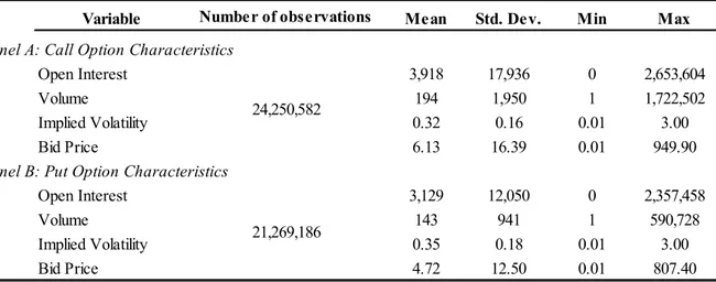
For the period under analysis, we have a total of 24,250,582 call options and 21,269,186 put options, comprising a total of 625 different firms. Table 1 reports the descriptive statistics on variables concerning put’s and call’s characteristics such as open interest, volume, implied volatility and bid price.
In our initial sample, we have more call’s than put’s contracts, with a greater volume, open interest and bid price. Focusing on their implied volatility, calls present lower values than puts, which indicates a positive call-put implied volatility spread associated with future underlying stock returns (Bali and Hovakimian, 2009; Doran, Fodor and Jiang, 2013). Nevertheless, we should not only look to the pooled avarege, and we should take into consideration other factors such as strike price, moneyness and maturity of each option contract.
Departing from call and put option data, we should focus on our measure of price pressure in the options market: the volatility spread. We created pairs of call and put options on the same underlying equity with the same strike and the same expiration date, for each day of our sample. Thus, we ended up with a sample of 11,633,684 valid option pairs across our timespan. Table 2 describes this process, from daily option data to valid option pairs, displaying the number of observations eliminated by the application of the cleaning criteria.
Afterwards, we accessed the daily data regarding the S&P500 constituents, chosen as underlying at the first stage, from CRSP (The Center for Research in Security Prices), a global
1 According to the IvyDB US Data Reference Manual, the implied volatilities of American options are calculated applying a
binomial tree. It uses the closing price of the underlying asset and the historical LIBOR/Eurodollar rates as interest rate input, and it considers the possibility of discrete dividend payments and early exercise.
database of historical stock market data. We only considered stocks with a minimum price of $5, following Cremers and Weinbaum (2010). In order to eliminate unreliable data, we eliminated stocks from our sample that have bid prices higher than, or equal to, ask prices (Goyal and Saretto, 2009; Driessen and Maenhout, 2009; Cao and Wei, 2010), and with bid prices lower than $0.125, which allows us also to minimize the impact of the tick size on bid-ask spreads (Cao and Wei, 2010). We merged the stock data – bid and bid-ask quotes, volume and number of shares outstanding – with the option data using the OptionMetrics CRSP Link provided by WRDS (Wharton Research Data Services). Lastly, we applied a filter to our sample related with the moneyness of the options considered. Following Chen, Lung and Tay (2005), we define moneyness as the ratio between the strike price of the option and the price of the underlying asset (𝐾
𝑆), setting an acceptable range of values between 0.8 and 1.2. This final filter allows us to avoid potential pricing structure issues by eliminating all the options that are far from being at-the-money (Cao and Wei, 2010)
Cremers and Weinbaum (2010) highlighted a potential relation between the deviations and higher moments of the risk-neutral distribution of underlying assets. They followed the Runbinstein (1998) procedure, specifying returns’ distribution by return, volaitlity, skewness and kurtosis. They found that more skewed distributions of the underlying asset are associated with higher option moneyness and larger volatility spreads. In a way to contribute to the reduction of the skewness effect in our research, we previously eliminated deep-in-the-money and deep-out-of-the-money options and we we conduct a winzorization process here and in section 4.2. so as to reduce the impact of the extreme value os our study variables.
The application of these criteria leads us with 10,047,532 valid option pairs for 613 unique firms. The most restricted criterion was the one related with moneyness, once eliminated more than 1.3 million of option pairs.
4. Volatility Spreads and Future Stock Returns
As discussed earlier, our main hypothesis is that deviations from put-call parity convey relevant information about future stock returns. If informed investors trade in option markets first rather than the stock market, the mechanism of information flow between the two markets and the quickness that it happens, are both a topic of interest. In order to study these, we create portfolios of stocks based on two option signals: level or level and change of the volatility
spread, and we consider the subsequent returns on those portfolios. The following section is organized as follows: firstly, we define the empirical methodology that is the base of our work; secondly, we characterize the volatility spreads of our sample; thirdly, we describe how stock portfolios are created and the method used to assess their performance; finnaly, we perform a preliminary analysis of the portfolios’ characteristics.
4.1. Empirical Methodology
Following the sequential trade model of Easley et al. (1998), buying a call or selling a put is a trade that carries positive information about future stock prices, which changes the relative price between the two option products. In a perfect market, the private information will be immediately incorporated in the underlying stock prices, and the put-call parity will be satisfied. However, in the real world, option prices can deviate from the fair values without generating a riskless arbitrage opportunity (Evnine and Rudd, 1985; Figlewski, 1989; Canina and Figlewski, 1993). This can be verified since options can be American, and be subject to transaction costs, margin requirements, taxes and differences between borrowing and lending rates (Brenner and Galai, 1986; Nisbet, 1992; Kamara and Miller, 1995). In order to determine the extent of these price distortions, we use the difference in implied volatilities between call and put options with the same maturity and strike price (Jarrow and Wiggins, 1989; Amin, Coval and Seyhun, 2004; Cremers & Weinbaum, 2010)
According with Stoll (1969) and Black and Scholes (1973), the put-call parity relation must hold in equality for European options on non-dividend paying stocks for any value of the volatility parameter (σ):
𝐶 − 𝑃 = 𝑆 − 𝑃𝑉(𝐾) (1)
∀𝜎 > 0, 𝐶𝐵𝑆(𝜎) + 𝑃𝑉(𝐾) = 𝑃𝐵𝑆(𝜎) + 𝑆, (2)
where 𝐶𝐵𝑆(𝜎) and 𝑃𝐵𝑆(𝜎) designate call and put prices according to Black-Scholes, respectively. Using the Black-Scholes pricing model, the implied volatility on a call is the number that makes the theoretical value equal to the current market price of the option (equation (3)). We get equation (4) through (2) and (3).
𝐶 = 𝐶𝐵𝑆(𝐼𝑉𝑐𝑎𝑙𝑙) (3)
𝑃 = 𝑃𝐵𝑆(𝐼𝑉𝑐𝑎𝑙𝑙) (4)
The equations (3) and (4) imply that, for a given maturity and strike price, the implied volatility of call and put options must be equal. However, with American options this is not
verified, because we have to consider the possibility of early exercise. Following Merton (1973) for American options the put-call parity should be an inequality (5).
𝑆 − 𝑃𝑉(𝑑𝑖𝑣) − 𝐾 ≤ 𝐶 − 𝑃 ≤ 𝑆 − 𝑃𝑉(𝐾) (5)
Since we have access to closing option quotes, we are only able to study deviations from the fair value and not effective violations of the relation identified in (5). Thus, we follow Battalio and Schultz (2006) and Cremers and Weinbaum (2010), and we use the difference between implied volatilities (after a correction for the dividend and early exercise effect) as merely deviations from the model. Our hypothesis is that these deviations cannot be considered pure arbitrage opportunities and that they contain relevant information about future stock performance. In an intuitive way, higher call (put) implied volatilities relative to put (call) implied volatilities indicate that calls (puts) are overpriced relative to puts (calls).
In order to measure the price pressure in the option market, we use a weighted average of the difference between call and put implied volatilities, a volatility spread (denominated as VS in the equations), following Cremers and Weinbaum (2010). As weight, we use the average trading volume of each valid option pair. Thus, we compute the volatility spread for every day
t and every stock i with put and call options data as:
𝑉𝑆𝑖,𝑡 = 𝐼𝑉𝑖,𝑡𝑐𝑎𝑙𝑙𝑠 − 𝐼𝑉𝑖,𝑡 𝑝𝑢𝑡𝑠 = ∑ 𝑤𝑗,𝑡𝑖 𝑁𝑖,𝑡 𝑗=1 (𝐼𝑉𝑗,𝑡𝑖, 𝑐𝑎𝑙𝑙𝑠 − 𝐼𝑉𝑗,𝑡 𝑖, 𝑝𝑢𝑡), (6)
where j denotes each of the 𝑁𝑖,𝑡 valid pairs of put and call options with the same maturity and strike price, 𝑤𝑗,𝑡𝑖 are weights of trading volume2, and 𝐼𝑉
𝑖,𝑡𝑘 refers to the implied volatility (k=call, put) calculated using the Black-Scholes method adjusting for early exercise and expected dividends.
As pointed out by Cremers and Weinbaum (2010), these differences between implied volatilities can be related with higher moments of risk-neutral distribution of underlying returns (particularly skewness). After applying the Rubinstein (1998) procedure, they adjusted option prices for underlying assets with nonzero skewness in order to calculate the implied volatilities through standard binomial trees. They found two important conclusions: firstly, a price pressure measure is noisier for deep-in-the-money puts; secondly, positive (negative) skewed distributions exhibit large negative (positive) volatility spread. These findings were taken into consideration in our dataset construction.
2
𝑤𝑗,𝑡𝑖 =
𝑇𝑟𝑎𝑑𝑖𝑛𝑔 𝑣𝑜𝑙𝑢𝑚𝑒𝑗,𝑡𝑖
4.2. Volatility Spreads Characteristics
In section 3 we prepared our sample satisfying a set of criteria. After that process, we are able to create daily volatility spreads for each underlying asset, by performing a weighted average3 of the difference between call and put implied volatilities of each valid option pair. From January 2003 to December 2017, our sample has 1,215,511 daily volatility spreads. We winsorized the volatility spreads at a 1% and 99% level. This last procedure eliminates larger volatility spreads (positive and negative), which are associated with negatively and positively, respectively, skewed distributions (Broadie, Chernov and Johannes, 2007; Cremers and Weinbaum, 2010).
The number of underlying assets included in the sample increases, even though not monotonically, across the timespan: the first day comprises 208 stocks and the last 434. On average, each day has volatility spreads for 322 different stocks, with a minimum of 157 and a maximum of 441 stocks in a specific day. Graph 1 shows the evolution of the number of underlying assets included in our sample for each day considered across our timeframe.
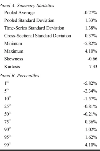
We find it useful to provide a preliminary analysis of our price pressure measure. Table 3 reports the descriptive statistics of on volatility spreads from 2003 to 2017. The mean and the median of the volatility spreads are both negative, with a value of -0.27% and -0.21%, correspondingly. According with Ofek et al. (2004) it is frequenly puts being relative more expensive than calls, translated into negative volatility spreads. In this perspective, the distribution of our price pressure, specifically the sign of the mean and median, are in line with Ofek et al. (2004) findings. Graph 2 shows the distribution of the volatility spreads – It is worth to mention that the spikes in both extremes of the graph are due to the winsorizing process conducted earlier.
The volatility spreads have a pooled standard deviation of 1.33%. The times-series standard deviation (the average, across firms, time-series standard deviation) is slightly higher, 1.38%, while the cross-sectional standard deviation (the standard deviation across firms in the time-series averages) is lower, 0.37%. This indicates a cross-sectional variation on the volatility spreads.
4.3. Formation of Portfolios and Measure of Performance
In order to test our main hypothesis, we create different portfolios of stocks based on our price pressure measure, the volatility spread, and compute the returns on those portfolios over two different investment horizons: one and four weeks. The allocation of the stocks into the respective portfolios follows two different strategies. The first uses the level of the volatility spread on Wednesdays, by splitting the sample into quintiles and then allocating the stocks into five portfolios according to the quintile to which they belong. The second strategy uses two different indicators: the change of the volatility spread from Tuesday to Wednesday, and its level on Tuesday. As before, we divide the sample into quintiles for each indicator and then we double sort the stocks according to each group created. In this way, this second strategy creates 25 different portfolios (five per level and five per change signal).
We repeat these portfolio formation processes every Wednesday using the method described above for each strategy. Afterwards, we compute the returns over the first week and over the following four weeks (this last investment horizon uses overlapping generations). The choice of Wednesday (and Tuesday in the level and change strategy) for the portfolio reallocation follows Hou and Moskowitz (2005) and Cremers and Weinbaum (2010) as a strategy to avoid the presence of noise on the returns’ measurement on Mondays and Fridays. According to Chordia and Swaminathan (2000) the returns calculated from Monday to Monday or from Friday to Friday present low and high autocorrelations, respectively. In this context, Wednesdays appear across the literature to be an adequate alternative.
Each week we only include in our portfolios stocks with at least one reported valid option pair on Wednesday and Tuesday, which enable us to guarantee reliable option signals. However we have to take into consideration the existence of a few special cases: Wednesdays (or Tuesdays) that are not trading days. For these cases, we assume the values of the nearest trading day.
When we are calculating the returns of the portfolios above mentioned, we should be aware of a potential problem: non-synchronicity, which arises with the usage of closing quotes. The stock exchange market and the options market do not close at the same time4. In this way, there is a two-minute gap between our option signal and the last stock trade, which could justify the existence of some deviations from put-call parity (Battalio and Schultz, 2006). In an effort to ensure that our results are robust and not influenced by spurious predictability, we ignore the
overnight return by computing open-to-close returns. With this procedure we use the option signal computed with the closing quote of a day, but the returns only start to accrue with the first trade of the following day, when the stock exchange market opens.
In order to compute the abnormal return of our portfolios, we use a 4-factor model (equation (6)) which includes the three Fama-French factors5 (Fama and Kenneth, 1996) and a momentum factor (Jegadeesh and Titman, 1993; Carhart, 1997). This model enables us to control for differences in risk and characteristics between the companies included.
𝑅𝑡 = 𝛼 + 𝛽1𝑀𝐾𝑇𝑡 + 𝛽2𝑆𝑀𝐵𝑡 + 𝛽3𝐻𝑀𝐿𝑡 + 𝛽4𝑈𝑀𝐷𝑡 + 𝜀𝑡, (7)
being 𝑅𝑡 the excess return over the risk-free rate, 𝑀𝐾𝑇𝑡 the excess return on the market portfolio, 𝑆𝑀𝐵𝑡, 𝐻𝑀𝐿𝑡, 𝑈𝑀𝐷𝑡, the return on three long/short portfolios that capture size, book-to-market and momentum effects, respectively.
The value of interest to measure the portfolio’s performance is the estimated value of the abnormal returns (𝛼̂). So, we run regression (7) by OLS, reporting robust standard errors for the one-week investment horizon. At the four-week frequency, the t-statistics are computed using the Newey-West autocorrelation correction6 due to the fact that we are using overlapping generations, which could lead the holding period returns to be autocorrelated up to the degree of the overlap (Cremers and Weinbaum, 2010).
4.4. Preliminary Analysis of Portfolio Characteristics
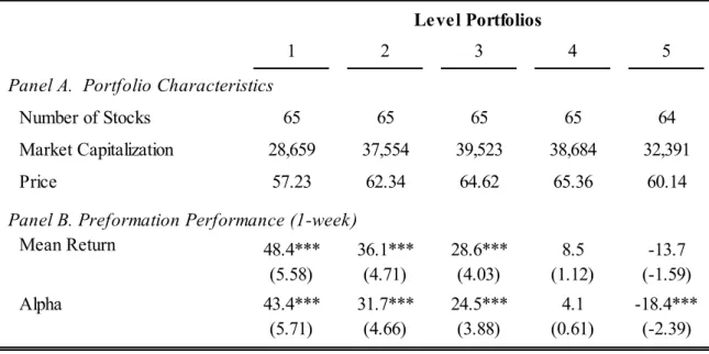
As explained in the previous section, we create weekly portfolios every Wednesday by sorting stocks into five groups based on the quintiles of the volatility spread. The number of stocks included in each portfolio varies overtime for two reasons: firstly, the S&P500 index constituents are not the same over the all timespan; secondly, options with no reported valid option pair on Wednesday and Tuesday are excluded from our sample. On average, each portfolio has 65 stocks (with a minimum of 37 and a maximum of 86 stocks), with 322 stocks overall.
Despite the fact that we are considering the largest companies listed in U.S., our sample still has some variability in the market capitalization of the companies included. If we consider only the level portfolios, the ones with greater equal-weighted market capitalization are the middle portfolios, which are the ones with lower absolute deviations from put-call parity. The stocks
5 We extract the data for all included factors from the Fama-French public database (available at
https://mba.tuck.dartmouth.edu/pages/faculty/ken.french/data_library.html).
with extreme values of volatility spreads have lower equal-weighted market capitalization, which goes in line with previous research (Easley et al. 1997). The differences between the size of the extreme portfolios, (1) or (5), and the middle one, (3), are significant at a 1% significance level.
Across the literature there are two possible explanations for this size effect. On one hand, the options written on smaller stocks can be less liquid, which can rise the transaction costs and consequently increase the arbitrage bounds. On another hand, information risk is more likely to affect smaller companies. Both liquidity and information risk effects are taken into consideration later on in our analysis.
Before we evaluate the performance of our portfolios, as described before, we do an analysis to the preformation performance of the portfolios. We use the level portfolios, with the Wednesday signal, and we measure past value-weighted returns through the preceding week. Table 4 reports the characteristics of the volatility spread quintile portfolios and their performance on the prior week to the portfolios’ formation. As we go from the portfolio with greater negative volatility spreads, (1) to the one with greater positive volatility spreads, the past abnormal returns decline. Our results indicate that call options became relatively more expensive than puts after decreases in the underlying stock. In this way, our strategy can be considered as a contrarian momentum strategy, opposing to Amin et. al (2004)who showed that volatility spreads widen following a stock market rise.
5. Performance Evaluation
5.1. Level Portfolios
Each Wednesday, we create five portfolios according to the daily level of the volatility spread. Portfolio (1) includes stocks with the lowest level of volatility spread (quintile 1) and portfolio (5) comprises stocks with the highest (quintile 5). We create also a long/short portfolio (we will name it hedge portfolio), to which we buy stocks with the high levels of volatility spread and shorts stocks with the low values (essentially, we buy quintile 5 and short quintile 1).
Afterwards, we evaluate the performance of each portfolio over the first week (1-week horizon) and also over the first 4 weeks (4-week horizon). All the calculated returns are value-weighted (not annualized), and they do not include the first overnight return, being open-close returns as previously explained. Table 5 reports the performance of the level portfolios over the
two different investment horizons. The t-stats presented are computed using robust standard errors, in case of 1-week horizon (panel A), or using the Newey-West autocorrelation correction, in case of the 4-week horizon (panel B).
The average raw and abnormal returns are positive for all portfolios, reflecting an increase as we move from the first to the fifth portfolio. Hence, we can conclude that stocks with higher volatility spreads earn higher returns than stocks with lower volatility spreads. Focusing on the hedge portfolio, over the first week it earns a value-weighted abnormal return of 13.2 bps – a value significantly different from zero at 1% significance level (t-stat of 2.85). The short side of the portfolio does not earn an abnormal return significantly different from zero (t-stat of 0.37), while the long side earns an abnormal return of 16.2 bps (significantly different from zero at 10% significance level). If we track the performance of the hedge portfolio over the subsequent four weeks, it earns a value-weighted abnormal return of 31.7 bps, also significant at a 1% significance level (t-stat of 3.61).
These results show that approximately one half of the abnormal returns, at the 4-week frequency, are due to the performance on the first week. Therefore, there is no evidence of reversal which suggests that this effect is due to information asymmetry rather than the pressure of market makers in the option’s market (for instance, as a result of delta hedging option positions in the underlying stock market).
5.2. Level and Change Portfolios
As reported by Cremers and Weinbaum (2010), there is a degree of persistence in the volatility spreads, particularly for the extreme values (among the securities they analysed, almost 25% of the them that were ranked in the tails remained there for a month). Despite the fact that we have reduced the existence of extreme values in our sample (through winsorization), it is still important to study if changes in volatility spreads carry important information besides the one conveyed by levels.
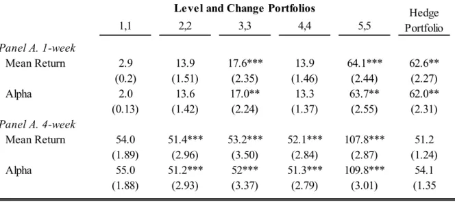
Every Wednesday, we create twenty-five portfolios in accordance with the level of volatility spread on Tuesday and the subsequent change from Tuesday to Wednesday. At Table 6 we report the performance of all portfolios built, but in this section we will only report and analyze the returns of relevant portfolios: the diagonal7 and the long-short portfolio. In this
7 For simplification reasons, the diagonal portfolios are designated by (1,1), (2,2), (3,3), (4,4) and (5,5), being 1
the portfolio with lower level (and change) and 5 the portfolio with higher level (and change) of the volatility spread.
subsection, the hedge portfolio buys stocks with both high level on Tuesday and high change from Tuesday to Wednesday, and shorts stocks with low signals, both level and change8.
Firstly, we find that the raw and abnormal returns increase with the positive extension of the signal, meaning that the high level and change portfolio (5,5) earns higher returns than the low level and change portfolio (1,1). We should notice that this increase is verified for both investment horizons, but it is not monotonic as we observed in the last subsection with the level portfolios. This finding, common to both strategies, indicates that the deviations from put-call parity are not driven by short sale constraints since the long side of the hedge portfolio earns a weekly alpha statistically different from zero (64.1 bps, with a 2.44 t-stat), which is higher than the short side (2.9 bps, not significantly different from zero).
Secondly, when both signals are taken into account at the same time the predictability degree increases. The performance of the level and change portfolios is higher than the one of the level portfolios, for both investment horizons. The hedge portfolio, based on the joint strategy, earns a weekly alpha of 62.6 bps (with a t-stat of 2.27), which is considerably higher than the 13.23 bps earned with the level strategy.
Lastly, we find that the degree of predictability decreases with the investment horizon. In this strategy, the abnormal return earned by the hedge portfolio over four weeks is no longer significantly different from zero (t-stat of 1.24), assuming a value of 51.2 bps. If we compare it with the performance of the hedge portfolio in the first week, (an alpha of 62.6 bps with a t-stat of 2.27), we see that the subsequent three weeks are not carrying any relevant performance, opposing to what we found in the prior strategy.
6. Effect of liquidity and information risk
In the previous chapters we used the deviations from put-call parity to investigate a possible information flow between the stock and the options market. We have also identified some factors that can affect the deviations, which will be our focus in this section. In this way, we will test if the level of liquidity, the existence of informed trading and asymmetric information are drivers of the identified information flow.
6.1. Option Liquidity
Starting with the liquidity effect, we study if the predictability power is impacted by the liquidity level of the option pairs. Easley et. al (1998) demonstrate that the more liquid options are the stronger will be its predictability power. From this standpoint, we first define some option liquidity measures and then we use them to build the portfolios, by sorting stocks according to the liquidity level and the option signals, as before.
6.1.1. Measures of Option Liquidity
In order to understand if the most liquid pairs have higher predictive value than the others, we construct four different measures of option liquidity: dollar ask spread, proportional bid-ask spread, contract volume and dollar trading volume (Cao and Wei, 2010).
The dollar bid-ask spread, DBA, is the difference between the closing ask and bid prices, (8). Although being the most common proxy, it is not a reliable liquidity measure for options. Keeping liquidity constant, a dollar bid-ask spread of an out-the-money option will be lower than its in-the-money counterpart. In this sense, the difference in the measure will not be due to liquidity, but to the moneyness of the option (Chordia, Roll and Subrahmanyam, 2000; Cao and Wei, 2010). Despite the fact that we will use it, we will keep this shortcoming in mind throughout the results interpretation.
DBA = 𝐴𝑠𝑘𝑗− 𝐵𝑖𝑑𝑗 (8)
The proportional bid-ask spread (PBA) is defined as the dollar bid-ask spread divided by the average price of the closing bid and ask. To use it with options we have to take a volume-weighted average of the proportional spreads within each day (9). This liquidity measure overcomes the limitation identified earlier, once it enables the comparison between options with different levels of moneyness (Chordia, Roll and Subrahmanyam, 2000; Cao and Wei, 2010).
𝑃𝐵𝐴 = ∑ 𝑉𝑂𝐿𝑗 ∗ 𝐽 𝑗=1 ∑ 𝑉𝑂𝐿𝑗 𝐽 𝑗=1 ∙ 𝐴𝑠𝑘𝑗 − 𝐵𝑖𝑑𝑗 (𝐴𝑠𝑘𝑗 + 𝐵𝑖𝑑𝑗) 2⁄ (9)
We also use two transaction-based measures: the contract volume (VOL) and the dollar trading volume (DVOL) (Hasbrouck and Seppi, 2001; Kalodera and Schlag, 2004; Cao and Wei, 2010). The first is the total number of options traded during each day (9). The second is the midpoint between the bid and ask prices weighted by the options volume (10).
𝑉𝑂𝐿 = ∑ 𝑉𝑂𝐿𝑗 𝐽
𝐷𝑉𝑂𝐿 = ∑ 𝑉𝑂𝐿𝑗 ∗ 𝐽
𝑗=1
∙ 𝐴𝑠𝑘𝑗 + 𝐵𝑖𝑑𝑗
2 (11)
6.1.2. Option Liquidity Effect – A portfolio approach
With the purpose of studying the impact of the liquidity level of an option pair in the information flow between the option and the stock market, we develop a portfolio approach based on the average liquidity of a pair and the option signals, as in previous sections. We repeat the portfolio formation process, described below, for each liquidity measure presented in 6.1.1.. Firstly, we compute the average liquidity of each option pair, after the calculation of the option liquidity, either call or put, using the four measures previously defined. Then, we construct three groups – high, medium and low liquidity – according to the terciles of each liquidity measure in that day. Hence, we compute three volatility spreads, one per each liquidity group.
After that, for each liquidity group, the process is the same as before: each Wednesday, we sort the stocks into five different portfolios according to the volatility spread quintile which they belong to. We compute open-close returns and estimate portfolios’ performance in conformity with the explained in 4.2., either for the 1- or 4-week investment horizon. The comparison between the portfolios’ performance of different liquidity groups will enable us to examine if differences in option liquidity have an impact on its informational role.
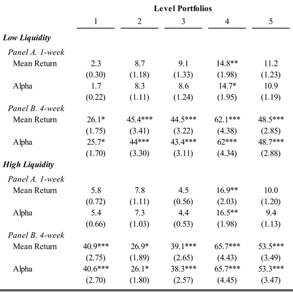
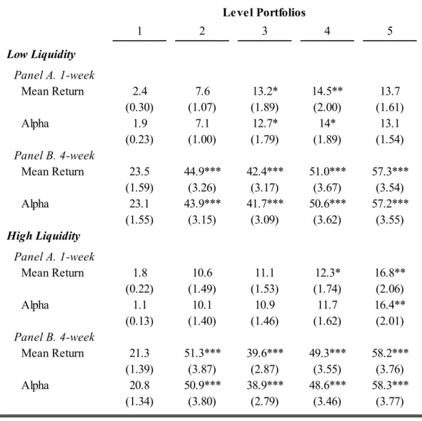
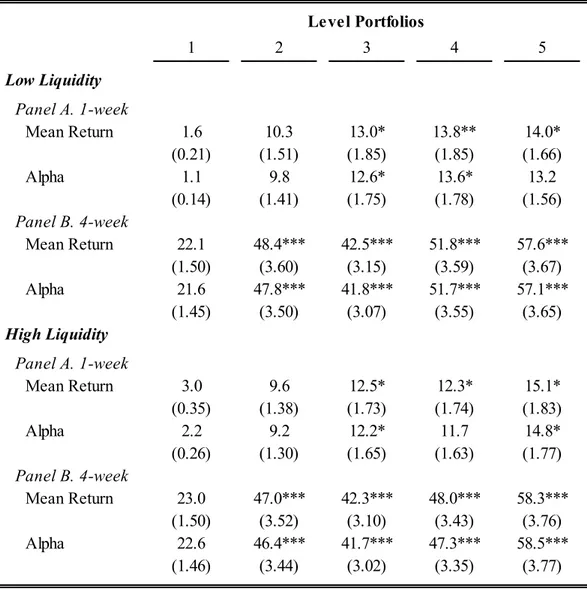
We create five level portfolios for each of the four liquidity measures presented in the previous section. However, we only analyze the results of the two most relevant, according to the literature: PBA and DVOL. The performance of the level portfolios for each liquidity group using the four measures defined is presented at Table 7.
6.2. Information Risk
Some investors have access to private information while the others only possess public information (Brown and Hillegeist, 2007). The last ones, uninformed traders, are exposed to information risk, since they will not be able to optimally choose their portfolios using all the relevant information, as opposed to informed investors (Easley, Hvidkjaer and O'hara, 2010).
In this sense, it is of our interest to study whether the deviations from put-call parity reflect the existence of informed trading. However, it is not possible to directly observe the extent of the private information. To overcome this issue, we use the probability of informed trading (PIN), developed by Brown and Hillegeist (2007), which is an extension of the EKO market microstructure model (Easley, Kiefer and O'hara, 1997). The PIN is an estimation of the probability that a trade was originated by an informed investor, according to the imbalance between buy and sell orders in the secondary market. Through the daily volume of buy and sell orders, the authors calculated PIN as follows:
𝑃𝐼𝑁 = 𝛼𝜇
𝛼𝜇 + 2𝜀 (12)
where 𝛼 is the probability of an information event, 𝜇 and 𝜀 are the trading intensity (number of trades per day) of informed and uninformed traders, respectively. By analyzing the previous equation, it is possible to take some conclusions: when private information events are more common and when the intensity of informed (uninformed) trading increases (decreases), the level of information asymmetry rises.
We retrieved the data for this measure of information asymmetry through Stephan Brown’s open database9. The previously referred author computed PINs by quarter from 1993 to 2010, using the Venter and Dejong model (Venter and De Jongh, 2006), which are more robust than the basic EKO PINs. According to Brown and Hillegeist (2007), when private information events occur with more frequency, or the trading intensity of informed trading increases, information asymmetry will arise. In contrast, it will decline with the increase of trading intensity by uninformed investors.
In order to study the characteristics of the volatility spread for a determined level of informed trading, we divide the PIN estimates into quintiles and then we allocate each volatility spread to the correspondent PIN group. At table 11 we report some summary statistics of the volatility spreads for each PIN group. We find that as the probability of informed trading increases (from
(1) to (5)), the volatility spreads become more negative and volatile, since both the average and the coefficient of variation increases in absolute value (even though, the values of the last statistics are not very different).
Despite the fact that our sample includes the largest companies traded in the US (S&P 500 constituents), we should be aware of the negative correlation between PIN and size, due to the fact that smaller companies are expected to have less liquid stocks and options (Aslan, Easley, Hvidkjaer and O'Hara, 2007). With the purpose of studying if the probability of informed trading remains a determinant of the deviations from put-call parity even for smaller and less liquid stocks, Cremers and Weinbaum (2010) run cross-sectional regressions of the volatility spreads on PIN, controlling for size and liquidity. They report that PIN continues to be a relevant determinant of the deviations.
6.2.1. Relation with Information Risk – A portfolio approach
When the share of informed investors increases, the return predictability also tends to increase (Easley, O’Hara and Srinivas, 1998). Applying this to our work, we study whether the predictability of the volatility spreads is affected by the existence of informed risk (measured by PIN).
Each Wednesday we sort stocks independently into two different categories, hence creating 25 portfolios (5x5): we create quintiles based on PIN and quintiles based on volatility spreads. Then, we measure open-close returns for the 1- and 4-week investment horizon, with weekly rebalancing.
Considering the results of the diagonal portfolios, only the portfolios that include stocks with high level of volatility spreads and high level of probability of informed trading have statistically significant abnormal returns (with 10% and 5% significance level, for 1-week and 4-week investment horizon, respectively). Table 12 shows the mean and abnormal returns of the diagonal portfolios of stocks, sorted by the level of volatility spreads and probability of informed trading (proxied by PIN).
However, in Appendix 9.9., we can see that if we keep the probability of informed trading constantly high (thus, (5)), all portfolios have statistically significant abnormal returns regardless of the level of the volatility spread on Wednesday. These results indicate that the probability of informed trading only has predictability power when combined with large volatility spreads.
7. Time-period effects
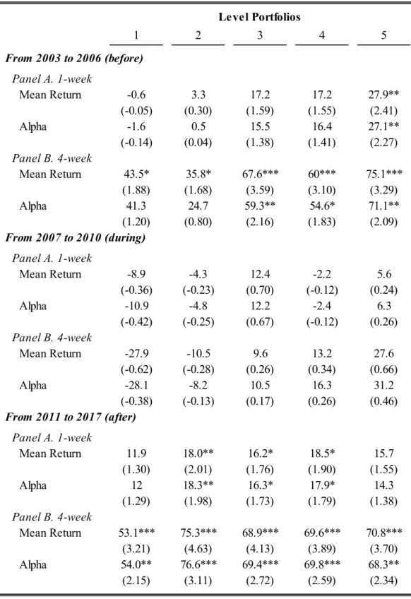
In this section we divide our sample into three groups in order to study possible differences in the information flow before, during and after the financial crisis. Then, we re-conduct the process used before with the stock portfolios’ creation using the level option signal.
Our sample period ranges from January 2003 to December 2017. This timespan covers 15 years during which the market and the economy suffered some changes, namely with the financial crisis period. These changes over our timespan can have an impact in our estimates and conclusions.
With the purpose of addressing these concerns, we create three subperiods related with the financial crisis: 2003-2006 (pre-financial crisis), 2007-2010 (financial crisis) and 2011-2017 (post-financial crisis). Afterwards, we repeat the process conducted in section 5.1., evaluating the performance of the level portfolios for each subperiod defined.
We have different results for each subperiod considered. Starting with the pre-financial crisis period (from 2003 to 2006), only the fifth portfolio (higher positive volatility spread) earns statistically significant10 positive abnormal returns for a 1-week investment horizon (27.9 bps, with a t-stat of 2.41). For a 4-week investment horizon, the third portfolio earns also a significant positive abnormal return, even though it is smaller than the return earned on the fifth (59.3 vs 71.1, both significant at 5% significance level). Proceeding to the financial crisis period (from 2007 to 2010), the returns reported are all lower than the ones presented in the previous period, being all not statistically different from zero. Lastly, considering the portfolios built in the post-financial crisis (from 2011 to 2017), all of them earn statistically significant abnormal returns over 4-weeks, with the majority of the portfolios earning returns higher than the ones earned in the pre-financial crisis. Additionally, over the first week, the middle portfolios (lower volatility spread) seem to have higher predictability power than in its previous periods.
Overall, our results show that the volatility spreads have a higher predictability power in the post-financial crisis period, mainly for the 4-week investment horizon. These goes against Cremers and Weinbaum (2010) findings: they identified a reduction of the return predictability degree of volatility spreads, considering a sample period from January 1996 to December 2005.
10 With a 5% significance level
8. Conclusion
In our work we study the contribution of the option market to the price discovery process in the stock market. Specifically, we study the existence of information about future stock prices intrinsic to the deviations from put-call parity, a well-known relation between calls, puts and stock prices. The existence and the dynamics of the information flow between the option and the stock market is not consensual across the literature: some argue that it is due to the existence of short-sale restrictions, higher leverage, informed trading or prevalence of asymmetric information. The foundation argument of our work is that informed trading leads to the contribution, by the stock market, to the price discovery process in the stock market.
As a measure of price pressure in the option market, we use the volatility spread which is the volume-weighted average difference between the implied volatility of a call and the implied volatility of a put for the same maturity, underlying stock and strike price. We focus on the largest market capitalization companies in the U.S., considering only options whose underlying asset is a stock constituent of the S&P 500 index. Each Wednesday, we create stock portfolios based on some characteristics of the volatility spreads (level, change and liquidity) and of the option market (probability of informed trading).
Our results indicate that stocks with higher positive volatility spreads outperform stocks with lower and negative volatility spreads, meaning that relatively expensive calls in respect to puts carry more information about future stock returns than the other way around. Firstly, we use two different investment strategies: one based on the level of the volatility spread and other based on its level and change. Both hedge portfolios built earn value-weighted abnormal returns over, at least, the first week of investment, confirming the conclusion identified before. Secondly, we extend our analysis to study if different levels of options’ liquidity and probability of informed trading have influence on the future stock return predictability. We identified a positive relation in both factors: more liquid options and higher probability of informed trading induce a higher informational flow between the option and the stock market. Contrary to Cremers and Weinbaum (2010), we don’t document a decrease of the predictability degree over the sample period, since the portfolios created in the latest years of our sample (post-financial crisis period) earn higher returns than the earlier ones.
Nevertheless, our analysis has some shortcomings representing possible extensions for future research. Firstly, we conduct a winsorization process to eliminate the extreme values of the volatility spreads, which can lead us to ignore some important information carried by the
options with highest deviations from put-call parity. Secondly, to compute the abnormal returns we lack to control for skewness risk. Positively and negatively skewed distributions can be responsible for generating positive and negative volatility spreads. However this effect is most prominent on large differences in implied volatilities (some of them, we eliminate from our sample due to the winsorization process). Thirdly, for the study of the informed trading presence in the option market, the PIN data is only available until 2010, which reduces the sample to almost one half the initial one. Moreover, future research in this field could include the investigation on the effect of different levels of options’ moneyness and stocks’ liquidity. Finally, it would be worthwhile to explore the information flow between the two markets around important company information releases, for example earnings announcements, or the publication of analysts’ recommendations.
9. References
Amin, K., Coval, J. D., & Seyhun, H. N. (2004). Index Option Prices and Stock Market Momentum. The Journal of Business, 77(4), 835-874.
Anthony, J. H. (1988). The Interrelation of Stock and Options Market Trading‐Volume Data.
The Journal of Finance, 43(4), 949-964.
Aslan, H., Easley, D., Hvidkjaer, S., & O'Hara, M. (n.d.). Firm Characteristics and Informed Trading: Implications for Asset Pricing.
Atilgan, Y. (2014). Volatility spreads and earnings announcement returns. Journal of Banking
& Finance, 38, 205-215.
Bali, T. G., & Hovakimian, A. (2009). Volatility spreads and expected stock returns.
Management Science, 55(11), 1797-1812.
Battalio, R., & Schultz, P. (2006). Options and the bubble. The Journal of Finance, 61(5), 2071-2102.
Bhattacharya, M. (1987). Price Changes of Related Securities: The Case of Call Options and Stocks. Journal of Financial and Quantitative Analysis, 22(1), 1-15.
Black, F. (1975). Fact and Fantasy in the Use of Options. Financial Analysts Journal, 31(4), 36-41.
Black, F., & Scholes, M. (1973). The pricing of options and corporate liabilities. Journal of
Political Economy, 637-654.
Bollen, N. P., & Whaley, R. E. (2004). Does net buying pressure affect the shape of implied volatility functions? The Journal of Finance, 59(2), 711-753.
Booth, G. G., So, R. W., & Tse, Y. (1999). Price discovery in the German equity index derivatives markets. Journal of Futures Markets: Futures, Options and Other Derivative
Products, 19(6), 619-643.
Brenner, M., & Galai, D. (1986). Estimation of errors in the implied standard deviation. Salomon Bros. Center for the Study of Financial Institutions, Graduate School of Business
Administration, New York University.
Broadie, M., Chernov, M., & Johannes, M. (2007). Model specification and risk premia: Evidence from futures options. The Journal of Finance, 62(3), 1453-1490.
Brown, S., & Hillegeist, S. A. (2007). How disclosure quality affects the level of information asymmetry. Review of Accounting Studies, 12(2-3), 443-477.
Canina, L., & Figlewski, S. (1993). The Informational Content of Implied Volatility. Review of
Financial Studies, 6(3), 659-681.
Cao, M., & Wei, J. (2010). Option market liquidity: Commonality and other characteristics.
Journal of Financial Markets, 13(1), 20-48.
Carhart, M. M. (1997). On persistence in mutual fund performance. The Journal of Finance,