A Work Project, presented as part of the requirements for the Award of a Master Degree in Economics from the NOVA – School of Business and Economics
PRICES, MONEY AND THE EXCHANGE RATE IN ANGOLA: AN ANALYSIS OF THE RELATIONSHIPS
LUIS TOMÁS RIBEIRO ROSA ACUÑA 3078
A PROJECT CARRIED OUT ON THE MASTER IN ECONOMICS PROGRAM, UNDER THE SUPERVISION OF:
PROFESSOR MIGUEL LEBRE DE FREITAS
Abstract
Since 2014, the Angolan economy has been under heavy instability due to the falling of international oil prices. To fight inflation, the National Bank of Angola is now using, as instruments, the exchange rate and money supply. This Work Project uses a Vector Error Correction model to assess which one is more effective in influencing CPI inflation. We do so using the Johansen procedure, where we identify two cointegrating vectors. One for the money market equilibrium and the other capturing the Dutch Disease. The analysis performed finds evidence that supports the nominal exchange rate as the most impactful tool to contain inflation.
I. INTRODUCTION
Since 2003, Angola has maintained a fixed peg of its Kwanza (AOA) against the United States Dollar (USD). In parallel, the trajectory followed by the terms of trade facing Angola has been positive. As a consequence, the Angolan economy has suffered a process of real exchange rate appreciation that ended up leaving it as one of the most expensive economies in the world. Angola is one of the biggest oil producers in Africa and oil exports represent more than 90% of its annual exports. Thus, rising oil prices across almost all the period that is covered in this Work Project (WP) are certainly a part of the explanation for the observed sky rocketing prices in Angola, in what is a clear manifestation of the Dutch Disease (Corden and Neary, 1982). Various authors have published research on the Angolan inflation phenomenon. The three main benchmarks for this WP will be Lariau, El Said and Takebe (2016), Klein and Kyiei (2009) and Gelbard and Gelbard and Nagayasu (2004). The first uses a Vector Error Correction (VEC) model and identifies one long run relationship between the exchange rate, the price level and the import prices. The second does also use a VEC model but identifies two long run relationships, the first between prices and exchange rate and the second between GDP and money supply. The third is slightly different since it focuses solely on the determinants of the real exchange rate. The authors find evidence of the Dutch Disease, estimating only one vector for the relationship between real exchange rate, oil prices and foreign interest rate. Finally, the International Monetary Fund (IMF) 2003 Selected Issues and Statistical Appendix for Angola present a clear road to study the inflation path. The authors start by performing bivariate granger causality tests. Then move to a differenced VAR to compute IRFs and FEVDs. These two steps are meant to start grasping the variables interrelationship. Finally, an error-correction model is estimated using money, the exchange rate and prices.
This WP presents two long run relationships in its VEC model. The first relates the exchange rate and oil prices by the real exchange rate equation (as suggested by the Dutch Disease) and the second relates money and prices by the money market equilibrium equation. Together, they compose the monetary approach. In comparison with previous literature, this approach has been deemed the most appropriate to deal with the above mentioned two sources of inflation pressures, to analyze them separately and to address the monetary equilibrium in a more complete framework. Concretely, we try to follow IMF (2003) when building towards the VEC model. In the VEC model, we follow Klein and Kyiei (2009) dual approach to inflation and we enrich it with a real exchange rate equation, like Nelbard and Nagayasu (2004) did.
The WP continues as follows: Section II develops the theory and literature related with the purpose of the dissertation. Section III describes the methodologies chosen and the data set that was used. Section IV displays the results of the Granger Causality tests, the results (Impulse Response Functions, IRFs, and Forecast Error Variance Decompositions, FEVDs) of the Vector Autoregressive (VAR) model and the results of the VEC model. Finally, Section V concludes.
II. THEORY AND LITERATURE
The approach that this WP will follow to describe the fashion in which money and exchange rates influence the price level will be based in two equations.
The first is the demand and supply equality in the money market. Here, real money demand is defined as a positive function of real GDP (the variable that represents volume in the economy) and a negative function of inflation (that represents the opportunity cost of holding money). This is a Money Demand function á la Cagan (1956). In an economy subject to high rates of inflation and controlled interest rates that often turn negative in real terms, such as the Angolan one, inflation expectations are an appropriate measure for the opportunity cost of holding money.
The second relationship involves the real exchange rate and the terms of trade. In the case of Angola, oil exports represent more than 90% of Angola’s exports. When oil prices increase, revenues for Angola increase as well. Causing an accumulation of foreign reserves and a demand expansion. This demand expansion increases prices for non-tradables. The end result is that the real exchange rate appreciates (note that the nominal exchange rate in Angola was mainly fixed along the sample used).
III. DATA AND METHODOLOGY A. Methodology
To assess the inflation phenomenon in Angola, the VEC model was chosen. The VEC model has the ability to distinguish between the long run relationship of the variables and their short run dynamics. Previous to this VEC, Granger Causality tests were performed and a VAR model was built in order to start grasping how the price level, the monetary aggregates and the exchange rates influence each other (as in IMF, 2003). However, since the VEC model will be the touchstone of this WP, let us explain its features as in Enders (1980):
N variables can be in long run equilibrium such that:
𝛽"𝑥"$+ 𝛽'𝑥'$+ 𝛽(𝑥($+ … + 𝛽*𝑥*$ = 𝑒$ ; 𝑒$ being the deviation from equilibrium Usually, some normalization is made to have one variable as a function of the others:
𝛽 = 1 −𝛽' −𝛽( … −𝛽*
These n variables need to have the same order of integration and a linear combination of them needs to be I(0). This long run relationship is the cointegrating relationship. 𝛽 is the cointegrating vector.
and P-lags example to perceive how the model incorporates short term reactions to long run equilibrium deviations. A cointegrating relationship between y and c exists as follows:
1𝑦$− 𝛽"𝑐$ = 𝜀$ ; such that: 𝑦$− 𝛽"𝑐$= 𝜀$ ; Note that: 𝑦$3"− 𝛽"𝑐$3" = 𝜀$3" Generalizing to P lags, the matrix form of the VEC model would be as follows:
∆𝑦$ ∆𝑐$ = 𝑎"6 𝑎'6 + −𝛼𝛼;8(1)(1) −𝛼𝛼;8(−𝛽(−𝛽"")) 𝑦𝑐$3"$3" + =?">3" 𝑎𝑎'"""(𝑖) 𝑎(𝑖) 𝑎"'''(𝑖)(𝑖) ∆𝑦∆𝑐$3=$3= + 𝜀8@ 𝜀;@ Generalizing to N variables, the VEC model (as a matrix equation) would look like this: ∆𝑥$= 𝜋B + 𝜋𝑥$3" + >3"=?" 𝜋=∆𝑥$3= + 𝑒$
Now that the dynamics behind the VEC model have been explained, we will proceed to the explanation of the Johansen methodology that allows for model testing and estimation. The first step is to check all the variables for their order of integration to guarantee that all have the same one1. Once this is confirmed, lag length tests on Standard VARs (with the undifferenced data) should be made until the longest reasonable one. The Likelihood Ratio (LR) test statistic is preferable, although the Schwarz Information Criterion (SIC) and the Akaike Information Criterion (AIC) are good alternatives, for lag selection.
The second step requires the model to be estimated. Assuming that LR = SIC = AIC = 2, an estimated 3-variable model would be as follows:
∆𝑥$ = 𝜋B + 𝜋𝑥$3" + 𝜋"∆𝑥$3" + 𝑒$
One should always check the residuals to guarantee they are white noise. Assuming that they
are, the number of cointegrating vectors (r, the rank of p) that can be built from the variables in 𝑥$ must be found. Two statistics can be used for this, 𝜆$DE;F and 𝜆GEH.
The third step is the estimation of the VEC model. Assuming that the previous step yielded that there is 1 cointegrating vector, we should end up with the already mentioned two parts of the model. One for the long run equilibrium and one for the short run dynamics.
Assuming that the coefficients of the estimated long run equation are: 𝛽6 ; 𝛽" ; 𝛽' ; 𝛽( = ( 0,01 ; 0,42 ; 0,43 ; −0,42)
Normalizing: ( -0,02; -1; -1,02;1). To test the joint restriction (0; -1; -1 ;1), its 𝜒' value must be calculated and compared against its critical value. In the case of our model, we will want to test the following restrictions:
First vector:
(𝛽6 , 𝛽OPQR , 𝛽STS , 𝛽UOV , 𝛽W6 , 𝛽TX, 𝛽V*YZE$=B*) = (𝛽6 , 1, 𝛽STS > 0 , −1, 0, 0, 0) Second vector:
(𝛽6 , 𝛽OPQR , 𝛽STS , 𝛽UOV , 𝛽W6 , 𝛽TX, 𝛽V*YZE$=B*) = (𝛽6 , 0, 0, −1, 1, 𝛽TX< 0, 𝛽V*YZE$=B* > 0) Finally, the fourth step requires causality tests and innovation accounting procedures (IRFs and FEVDs) to be taken in order to identify a structural model and determine if the estimated model is appropriate.
B. Data
To study the inflation phenomenon in Angola, monthly observations from January 2007 to December 2014 were used. This way, the sample was isolated from the post war instability
period (the Civil War ended in April 2002) and also from the instability that took over the Angolan economy after the oil prices started falling in the second semester of 2014. Moreover, this WP analyses the period subsequent to 1997-2007, studied by Klein and Kyei (2009). The variables chosen to perform this analysis are the Consumer Price Index (CPI), the Nominal Exchange Rate (NER), the Parallel Nominal Exchange Rate (PNER)2, the Money Supply (M0 and M2), the Terms of Trade (TOT) and the Oil Exports (OX)3. CPI, NER and OX were obtained from the National Bank of Angola (BNA). Money Supply was obtained from the IMF’s International Financial Statistics (IFS) database. TOT was obtained from the IMF’s IFS database (Euro Area’s CPI, the assumed price of Angola’s imports) and from the United States Energy Information Administration (Brent crude oil price, the assumed price of Angola’s exports). PNER was obtained from informal sources. NER is set administratively. As a consequence, along this WP, PNER will be experimented as well as the official one.
One of the greatest challenges of this WP was to deal with the lack of sources from which to obtain observations for variables that would help to better understand inflation in Angola. Fortunately, everything weighted in, the feeling is that proper variables were still found and that the size of the sample (96 observations per variable) is also very much acceptable.
IV. RESULTS
A. Order of Integration
To assess the rules of integration of the variables, two types of tests were performed. The Augmented Dickey-Fuller (ADF) test and the Philips Perron (PP) test. The maximum number
2 The PNER sample was incomplete in years 2005 and 2010 and in the first 5 months of 2009. As a consequence,
PNER values for these months were interpolated using the cubic spline method with multiplicative option.
of lags selected was 12 and the SIC was the chosen criterion. The starting point was to test all the variables in natural logs. As expected, the null hypothesis could not be rejected for none of the variables at the 1% significance level. The only note of concern goes to Inflation, although the null hypothesis could not be rejected when using the AIC. Moving forward, all the variables in first differences of the natural logs were also tested for stationarity. For the first differences, the alternative hypothesis of stationarity could not be rejected at the 1% significance level. In order to reinforce these findings, PP tests were also carried out. Two features must be selected in order to perform the test, the spectral estimation method and the bandwidth automatic selection method. In this case, Barlett Kernel and Newey-West were chosen, respectively. The results were the same as the ones obtained using the ADF test. Consequently, stationarity will be assumed for the first differences of all the variables in question.
B. Granger Causality
After all the series were checked for their order of integration bivariate Granger Causality tests were performed to start understanding the relationship between the variables and its significance. Several variables were included when running these tests: CPI, monetary aggregates (M2 and M0) and nominal exchange rates (parallel and official). The table that follows (Table 1) specifies which lags are significant at the 5% significant value.
Table 1: Granger Causality Tests
The parallel nominal exchange rate seems to be a good predictor of M0 across several lags. The official nominal exchange rate, on the other hand, seems to be a good predictor of M2. This is probably due to the fact that M2 is a measure that includes foreign currency deposits, which have an important weight in the Angolan banking system. Reversely, the parallel nominal exchange rate can be again very much affected by shifts in M0. The official nominal exchange rate seems more disconnected from the monetary aggregates and just responds with some lags. This is probably due to its administrative nature; the parallel nominal exchange rate seems to better reflect market conditions.
Concerning the CPI. Results tell us that the monetary aggregates do not help in forecasting CPI. Moreover, the parallel nominal exchange rate does not seem to help either. The only variable that appears to be a good predictor of future CPI values is the official nominal exchange rate. This result is puzzling given that during the 2007-2014 period, the two exchange rates move basically together. In any case, there is only one lag at which this granger causality relationship is significant at the 5% level. The VAR model will allow for a more complete analysis.
C. VAR
Before moving to the VEC model, a standard VAR model was estimated. This tool permits the examination of the relationship between the monetary aggregates, the exchange rates and CPI with more detail considering all the variables as endogenous and accounting for feedback effects. Appendix 1 and Appendix 2 contain the graphs for the IRFs and the FEVDs.
Concerning the IRFs, results show that CPI responds positively, as expected, to shocks in both M0 and M2. Shocks to NER and PNER do also generate positive responses from CPI, as expected as well. However, the response magnitude is very low. CPI responds significantly only to shocks in its own past values. See Appendix 1.
Concerning the FEVDs, some of the insights derived from the IRFs are reinforced. The CPI is mostly affected by its own past values. The monetary aggregates and the PNER do not represent more than 5% of the forecast error variance of CPI at any point in time and NER reaches only 8%. See Appendix 2.
Results are rather weak, which is understandable given that the estimation only considers the variables in differences. Still, together with the granger causality analysis and the IRFs, we may draw some conclusions: CPI responds as expected to the shifts in exchange rates and in monetary aggregates which evidences its link with both kinds of variables. Moreover, links with the official nominal exchange rate seem stronger when looking at all the results and CPI is also mostly related to its own past values which are indicators of a situation of some stability.
D. VEC
The combination of a monetary aggregate and an exchange rate variable that allowed us to achieve two vectors of the required form was M0 and PNER. In this way, theoretical conceptions regarding the real exchange rate equation and the monetary economy equilibrium would be respected and the model could be observed according to them.
Before analysing the results, another remark should be made about the lag length of the model. The lag length chosen was 2 according to the AIC, the SIC, the LR, the Hanan-Quinn criterion and the Final Predicted Error criterion. These criterions were applied to VAR models with all the variables in logs (undifferenced). Moreover, a lag length of 2 was the minimal lag length that ensured no serial correlation. However, residual homoscedasticity and normality could not be guaranteed. As normality does not raise any important question, homoscedasticity might (regarding parameter significance, for instance). As such, results of the model must be read in the light of this fragility. Results of the lag length, serial correlation, homoscedasticity and normality tests can be found in Appendixes 3, 4, 5 and 6, respectively.
However, the validity of the model should also be assessed through the cointegration test. As it can be seen as follows (Table 2), identifying restrictions are not rejected by the test statistics.
Table 2: Cointegration Tests
This estimated VEC model provides us with various insights (Table 3). First of all, the restrictions pass the LR test (Table 4). This means that, in the long run, exchange rate pass-through to prices is complete and money is neutral. These two results confirm the suitability of the monetary approach for the Angolan inflation case. Moreover, TOT has the expected sign and is significant. This supports the Dutch Disease argument for the determinants of the Angolan real exchange rate. Then, OX and Inflation do also present the expected signs. Nonetheless, while Inflation is significant, OX is not. Inflation proves to be a good measure for the opportunity cost of holding money while OX may not such a good proxy for GDP. Still, the sign of its coefficient is in line with theory.
Table 3: Identification of Long Run Relationships
Table 4: LR Test for Binding Restrictions
Table 5: Adjustment Coefficients
Regarding the short run dynamics (Table 5), restrictions in the not significant adjustment coefficients were not rejected. Both error-correction terms facing D(CPI) have the expected sign (positive, CPI rises with a Kwanza depreciation or with an M0 expansion) and are significant. Moreover, non-significance found in the PNER adjustment coefficient from the real exchange rate equation leads us to strike CPI as the main adjuster to deviations from long run
equilibrium. However, the magnitude of the coefficient indicates a slow adjustment. Non-significance found in M0, OX and Inflation adjustment coefficients from the monetary equilibrium equation also leads us to strike CPI as the main adjuster to deviations from long run equilibrium. The adjustment is again very slow. In fact, the CPI adjustment to the real exchange rate equation, although slow, is much faster than its adjustment to the monetary equilibrium equation. Moreover, D(PNER) lags are the lags that affect D(CPI) with the greatest magnitude (Appendix 7). It appears that, in the short run, exchange rate movements are much better explainers of CPI behaviour than money supply shifts.
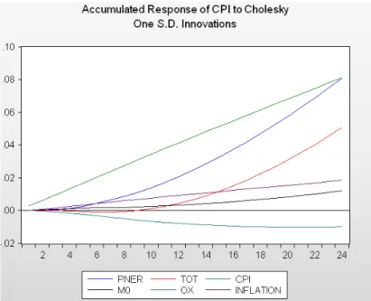
Figure 1: Accumulated CPI IRFs
To complete this analysis, let us look at the IRFs and FEVDs (Graphs 1 and 2). The IRFs confirm the already mentioned preponderance of the exchange rates in determining CPI. CPI responds accordingly to M0 as well but with much less strength. Another mention should go for TOT that also affects CPI positively, reflecting the Dutch Disease.
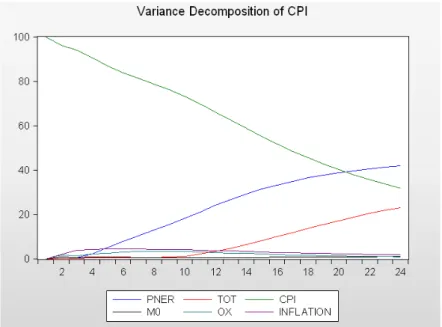
Figure 2: CPI FEVD
Finally, looking at the FEVDs, more evidence is found to support PNER as the main explainer of the CPI behaviour. After one year, it attains about 20% of the variance decomposition.
V. CONCLUSIONS
The work developed along this WP builds towards the demonstration of the existence of a long run relationship between the variables in the real exchange rate equation (enriched with Corden and Neary (1982) propositions) and between the variables in the real money equation (according to the Cagan model). These two equations generally support the Monetary Approach. Given that, the focus goes to explore which factors determine the CPI path. CPI adjusts significantly to deviations from both equations. Looking at the magnitudes of the coefficients, most attention goes to parallel nominal exchange rate. IRFs and FEVDs present strong evidence of its distinct role in determining inflation.
Lariau, Moataz and Takebe (2016) find that 1 percent depreciation of the AOA against the USD leads to a 0,64 percent increase in the price level (in the long run). This WP does not reject that this 1% depreciation leads to a 1% increase in the price level. In the short run, however, the
price level lacks adjustment. The authors justify this divergence with the administrative nature of pricing in various markets. In contrast, this WP finds that the price level adjusts significantly in the short run.
Klein and Kyiei (2009) find that there is a significant short run adjustment of the price level to deviations from the equilibrium exchange rate. Moreover, the size of the coefficient shows that this adjustment is made in three or four quarters. Adjustment in our WP seems slower, which might be due to the more stable period that this WP studies. As of the vector reflecting the monetary part of the economy, the price level seems to be affected mainly through the nominal GDP coefficients. The lack of adjustment from CPI may be due to a less specified monetary equation that does not take into account the opportunity cost of holding money, as well as the relevance of the price level itself to the monetary equilibrium.
Finally, IMF (2003) finds that both the exchange rate and monetary aggregates are significant but that none passes completely to the price level, in the long run. This is natural given that both variables are included in the same cointegration equation. This WP approach allows for defining the impact of both variables through two different equations.
In the light of the recent drop in international oil prices, Angolan authorities should be careful on how to deal with the nominal exchange rate. The terms of trade facing Angola suffered an important depreciation and, as a consequence, so will the real exchange rate. This will require nominal depreciation to avoid a fall in CPI. We have seen that a nominal depreciation has the ability to rise prices.
It is also important that a deviation from long run equilibrium between real money supply and demand causes CPI to adjust and grow. The adjustment coefficient is limited but it is still significant. The nature of this adjustment coefficient should be interpreted as a red flag when we look at the growing path of M0 and M2 during the period covered in this WP.
VI. REFERENCES
Al Raisi, A. H. & Pattanaik S. 2005. Pass-Through of Exchange Rate Changes to Domestic Prices in Oman. CBO Occasional Paper.
Aron, J., Macdonald, R. & Muellbauer, J. 2004. Exchange Rate Pass-Through in Developing and Emerging Markets: A Survey of Conceptual, Methodological and Policy Issues, and Selected Empirical Findings. The Journal of Development Studies.
Billmeier, A. & Bonato, L. 2002. Exchange Rate Pass-Through and Monetary Policy in Croatia.
IMF Working Paper.
Burstein, A. & Gopinath, G. 2013. International Prices and Exchange Rates. NBER Working
Paper.
Dreger, C. & Wolters, J. 2010. Investigating M3 money demand in the euro area. Journal of
International Money and Finance.
Enders, W. 1980. Applied Econometric Time Series. John Wiley and Sons.
Gelbard, E. & Nagayasu, J. 2004. Determinants of Angola’s Real Exchange Rate, 1992-2002.
The Developing Economies.
Hyder, Z. & Shah, S. 2004. Exchange Rate Pass-Through to Domestic Prices in Pakistan. SBP
Working Paper.
Klein, N. & Kyiei, A. 2009. Understanding Inflation Inertia in Angola. IMF Working Paper. Lariau, A., El Said, M. & Takebe, M. 2016. An Assessment of the Exchange Rate Pass-Through in Angola. IMF Working Paper.
Laryea, S. A. & Sumaila, U. R. 2001. Determinants of Inflation in Tanzania. CMI Working
Paper.
McCarthy, J. 2000. Pass-Through of Exchange Rates and Import Prices to Domestic Inflation in Some Industrialized Economies. Federal Reserve Bank of New York Research Paper. McFarlane, L. 2002. Consumer Price Inflation and Exchange Rate Pass-Through in Jamaica.
Bank of Jamaica Research Paper.
Ocran, M. K. 2010. Exchange Rate Pass-Through to Domestic Prices: The Case of South Africa. Prague Economic Papers.
Ogundipe, A. A. & Egbetokun, S. 2013. Exchange Rate Pass-Through to Consumer Prices in Nigeria. Journal of Business Management and Applied Economics.
Pastor, G. et al 2003. Angola: Selected Issues and Statistical Appendix. IMF Country Report. Rowland, P. 2004. Exchange Rate Pass-Through to Domestic Prices: The Case of Colombia.
Banco de la República ESPE Review.
Sanusi, A. R. 2010. Exchange Rate Pass-Through to Consumer Prices in Ghana: Evidence from Structural Vector Auto-Regression. MPRA Paper.
VII. APPENDIX Appendix 1
Appendix 2
Appendix 4
Appendix 5