Energy efficient adsorption processes for environmental applications

(1)

Energy efficient adsorption processes for

environmental applications

Master’s Thesis

by

Luís Alberto Macedo e Rocha

SINTEF – Materials and Chemistry

FEUP Supervisor: Prof. Adélio Mendes SINTEF Supervisor: Dr. Carlos Grande

Departamento de Engenharia Química

(2)

(3)

(4)

(5)

Acknowledgments

I would like to show my sincere gratitude to my supervisors Dr. Carlos Grande at SINTEF and Professor Adélio Mendes at FEUP, for allowing me to take part in this project and for all their help and availability during this internship. Thanks to them I was able to learn a lot during these 5 months and interact with an exciting work.

To Mahdi Abdollahzadeh I would like to acknowledge the help and suggestions given during the development of the mathematical model and numerical methods.

To my family and friends I would like to express my gratitude for all the support, motivation and friendship throughout all the work on this thesis.

The support of the Research Council of Norway through the CLIMIT program by the SINTERCAP project (233818). This publication has been produced with support from the BIGCCS Centre, performed under the Norwegian research program Centres for Environment-friendly Energy Research (FME). The author acknowledges the following partners for their contributions: ConocoPhillips, Gassco, Shell, Statoil, TOTAL, GDF SUEZ and the Research Council of Norway (193816/S60).

(6)

(7)

Abstract

CH4/CO2 separation is relevant for the treatment of natural gas. Among the different

technologies employed nowadays to ensure that separation, adsorption has become more important and has plenty of potential for improvement. In this work, the carbon molecular sieve KP – 407 was studied for the separation of a stream of 90 % methane and 10 % carbon dioxide. The equilibrium and kinetic properties of the adsorbent were studied based on adsorption equilibrium isotherms, uptake curves and breakthrough curves.

The adsorption isotherms of carbon dioxide and methane were measured at 298 and 343 K and fitted with the multisite Langmuir model; the adsorbent displays a slightly greater affinity towards CO2 compared with methane. The uptake curves were analysed to determine the kinetic

properties of the two components; carbon dioxide diffuses much more rapidly through the micropores of the adsorbent than methane. Methane presents an additional constriction at the pore mouth having an important contribution towards the overall resistance to CH4 diffusion.

Breakthrough curve experiments were performed at pressures from 5 to 70 bar in order to simulate the high pressure conditions of natural gas handling. A comprehensive phenomenological model to describe these experiments was detailed and was used to simulate the breakthrough curves. These experiments suggest that further work is necessary since the regeneration of the column during the fixed bed experiments was not complete.

Therefore, this work provides the description and implementation of a sophisticated mathematical model for the simulation of a fixed bed adsorption column and the analysis of experiments on adsorption equilibrium, kinetics and breakthrough curves. In addition, it presents the study of a new adsorbent and its behaviour at pressures as high as 70 bar.

(8)

(9)

Resumo

A separação CH4/CO2 é relevante no tratamento de gás natural. Entre as diferentes

tecnologias empregues nos dias de hoje para assegurar essa separação, a adsorção tem-se tornado uma das mais importantes e com maior potencial de evolução. Neste trabalho, a peneira molecular de carbono KP – 407 foi estudada para a separação de uma corrente de 90 % de metano e 1 0% de dióxido de carbono. O equilíbrio e cinética desses componentes neste adsorvente foram estudados, juntamente com experiências de curvas de rutura a diferentes pressões.

As isotérmicas de adsorção foram medidas a 298 e 343 K, tendo sido ajustadas com o modelo multisite Langmuir. O adsorvente demonstrou uma maior afinidade para com o CO2,

apesar da baixa seletividade de equilíbrio. As curvas de uptake foram analisadas para determinar os parâmetros cinéticos dos componentes. O dióxido de carbono difunde-se através dos microporos muito mais rapidamente que o metano, sendo que a constrição na entrada dos poros tem uma contribuição importante na resistência à difusão deste componente.

Experiências de curvas de rutura foram realizadas a pressões desde 5 até 70 bar, de modo a simular as condições de alta pressão no manuseamento de gás natural. Um modelo matemático para descrever estas experiências é detalhado e utilizado em simulações. Estas experiências sugerem que trabalho adicional é necessário para descrever e simular a cinética dos compostos envolvidos nesta separação.

Assim, este trabalho apresenta a descrição de um detalhado e sofisticado modelo matemático para a descrição de curvas de rutura juntamente com experiências de equilíbrio, cinética e leito fixo. As propriedades de um novo adsorvente são desta forma apresentadas a pressões até 70 bar.

(10)

(11)

Official Statement

I declare, under honor commitment, that the presente work is original and that every non original contribution was properly referred, by identifying its origin.

(12)

i

List of Figures

Figure 4.1 – Experimental PSA unit used for the fixed bed experiments ... 19

Figure 4.2 – Simplified diagram of the experimental setup used for the breakthrough curve experiments.. ... 25

Figure 5.1 – Adsorption isotherms of CH4 ... 25

Figure 5.2 – Adsorption isotherms of CO2 ... 25

Figure 5.3 – Virial plots for methane.. ... 25

Figure 5.4 – Virial plots for carbon dioxide. ... 25

Figure 5.5 – Carbon dioxide isotherms as a single component and in a system with 90 % methane and 10 % carbon dioxide.. ... 25

Figure 5.6 – Methane isotherms as a single component and in a system with 90 % methane and 10 % carbon dioxide. ... 25

Figure 5.7 – Adsorption kinetics of CO2 and CH4. ... 25

Figure 5.8 – Adsorption kinetics of CO2 and CH4 over the square root of time.. ... 25

Figure 5.9 – Adsorption kinetics of CH4 at 298 K with the solid lines representing the mathematical models.. ... 25

Figure 5.10 – Adsorption kinetics of CO2 at 298 K with the solid line representing the mathematical model. . ... 30

Figure 5.11 – Breakthrough curves (left) and temperature histories (right) at 5 bar.. ... 31

Figure 5.16 – Breakthrough curves (left) and temperature histories (right) at 40 bar. ... 33

Figure 5.19 – Breakthrough curves (left) and temperature histories (right) of the first experiment at 70 bar (Q = 0.5 SLPM).. ... 34

Figure 5.20 – Breakthrough curves (left) and temperature histories (right) of the second experiment at 70 bar (Q = 1.0 SLPM).. ... 34

(14)

iii

Figure 5.21 – – Comparison between the single and multicomponent carbon dioxide isotherms and the

experimental capacity.. ... 35

Figure 5.22 – Simulated breakthrough curves.. ... 36-37 Figure 5.23 – Simulated temperature histories.. ... 38-39 Figure 5.24 – Single component breakthrough curve obtained with the method of lines method.. ... 40

(15)

iv

List of Tables

Table 3.1 – Meaning of the main terms present the in mass balance equations. ... 10

Table 3.2 – Expressions used to calculate the mixing parameters of the BWR equation. ... 13

Table 3.3 – Constants of the BWR equation for CH4 and CO2.. ... 13

Table 3.4 – Meaning of the main terms present in the energy balance ... 15

Table 4.1 – Characteristics common to all fixed bed experiments ... 21

Table 4.2 – Feed pressure and flow rates for the breakthrough curve experiments. ... 21

(16)

v

Glossary

𝑎𝑖 Number of neighbouring sites that can be occupied by and

adsorbate particle in the multisite Langmuir model

-

𝑎_𝑝 Pellet specific area m-1

𝐵𝑖 Biot number of component i -

𝑐_𝑖 Molar concentration of component i in the fluid phase mol·m-3

𝑐̅_𝑖 Average concentration of component i in the macropores mol·m-3

𝐶𝑇 Total concentration in the fluid phase mol·m-3

𝐶𝑝 Molar constant pressure specific heat of the gas mixture J·mol-1·K-1

𝐶_𝑝𝑠 Constant pressure specific heat of the adsorbent J·kg-1_·K-1

𝐶_𝑝𝑤 Specific heat of the column wall J·kg-1_·K-1

𝐶_𝑣,𝑖 Molar constant volumetric specific heat of component i J·mol-1_·K-1

𝐶_{𝑣,𝑎𝑑𝑠,𝑖} Molar constant volumetric specific heat of component i adsorbed J·mol-1_·K-1

𝐷𝑎𝑥 Axial dispersion coefficient m2·s-1

𝐷_𝑐 Micropore diffusion coefficient m2_·s-1

𝐷_𝑝 Macropore diffusion coefficient m2_·s-1

ℎ_𝑓 Film heat transfer coefficient between gas and solid W·m-2_·K-1

ℎ𝑤 Film heat transfer coefficient between gas and the wall W·m-2·K-1

𝐾_𝑖 Adsorption constant bar-1

𝐾_0,𝑖 Adsorption constant at infinite temperature bar-1

𝑘𝑓,𝑖 Film mass transfer coefficient of component i m·s-1

𝑘_𝑝,𝑖 Macropore diffusion constant of component i s-1

𝑘_𝜇,𝑖 Micropore diffusion constant of component i s-1

𝑃𝑒 Péclet number -

𝑃_𝑖 Partial pressure of component i Pa

𝑃_𝑇 Total pressure Pa

𝑞_𝑚,𝑖 Maximum adsorption capacity mol·kg-1

𝑞𝑠,𝑖 Adsorbed phase concentration in equilibrium with the gas inside

the particle for component i

mol·kg-1

𝑞̅_𝑖 Average adsorbed concentration for component I in the pellet mol·kg-1

ℜ Ideal gas constant J·mol-1_·K-1

𝑟_𝑐 Crystal radius m

(17)

vi

𝑟_𝑤 Radius of the wall m

𝑡 time s

𝑇𝑔 Gas temperature K

𝑇_𝑠 Solid temperature K

𝑇_𝑤 Wall temperature K

𝑇∞ Ambient temperature K

𝑈 Overall heat transfer coefficient W·m-2_·K-1

𝑢 Superficial gas velocity m·s-1

𝑧 Axial distance along the column M

Greek letters

𝛼𝑤 Ratio of the internal surface area to the volume of the column

wall

m-1

𝛼𝑤𝑙 Ratio of the log mean surface to the volume of the column wall m-1

−Δ𝐻_𝑖 Isosteric heat of adsorption of I component J·mol-1

𝜀_𝑏 Porosity of the column -

𝜀_𝑝 Porosity of the pellet -

𝜆 Axial heat dispersion coefficient W·m-2_·K-1

𝜇_𝑔 Gas viscosity Pa·s

𝜌_𝑔 Gas density kg·m-3

𝜌_𝑝 Pellet density kg·m-3

𝜌_𝑤 Column wall density kg·m-3

List of Acronyms

BPR Back-pressure regulator

MFC Mass flow controller

MS Mass spectrometer

(18)

State of the art 1

1 Introduction

1.1 Motivation and Relevance

The production of sufficient energy with economic viability and environmental sustainability is one of the main concerns nowadays [1]_{. Given its importance as a fuel and as a}

source of hydrocarbons for petrochemical feed stocks, the use of natural gas must therefore follow the aforementioned requirements. One of the main issues regarding the handling and treatment of natural gas is the separation of impurities such as carbon dioxide from the main constituent of the gas, methane. The removal of CO2 is a very important step to ensure the

pipeline specifications of natural gas, since its presence in the stream reduce their calorific value and make them acidic and corrosive, reducing the possibilities of gas compression and affecting its transport.

Numerous methods have been studied and implemented for the separation of CO2 from CH4,

such as absorption [1],[2],[3]_{, cryogenic distillation}[1],[3]_{and membrane processes}[1], [2], [4]_.

Adsorption technologies such as pressure swing adsorption (PSA) and temperature swing adsorption (TSA) have recently started to be applied to methane purification from natural gas and have a great potential to expand its utilization [1], [5], [6]_.

One of the most important aspects that affect the behaviour of adsorption technologies is the adsorbent employed for the separation. The adsorbent should exhibit appropriate selectivity, capacity, service life and ease of regeneration [6], [7]_{. The diffusion properties of the various gases}

through the adsorbent are also relevant, since adsorption processes for CO2/CH4 separation are

often kinetically controlled. It is thus very important to examine the equilibrium and kinetic properties of the adsorbents used.

In addition, natural gas and methane are often stored and handled at very high pressures

[8]_{. While the behaviour and characteristics of adsorption processes for methane purification are}

well known at low pressures [5]_{, it is relevant to know how these properties are affected when the}

pressure is higher.

Another important feature in the study of adsorption processes is process simulation. This allows for a better understanding of the phenomena involved, and the optimization of the variables involved in the process. An effective simulation is based on the creation of accurate mathematical models of the system, as well as the use of powerful numerical methods or commercial software programs to solve the equations.

In this work, the equilibrium and kinetic properties of a new adsorbent were studied, and this material was used in breakthrough curve experiments under pressures up to 70 bar. A

(19)

State of the art 2 mathematical model of the system is described and was used to simulate the results. The mass, energy and momentum balances are presented, together with the necessary correlations to estimate the transport parameters. The numerical solution of the partial differential equations that define the system was initially studied in Python and the simulations were later performed with gPROMS.

All the experiments mentioned in this report were performed at SINTEF before the author’s involvement in the project. Therefore, the work involved the treatment and interpretation of all the raw data.

1.2 Outline

This work is divided into 5 main parts.

The first chapter described the motivation and relevance of this study.

The second chapter is the state of the art, presenting a brief description of the current adsorption technology, including the carbon molecular sieves and the fundamentals of PSA processes.

The third chapter presents the technical description of this work. It contains the description of the experimental and theoretical elements of the study of the equilibrium and kinetic properties of the adsorbent. The mathematical model used in the simulations is also presented. The fourth chapter is dedicated to the presentation of the results obtained and discussion. Adsorption isotherms and the results of uptake kinetics experiments are shown, as well as the experimental and simulated breakthrough curves.

(20)

State of the art 3

2 State of the Art

2.1 Carbon molecular sieves

Activated carbon is a predominantly amorphous solid that has an extraordinarily large internal surface area and pore volume, and thus a large capacity for adsorbing chemicals from gases and liquids. The structure of activated carbon can be described as a twisted network of defective carbon layer planes, cross-linked by aliphatic bridging groups. The main characteristics of an activated carbon, the surface area, dimensions and distribution of the pores depend on the precursor and the conditions of carbonization and activation [9]_.

Molecular sieves are materials with discrete pore structures that can discriminate between molecules on the basis of size. Therefore, carbon molecular sieves (CMS) are a special class of activated carbons. Activated carbons will mostly separate molecules according to different adsorption capacities of different species, while CMS operate based on different rates of adsorption [9]_.

All carbon materials are prepared from carbonaceous matter such as coal, wood, polymers, among others. Coal is the most common starting material and is turned into activated carbon by a two-step process of carbonization and activation. The first step converts the coal from thermoplastic to thermosetting and the second involves opening up closed porosity and the enlargement of existing pores [9]_.

The main use of carbon molecular sieves is processes of separation and purification of gases, namely the separation of nitrogen from oxygen, hydrogen from methane or hydrogen from ammonia [9]_{. CMS has also been found useful in catalysis processes}[9]_.

2.2 Pressure swing adsorption

In an adsorption process, different molecules have different levels of interaction with the adsorbent, either in the amount that is adsorbed in the equilibrium or how fast the molecules diffuse through the pores of the material. From these differences in behaviour, it is eventually possible to separate different components. An adsorption column is usually filled with the adsorbent in fixed beds. As the feed stream goes through the column, some components will be more adsorbed than others. The less adsorbed component will break through the column faster than the others, therefore, in order to achieve separation, the feed should be stopped and the adsorbent regenerated. Since the adsorption equilibrium is dependent on the operating conditions (composition, temperature and pressure) by changing one of these parameters it is possible to regenerate the adsorbent. A pressure swing adsorption process happens when the

(21)

State of the art 4 pressure is reduced to regenerate the adsorbent and increased for the feed, making the pressure “swing” [6]_.

The behaviour of a PSA unit is dependent on two main areas: the adsorbent chosen for the separation and the strategy employed to regenerate the adsorbent. Thus, the main areas of research in PSA units include material science for the creation of new and more effective adsorbents and engineering to develop novel methods to regenerate them.

If a PSA unit consists of a single adsorption column, the separation process will regularly be interrupted to regenerate the adsorbent. In order to achieve a continuous process, a two-column PSA unit was presented by Charles Skarstrom [10]_{. With two columns, it is possible to have a}

column regenerating while the other is being fed. The original system proposed by Skarstrom included four steps: feed, blowdown, purge and pressurization. However, ever since is work was published numerous changes have been suggested, including the introduction of additional steps or use of multiple columns [6], [11]_{. The use of vacuum has also been studied, to cause a more}

extreme regeneration in a process called vacuum pressure swing adsorption. The invention of more complex PSA systems has also increased the challenge of optimizing the cyclic strategies of the unit to improve its performance. Modelling has consequently become more important and several commercial programs such as ASPEN, COMSOL and gPROMS have been used in this context.

While being an established technology in the fields of air separation, drying and hydrogen purification, PSA still has not become a fully successful technique in other fields, due to its complexity. Improvements in the areas of materials science and process engineering will seek to spread the applications of this technology.

(22)

Mathematical modelling 5

3 Mathematical modelling

Adsorption is defined as the spontaneous attraction phenomenon experienced by a molecule in a fluid phase when close to the surface of a solid. These particles form a thin layer called adsorbate on the surface of a solid named adsorbent. This process is exothermic and its driving force is the reduction in interfacial surface tension between the fluid being adsorbed and the solid adsorbent [6], [12], [13]_.

The study of adsorption phenomena seeks to describe the equilibrium and kinetics of single and multicomponent systems.

3.1 Adsorption equilibrium

Adsorption equilibrium is described through the medium of adsorption isotherms. An isotherm represents the amount of a certain adsorbed component as a function of the amount of that component present in the fluid phase. Since temperature affects adsorption equilibrium, a particular isotherm is valid for a specific temperature. A large number of models have been proposed as adsorption isotherms [14]_{. The choice of which model to use to fit experimental data}

will be related to the physical assumptions made in the model, the quality of the data fit and the mathematical complexity of the isotherm (some isotherms may impose longer computational times when used in breakthrough curves simulations). Below are described some of the most common adsorption isotherms.

Langmuir model

The Langmuir model [13]_{is the simplest and most frequently used model to describe}

monolayer adsorption. It is based on the following assumptions:

1. The adsorbent has a certain fixed number of well-defined localized sites; 2. Each adsorption site accommodates only one adsorbate molecule;

3. Adsorption energy is constant on all sites;

4. There is no lateral energetic interaction between molecules adsorbed on neighbouring sites.

The model is described by equation (3.1): 𝑞𝑠=

𝑞_𝑚𝐾𝑐

1 + 𝐾𝑐 (3.1)

where 𝑞_𝑠 is the adsorbate concentration in the solid phase, 𝑞_𝑚 is the saturation capacity of the adsorbate, 𝑐 is the concentration of the adsorbate in the fluid phase and 𝐾 is the adsorption

(23)

Mathematical modelling 6 constant. The dependence of the adsorption constant with temperature is given by the Van‘t Hoff equation:

𝐾 = 𝐾₀𝑒−Δ𝐻 ℜ𝑇⁄ _(3.2)

where 𝐾0 the adsorption constant at infinite temperature, −Δ𝐻 is the heat of adsorption,

ℜ is the universal gas constant and T is the temperature of the system.

When two or more components are present in the system, these will compete for the limited number of adsorption sites. Therefore, a mere single component isotherm will not describe the process accurately. It is then necessary to define multicomponent extensions to the known isotherms. The multicomponent Langmuir isotherm is given by equation (3.3):

𝑞𝑠,𝑖=

𝑞_𝑚,𝑖𝐾_𝑖𝑐_𝑖

1 + ∑ 𝐾𝑖𝑐𝑖 (3.3)

Freundlich model

Unlike the Langmuir model, which is based on theoretical assumptions, the Freundlich isotherm is an entirely empirical isotherm. It is therefore used as an alternative to isotherms with a theoretical background. The isotherm is given by equation (3.4):

𝑞_𝑠= 𝐾𝑐1𝑛 (3.4)

where 𝐾 and 𝑛 are temperature dependent constants. Multisite Langmuir model

This model is an extension of the Langmuir model for single component and multicomponent equilibrium on microporous, homogeneous adsorbents that takes into account the variation of adsorbate size. It assumes that the adsorbent has a limited number of adsorption sites and that the adsorbate particles occupy a certain number of these sites. The model is described by equation (3.5): 𝑞 𝑞_𝑚 = 𝐾𝑃 (1 − 𝑞 𝑞_𝑚) 𝑎 (3.5) where 𝑎 represents the number of neighbouring sites that can be occupied by an adsorbate particle. The remaining parameters have the same significance as in the Langmuir isotherm. In fact, the multisite Langmuir isotherm corresponds to the Langmuir isotherm when 𝑎 = 1.

The multicomponent extension of the model is given by equation (3.6): 𝑞_𝑖 𝑞_𝑚,𝑖 = 𝐾𝑖𝑃𝑖(1 − ∑ 𝑞_𝑖 𝑞_𝑚,𝑖 𝑛 𝑖=1 ) 𝑎𝑖 (3.6)

(24)

Mathematical modelling 7 Given the assumptions described above about the fixed number of sites on the adsorbent, the following relation must be verified in multicomponent systems to ensure thermodynamic consistency:

𝑞_𝑚,𝑖. 𝑎_𝑖 = 𝑐𝑜𝑛𝑠𝑡𝑎𝑛𝑡 Toth model

The Toth model is another empirical model designed to provide an improved data fit when compared to the more traditional isotherms described above. Consequently, it has a higher number of parameters. The isotherm is described by equation (3.7):

𝑞𝑠=

𝐾𝑐

[1 + (𝐾𝑐)𝑛_]1 𝑛⁄ (3.7)

where 𝐾 is calculated from equation (3.2) and 𝑛 is given by:

𝑛 = 𝐴 + 𝐵𝑇 (3.8) The Toth isotherm is very effective at fitting experimental data but, just like the Freundlich isotherm, lacks any theoretical meaning.

3.2 Adsorption kinetics

Adsorption columns and PSA units are dynamic separation processes which means that it is very important to know the velocity of the gases through the porous structure of the adsorbent. This is particularly important when the resistances to diffusion are very different between the various components being separated, making the process kinetically controlled.

Experiments are carried out to determine if the studied separation is kinetically controlled and to obtain estimates of the kinetic properties of the compounds, namely the micropore diffusion constants. When measuring the adsorption equilibrium data, the approach to equilibrium of the first point was used to estimate the diffusion kinetics of pure gases. In such a case, the system behaves as a batch system with a finite volume.

Carbon molecular sieves such as the one used in this work are bidisperse adsorbents, which means that its pore structure is composed of macropores branched with micropores. As a consequence, the controlling mechanism may be diffusion in the macropores, diffusion in the micropores or both. For gas adsorption, the controlling resistance is almost always located in the micropores. However, in this case, the constriction present in the pore mouths may share or even control the diffusion process [18]_{. In order to describe the diffusion in micropores where the effect}

of the constriction at the mouth is important, a dual-resistance model may be used, with a term for the barrier mass transfer at the mouth and another for the micropore resistance. The

(25)

Mathematical modelling 8 mathematical model presented below was used to describe this process. The model assumes that the process is isothermal and that the isotherm is quite linear in the very low pressure range. The mass balance in the gravimetric cell is given by equation (3.9):

𝐶(𝑡) = [𝐶0−

𝑚𝑠

𝑉_𝑐 〈𝑞̅(𝑡)〉] (3.9) Average amount adsorbed in the extrudates:

〈𝑞̅〉 = 2

𝑟_𝑝2∫ 𝑞̅𝑅𝑑𝑅 𝑟𝑝

0

(3.10) Mass balance in the extrudates, with initial and boundary conditions:

𝜀_𝑝𝜕𝐶𝑝 𝜕𝑡 + 𝜌𝑝 𝜕𝑞̅ 𝜕𝑡 = 𝜀_𝑝𝐷_𝑝 𝑅 𝜕 𝜕𝑅(𝑅 𝜕𝐶_𝑝 𝜕𝑅) (3.11) 𝜀𝑝𝐷𝑝 𝜕𝐶 𝜕𝑅(𝑡,𝑟𝑝) = 𝑘𝑓(𝐶 − 𝐶𝑝(𝑡,𝑟𝑝)) (3.12) 𝜕𝐶_𝑝 𝜕𝑅(0,𝑡)= 0 (3.13) 𝐶_{(𝑅,𝑡=0)}= 0 (3.14) Average amount adsorbed in the micropores:

𝑞̅ = 3 𝑟𝑐3∫ 𝑞𝑟 2_𝑑𝑟 𝑟𝑐 0 (3.15) Fick law of diffusion in the micropores, with initial and boundary conditions:

𝜕𝑞 𝜕𝑡 = 1 𝑟2𝐷𝜇∞ 𝜕 𝜕𝑟[𝑟2 𝜕𝑞 𝜕𝑟] (3.16) 3 𝑟_𝑐𝐷𝜇∞ 𝜕𝑞 𝜕𝑟𝑟=𝑟𝜇 = 𝑘_𝑏(𝑞∗_{− 𝑞)} 𝑟=𝑟𝜇 (3.17) 𝜕𝑞 𝜕𝑟(0,𝑡)= 0 (3.18) 𝑞_{(𝑟,𝑡=0)}= 0 (3.19) The LDF constant is calculated with equation (3.20):

𝑘_𝜇,𝑖= 1 1 𝑘_𝑏,𝑖+ 𝑟𝑐 2 15𝐷_𝑐,𝑖 (3.20)

(26)

Mathematical modelling 9 In the particular case when the constriction at the pore mouth can be neglected, a simplified model can be used. The following expression can be derived to describe the kinetics of adsorption for long times [12]_:

𝑞 𝑞𝑒𝑞= 1 − 6 ∑ exp(−𝑝𝑛2𝐾𝜇,𝑖𝑡) 9_{1 − Λ + (1 − Λ)𝑝}Λ _𝑛2 ∞ 𝑛=1 (3.21) where 𝑞 is the amount adsorbent as it changes with time, 𝑞_𝑒𝑞 is the amount adsorbed when equilibrium is reached and 𝐾_𝜇,𝑖 is the micropore diffusion constant defined by:

𝑘𝜇,𝑖=

15𝐷_𝑐,𝑖

𝑟_𝑐2 (3.22)

Λ is the factor describing the variation of the concentration with time, given by equation (3.23): Λ =𝐶𝑖𝑛𝑖− 𝐶𝑒𝑞

𝐶_𝑖𝑛𝑖 (3.23) The variable 𝑝_𝑛 refers to the roots of equation (3.24):

tan(𝑝_𝑛) = 3𝑝𝑛

3 + (1_{Λ − 1) 𝑝}_𝑛2 (3.24)

To achieve an acceptable description of the diffusion in short times, at least the first 40 roots of the equation are required [17]_.

The results obtained from the diffusion experiments will clarify the influence of the micropore mouth constriction in the overall diffusion process.

3.3 Fixed-bed adsorption model

A mathematical model was developed to describe the behaviour of a fixed-bed adsorption column

[19]_{. This model was based on the following assumptions:}

 Mass, velocity and temperature gradients in the radial direction are negligible;  The flow pattern is described by the axially dispersed plug flow model;

 Uniform adsorbent properties in the column;  Constant cross section area.

The complete model consists of coupled partial differential equations and algebraic equations that need to be solved in time and space. The number of equations required to properly describe the system depends on its characteristics as well as the intended accuracy of the simulations. Therefore, in order to have a better understanding of the dynamics of the adsorption process of multicomponent mixtures in a fixed bed, several models were studied.

(27)

Mathematical modelling 10 3.3.1 Mass balance equations

Component mass balance

Since the flow pattern is given by the axially dispersed plug flow model, it is relevant to properly understand what each term in the mathematical equation represents. This model is described by equation (3.25): 𝜀_𝑏𝜕𝑐𝑖 𝜕𝑡 = −𝜀𝑏 𝜕(𝑢𝑖𝑐𝑖) 𝜕𝑧 + 𝜕 𝜕𝑧(𝜀𝑏𝐷𝑎𝑥𝐶𝑇 𝜕𝑦𝑖 𝜕𝑧) − 𝑁𝑖 (3.25) where ci is the concentration of component i in the fluid phase, 𝐶𝑇 is the total concentration in

the fluid phase, 𝑦_𝑖 is the molar fraction of component i, ui is the interstitial velocity, Dax is the axial dispersion coefficient, εb is the bed porosity, t is time and z is the position along the column. The meaning of the different terms in the equation is given in Table 3.1:

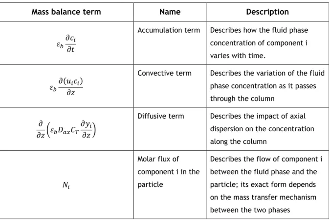
Table 3.1 – Meaning of the main terms present the in mass balance equations.

Mass balance term Name Description

𝜀_𝑏𝜕𝑐𝑖 𝜕𝑡

Accumulation term Describes how the fluid phase concentration of component i varies with time.

𝜀_𝑏𝜕(𝑢𝑖𝑐𝑖) 𝜕𝑧

Convective term Describes the variation of the fluid phase concentration as it passes through the column

𝜕

𝜕𝑧(𝜀𝑏𝐷𝑎𝑥𝐶𝑇 𝜕𝑦_𝑖

𝜕𝑧)

Diffusive term Describes the impact of axial dispersion on the concentration along the column

𝑁_𝑖

Molar flux of component i in the particle

Describes the flow of component i between the fluid phase and the particle; its exact form depends on the mass transfer mechanism between the two phases

The non-dimensional number that affects this equation is the Péclet number, defined by: 𝑃𝑒 = 𝑢𝐿

𝐷_𝑎𝑥 (3.26) where L is the column length. This number indicates how important the effects of axial dispersion are in the system.

(28)

Mathematical modelling 11 If there are no mass transfer resistances anywhere in the system, the molar flux of component i is given by equation (3.27). It adds a term representing the accumulation in the solid phase to the original equation.

𝑁_𝑖 = (1 − 𝜀_𝑏)𝜌_𝑝𝜕𝑞̅𝑖

𝜕𝑡 (3.27) where ρp is the particle porosity and 𝑞̅𝑖 the average concentration of component i in the

adsorbent particle. In this case, the component mass balance and the appropriate adsorption isotherm are enough to mathematically predict the breakthrough curves of the column. However, if mass transfer resistances are present in the micropores, an additional equation is required to describe intraparticular mass transfer. The LDF model was used and is given by equation (3.28). The employment of the LDF model allows for a much reduced computational time without losing accuracy in the solution.

𝜕𝑞̅_𝑖

𝜕𝑡 = 𝑘𝜇,𝑖(𝑞𝑠,𝑖− 𝑞̅𝑖) (3.28) where 𝑞𝑠,𝑖 the concentration of the component i at the surface of the adsorbent and 𝑘𝜇,𝑖 is the

micropore diffusion constant, given by equation (3.22).

The complexity of the model can be increased further if the resistance to the diffusion in the macropores is considered important. In a similar manner as before, a term representing the accumulation in the macropores must be added to the component mass balance as well as a new equation describing the diffusion in the macropores is necessary. The molar flux is now given by equation (3.29): 𝑁𝑖 = (1 − 𝜀𝑏) (𝜀𝑏 𝜕𝑐̅_𝑖 𝜕𝑡 + 𝜌𝑝 𝜕𝑞̅_𝑖 𝜕𝑡) (3.29) where 𝑐̅_𝑖 is the concentration of component i in the macropores. Equation (3.30) describes the diffusion in the macropores:

𝜕𝑐̅𝑖 𝜕𝑡 = 𝑘𝑝,𝑖 𝐵𝑖𝑖 𝐵𝑖_𝑖+ 1(𝑐𝑖− 𝑐̅𝑖) − 𝜌_𝑝 𝜀_𝑝 𝜕𝑞̅𝑖 𝜕𝑡 (3.30) where 𝑘_𝑝,𝑖 is the macropore diffusion constant and 𝐵𝑖_𝑖 is the mass Biot number. The macropore diffusion constant is given by:

𝑘_𝑝,𝑖 =15𝐷𝑝,𝑖

𝑟_𝑝2 (3.31)

where 𝐷_𝑝,𝑖 is the macropore diffusivity and 𝑟_𝑝 is the radius of the macropores. The mass Biot number is given by:

𝐵𝑖_𝑖 = 𝑟𝑝 𝑘𝑓,𝑖

(29)

Mathematical modelling 12 Finally, the diffusion in the film surrounding the pellet may be important as well. In that case, the molar flux assumes the form of equation (3.33):

𝑁_𝑖 = (1 − 𝜀_𝑏) 𝑎𝑝𝑘𝑓,𝑖

(𝐵𝑖 − 1)(𝑐𝑖− 𝑐̅𝑖) (3.33) where 𝑘_𝑓,𝑖 is the external mass transfer coefficient for i component.

In order to simulate breakthrough curves with n components, n component mass balance equations together with the respective mass transfer equations are required. The process can also be described with n – 1 mass balance equations and an overall mass balance, obtained by applying a sum over all n mixture components as presented in equation (3.34):

𝜀_𝑏𝜕𝐶𝑇 𝜕𝑡 = −𝑢𝑖𝜀𝑏 𝜕𝐶_𝑇 𝜕𝑧 − ∑ 𝑁𝑖 𝑛 𝑖=1 (3.34) where 𝐶_𝑇 is the total concentration in the fluid phase.

3.3.2 Momentum balance equation

The balance of forces acting over the characteristic control volume is described by the Ergun equation, which considers the change of velocity and pressure drop along the column. The Ergun equation is given by equation (3.35):

𝜕𝑃 𝜕𝑧 = − 150𝜇_𝑔(1 − 𝜀𝑏)2 𝜀_𝑏3_𝑑 𝑝2 𝑢_𝑖−1.75(1 − 𝜀𝑏)𝜌𝑔 𝜀_𝑏3_𝑑 𝑝 |𝑢𝑖|𝑢𝑖 (3.35) where 𝑃 is the total pressure, 𝜇_𝑔 is the gas viscosity and 𝜌_𝑔 is the gas density. Given that the gas phase is assumed to follow the ideal gas law, the total pressure in the system is related to the total concentration through the ideal gas equation:

𝑃𝑇 = 𝐶𝑇ℜ𝑇 (3.36)

However, the ideal gas equation is only accurate in the low pressure range. For the mixture studied in this work, the gas density has been shown to deviate from the ideal trend at pressures above 30 bar and therefore employing that equation can introduce significant errors [22]_{. The}

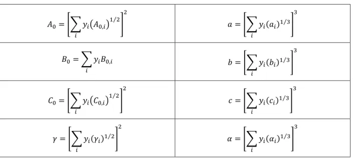
Benedict-Webb-Rubin (BWR) equation of state was used to relate the pressure in the system with the total concentration in the fixed bed experiments with pressures higher than 30 bar. 𝑃 = ℜ𝑇𝐶_𝑇+ (𝐵_𝑜ℜ𝑇 − 𝐴₀−𝐶0 𝑇2) 𝐶𝑇2+ (𝑏ℜ𝑇 − 𝑎)𝐶𝑇3+ 𝑎𝛼𝐶𝑇6+ 𝑐𝐶_𝑇3 𝑇2 (1 + 𝛾𝐶𝑇2)𝑒−𝛾𝐶𝑇 2 (3.37)

(30)

Mathematical modelling 13 Table 3.2 – Expressions used to calculate the mixing parameters of the BWR equation.

𝐴₀= [∑ 𝑦𝑖(𝐴0,𝑖)1 2 ⁄ 𝑖 ] 2 𝑎 = [∑ 𝑦𝑖(𝑎𝑖)1 3⁄ 𝑖 ] 3 𝐵₀ = ∑ 𝑦_𝑖𝐵_0,𝑖 𝑖 𝑏 = [∑ 𝑦𝑖(𝑏𝑖 )1 3⁄ 𝑖 ] 3 𝐶₀= [∑ 𝑦𝑖(𝐶0,𝑖)1 2 ⁄ 𝑖 ] 2 𝑐 = [∑ 𝑦𝑖(𝑐𝑖)1 3⁄ 𝑖 ] 3 𝛾 = [∑ 𝑦𝑖(𝛾𝑖)1 2⁄ 𝑖 ] 2 𝛼 = [∑ 𝑦𝑖(𝛼𝑖)1 3⁄ 𝑖 ] 3

Table 3.3 – Constants of the BWR equation for CH4 and CO2.

𝑎 𝐴₀ 𝑏 𝐵₀ 𝑐 𝐶₀ 𝛼 𝛾

CH4 5 187.91 3.38 × 10-3 4.26 × 10-2 2.58 × 105 2.29 × 106 1.24 × 10-4 6 × 10-3

CO2 13.86 277.30 7.21 × 10-3 4.99 × 10-3 1.51 × 106 1.40 × 107 8.47 × 10-5 5.4 × 10-3

3.3.3 Energy balance equations

Two different types of energy balance can be considered. If the three phases present in the column (gas, solid and column wall) are in thermal equilibrium (in other words, the heat transfer resistances are negligible between these three phases) then only one equation is necessary, named the “homogeneous energy balance”. If, on the other hand, the heat transfer resistances are important, each phase requires an independent energy balance that are then coupled to each other through film energy transfer terms. This model is called “heterogeneous energy balance”.

Heterogeneous energy balance

The gas phase energy balance is given by equation (3.38): 𝜀_𝑏𝐶_𝑇𝐶_𝑣,𝑖𝜕𝑇𝑔 𝜕𝑡 = 𝜕 𝜕𝑧(𝜆 𝜕𝑇_𝑔 𝜕𝑧) − 𝐶𝑇𝐶𝑝𝑔 𝜕(𝑢𝑖𝑇𝑔) 𝜕𝑧 + 𝜀𝑏ℜ𝑇𝑔 𝜕𝐶_𝑇 𝜕𝑡 − (1 − 𝜀𝑏)𝑎𝑝ℎ𝑓(𝑇𝑔− 𝑇𝑠) − 2ℎ_𝑤 𝑟_𝑤 (𝑇𝑔− 𝑇𝑤) (3.38) where 𝐶_𝑣,𝑖is the molar constant volumetric heat of component I, 𝜆 is the axial heat dispersion coefficient, 𝐶_𝑝𝑔 is the molar constant pressure specific heat of the gas mixture,

(31)

Mathematical modelling 14 ℜ is the ideal gas constant, ℎ_𝑓 is the film heat transfer coefficient between the gas and the solid phase, ℎ_𝑤 is the film heat transfer coefficient between the gas phase and the column wall, 𝑟_𝑤 is the radius of the wall, 𝑇_𝑔 is the temperature of the gas, 𝑇_𝑠 is the temperature of the solid and 𝑇_𝑤 is the temperature of the wall.

The energy balance in the solid phase is given by equation (3.39): (1 − 𝜀_𝑏) {𝜀_𝑝∑ 𝑐̅_𝑖𝐶_𝑣,𝑖+ 𝜌_𝑝𝜔_𝑐∑ 𝑞̅_𝑖𝐶_{𝑣,𝑎𝑑𝑠,𝑖}+ 𝜌_𝑝𝐶_𝑝𝑠 𝑛 𝑖=1 𝑛 𝑖=1 }𝜕𝑇𝑠 𝜕𝑡 = (1 − 𝜀_𝑏)𝜀_𝑝ℜ𝑇_𝑠𝜕𝑐̅ 𝜕𝑡+ 𝜌𝑏𝜔𝑐∑(−Δ𝐻𝑖) 𝜕𝑞̅_𝑖 𝜕𝑡 + (1 − 𝜀𝑏)𝑎𝑝ℎ𝑓(𝑇𝑔− 𝑇𝑠) 𝑛 𝑖=1 (3.39)

where 𝐶_{𝑣,𝑎𝑑𝑠,𝑖} is the molar constant volumetric specific heat of component i adsorbed, 𝐶_𝑝𝑠 is the constant pressure specific heat of the adsorbent and 𝜔𝑐 is the crystal weight fraction of the

pellet.

Finally, the column wall energy balance described by equation (3.40) completes the model.

𝜌_𝑤𝐶_𝑝𝑤𝜕𝑇𝑤

𝜕𝑡 = 𝛼𝑤ℎ𝑤(𝑇𝑔− 𝑇𝑤) − 𝛼𝑤𝑙𝑈(𝑇𝑤− 𝑇∞) (3.40) where 𝜌_𝑤 is the wall density, 𝐶_𝑝𝑤 is the specific heat of the adsorbent, 𝑈 is the global external heat transfer coefficient, 𝑇_∞ is the ambient temperature, 𝛼_𝑤 is the ratio of the internal surface area to the volume of the column wall, given by:

𝛼𝑤 =

𝑑_𝑤

𝑒(𝑑𝑤+ 𝑒) (3.41)

where 𝑑𝑤 is the column internal diameter and 𝑒 is the thickness of the shell and 𝛼𝑤𝑙 is the ratio

of the logarithmic mean surface area of the column shell to the volume of the column wall, given by:

𝛼_𝑤𝑙 = 1

(𝑑𝑤+ 𝑒) ln (𝑑𝑤_𝑑+ 𝑒

𝑤 )

(3.42)

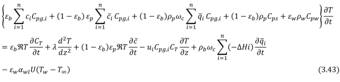
Homogeneous energy balance

The homogeneous energy balance allows for a shorter computational time without affecting accuracy, if the heat transfer resistances are negligible. This model combines the gas, solid and wall balances into equation (3.43):

(32)

Mathematical modelling 15 {𝜀𝑏∑ 𝑐𝑖𝐶𝑝𝑔,𝑖+ (1 − 𝜀𝑏) 𝑛 𝑖=1 𝜀_𝑝∑ 𝑐̅_𝑖 𝑛 𝑖=1 𝐶_{𝑝𝑔,𝑖}+ (1 − 𝜀_𝑏)𝜌𝑝𝜔𝑐∑ 𝑞̅𝑖 𝑛 𝑖=1 𝐶_{𝑝𝑔,𝑖}+ (1 − 𝜀_𝑏)𝜌𝑝𝐶𝑝𝑠+ 𝜀𝑤𝜌𝑤𝐶𝑝𝑤} 𝜕𝑇 𝜕𝑡 = 𝜀_𝑏ℜ𝑇𝜕𝐶𝑇 𝜕𝑡 + 𝜆 𝑑2_𝑇 𝑑𝑧2+ (1 − 𝜀𝑏)𝜀𝑝ℜ𝑇 𝜕𝑐̅ 𝜕𝑡− 𝑢𝑖𝐶𝑝𝑔,𝑖𝐶𝑇 𝜕𝑇 𝜕𝑧 + 𝜌𝑏𝜔𝑐∑(−∆𝐻𝑖) 𝜕𝑞̅𝑖 𝜕𝑡 𝑛 𝑖=1 − 𝜀𝑤𝛼𝑤𝑙𝑈(𝑇𝑤− 𝑇∞) (3.43)

where 𝜀_𝑤 is a geometric factor given by: 𝜀_𝑤=4(𝑑𝑤+ 𝑒)𝑒

𝑑_𝑤2 (3.44)

Since this model assumes thermal equilibrium between the different phases: 𝑇 = 𝑇_𝑔= 𝑇_𝑠= 𝑇_𝑤

The meaning of the main terms presented in these mathematical models is described in Table 3.4:

Table 3.4 – Meaning of the main terms present in the energy balance

Energy balance term Name Description

𝜀_𝑏𝐶_𝑇𝐶_𝑣,𝑖𝜕𝑇𝑔 𝜕𝑡

Fluid phase accumulation term

Describes stagnant fluid-phase energy accumulation over time.

𝐶𝑇𝐶𝑝𝑔𝜕(𝑢𝑖

𝑇𝑔)

𝜕𝑧

Convective term Describes the passage of energy through the column due to convection.

𝜕 𝜕𝑧(𝜆

𝜕𝑇_𝑔 𝜕𝑧)

Diffusive term Describes the transport of energy due to diffusion.

𝜌_𝑏𝜔_𝑐∑(−Δ𝐻_𝑖)𝜕𝑞̅𝑖 𝜕𝑡

𝑛 𝑖=1

Generation term Describes the generation of energy due to adsorption. (1 − 𝜀𝑏) {𝜀𝑝∑ 𝑐̅𝑖𝐶𝑣,𝑖 𝑛 𝑖=1 + 𝜌_𝑝𝜔_𝑐∑ 𝑞̅_𝑖𝐶_{𝑣,𝑎𝑑𝑠,𝑖}+ 𝜌_𝑝𝐶_𝑝𝑠 𝑛 𝑖=1 }𝜕𝑇𝑠 𝜕𝑡 Solid phase accumulation term

Describes the accumulation of energy in the solid phase over time.

(1 − 𝜀_𝑏)𝑎_𝑝ℎ_𝑓(𝑇_𝑔− 𝑇_𝑠) Gas-solid

exchange term

Describes how the fluid and solid phases exchange energy.

(33)

Mathematical modelling 16 2ℎ_𝑤

𝑟𝑤 (𝑇𝑔− 𝑇𝑤)

Gas-wall exchange term

Describes how the fluid phase and the column wall exchange energy.

𝛼_𝑤𝑙𝑈(𝑇_𝑤− 𝑇_∞)

Wall-Exterior exchange term

Describes how the column wall exchanges energy with the surrounding environment.

3.3.4 Transport parameters

The solution of the equations described above requires knowing the values of the various transport parameters that are present in them. These parameters were estimated with the correlations presented below.

The pore diffusivity, 𝐷𝑝,𝑖, was approximated using the Bosanquet relationship, presented

in equation (3.45): 1 𝐷_𝑝,𝑖 = 𝜏 ( 1 𝐷_𝑚,𝑖+ 1 𝐷_𝑘,𝑖) (3.45) where 𝜏 is the tortuosity factor, 𝐷_𝑚,𝑖 is the molecular diffusion coefficient for the component i in the mixture and 𝐷_𝑘,𝑖 is the Knudsen diffusion.

The molecular diffusivity is estimated with equation (3.46). 𝐷𝑚,𝑖 = 1 − 𝑦_𝑖 ∑ 𝑦𝑖 𝐷𝑖𝑗 𝑛 𝑗=1,𝑗≠𝑖 (3.46) where 𝐷𝑖𝑗 are the molecular diffusivities of the components in the mixture.

The Knudsen diffusivity is given by expression (3.47): 𝐷_𝑘,𝑖 = 9.7 × 10−9_𝑟

𝑝√

𝑇

𝑀𝑖 (3.47)

where 𝑟𝑝 is the pore radius in Å while the remaining variables are in SI units.

The axial dispersion parameters, 𝐷𝑎𝑥,𝑖 and 𝜆 were calculated with the following

correlations: 𝜀_𝑏𝐷_{𝑎𝑥,𝑖}

𝐷_𝑚,𝑖 = 20 + 0.5𝑆𝑐𝑖𝑅𝑒 (3.48) 𝜆

𝑘_𝑔= 7 + 0.5𝑃𝑟𝑅𝑒 (3.49) where 𝑆𝑐_𝑖 is the Schmidt number for component i, 𝑅𝑒 is the Reynolds particle number, 𝑃𝑟 is the Prandtl number and 𝑘_𝑔 is the thermal conductivity of the gas. These correlations are valid for values of the Reynolds number between 3 and 10000 with the dimensionless numbers involved being defined by the equations below:

(34)

Mathematical modelling 17 𝑆𝑐_𝑖 = 𝜇 𝜌𝐷_𝑚,𝑖 (3.50) 𝑅𝑒 =𝜌𝑢𝑑𝑝 𝜇 (3.51) 𝑃𝑟 =𝐶𝑝𝑔𝜇 𝑘_𝑔 (3.52) The molar specific heat at constant pressure is calculated as presented in the equation: 𝐶_𝑝𝑔= ∑ 𝑦_𝑖

𝑛 𝑖=1

𝐶_{𝑝𝑔,𝑖} (3.53) where 𝐶_{𝑝𝑔,𝑖} are calculated with the following polynomials:

𝐶_{𝑝𝑔,𝑖} = ∑ 𝐴_𝑖𝑇𝑖 3 𝑖=0

(3.54) where 𝐴𝑖 are empirical constants for each component and 𝑇 is the gas temperature. The molar

specific heat at constant volume of the mixture and those of each component were calculated from the respective specific heats at constant pressure according to the ideal gas relationships: 𝐶_{𝑣𝑔,𝑖} = 𝐶_{𝑝𝑔,𝑖}− ℜ

𝐶_𝑣𝑔= 𝐶_𝑝𝑔− ℜ

The gas thermal conductivity of a single component is calculated as follows: 𝑘𝑔,𝑖= (𝐶𝑝𝑔,𝑖+

5 4

ℜ

𝑀𝑖) 𝜇𝑖 (3.55)

and the one of the mixture with the following equation: 𝑘_𝑔= ∑ 𝑦𝑖𝑘𝑔,𝑖

∑𝑛𝑗=1𝑦𝑗Φ𝑖𝑗 𝑛

𝑖=1

(3.56) The film mass and heat transfer coefficients 𝑘_𝑓,𝑖 and ℎ_𝑓 were estimated using the following correlations: 𝑆ℎ𝑖 = 2.0 + 1.1𝑅𝑒0.6𝑆𝑐_𝑖 1 3 ⁄ (3.57) 𝑁𝑢 = 2.0 + 1.1𝑅𝑒0.6_𝑃𝑟1⁄₃_(3.58)

where 𝑆ℎ_𝑖 is the Sherwood number for component i and 𝑁𝑢 is the Nusselt number. These dimensionless numbers are calculated as follows:

𝑆ℎ_𝑖 =𝑘𝑓,𝑖𝑑𝑝

𝐷_𝑚,𝑖 (3.59) 𝑁𝑢 =ℎ𝑓𝑑𝑝

𝑘𝑔 (3.60)

The global heat transfer coefficient can be obtained from equation (3.61): 1 𝑈 = 1 ℎ_𝑤+ 𝑒𝑑𝑖𝑛 𝜆_𝑤𝑑_𝑙𝑛+ 𝑑𝑖𝑛 𝑑_𝑒𝑥ℎ_𝑒𝑥 (3.61)

(35)

Mathematical modelling 18 where 𝑒 is the wall thickness, 𝑑_𝑖𝑛 is the internal column diameter, 𝜆_𝑤 is the wall conductivity, 𝑑_𝑒𝑥 is the external column diameter, ℎ_𝑒𝑥 is the external convective heat coefficient, ℎ_𝑤 is the internal heat transfer coefficient and 𝑑_𝑙𝑛 is defined as follows:

𝑑𝑙𝑛=

(𝑑_𝑒𝑥− 𝑑_𝑖𝑛)

ln(𝑑𝑒𝑥⁄𝑑𝑖𝑛) (3.62)

The internal convective heat transfer coefficient between the gas and the wall column can be estimated with this correlation:

ℎ_𝑤𝑑_𝑖𝑛

𝑘𝑔 = 140 + 0.013396

𝑑_𝑖𝑛2

𝑑𝑝𝑘𝑔𝑅𝑒 (3.63)

3.3.5 Fixed bed initial and boundary conditions

The final element necessary to execute the simulations are the initial and boundary conditions of the model. In the fixed bed experiments, the column is initially filled with an inert gas, helium, and does not contain any other component. Additionally, the column should be regenerated, which means that the adsorbed concentration is zero. The temperatures in the fluid phase, solid and wall are all equal to the temperature of the inlet. Mathematically, this can be expressed with the equations below:

Initial conditions 𝑦𝑖 = 𝑞𝑖= 0 ∀ 𝑧, except for inert

𝑦𝑖𝑛𝑒𝑟𝑡 = 1 𝑇𝑔 = 𝑇𝑠= 𝑇𝑤= 𝑇𝑖𝑛𝑙𝑒𝑡 Boundary conditions Entering conditions, 𝑧 = 0 𝑢_{𝑖,𝑖𝑛𝑙𝑒𝑡}𝑐_{𝑖𝑛𝑙𝑒𝑡,𝑖} = 𝑢_𝑖𝑐_𝑖− 𝜀_𝑏𝐷_𝑎𝑥𝐶_𝑇𝜕𝑦𝑖 𝜕𝑧 𝑢_{𝑖,𝑖𝑛𝑙𝑒𝑡}𝐶_{𝑇,𝑖𝑛𝑙𝑒𝑡}𝐶_𝑝𝑇_{𝑖𝑛𝑙𝑒𝑡} = 𝑢_𝑖𝐶_𝑝𝑇_𝑔𝐶_𝑇− 𝜆𝜕𝑇𝑔 𝜕𝑧 𝑢𝑖,𝑖𝑛𝑙𝑒𝑡𝐶𝑇,𝑖𝑛𝑙𝑒𝑡= 𝑢𝑖𝐶𝑇 Exiting conditions, 𝑧 = 𝐿 𝜕𝑐_𝑖 𝜕𝑧 = 0 𝜕𝑇_𝑔 𝜕𝑧 = 0 𝑃 = 𝑃_𝑜𝑢𝑡

(36)

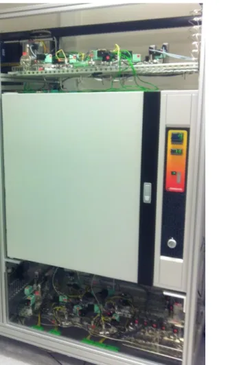
4 Experimental setup

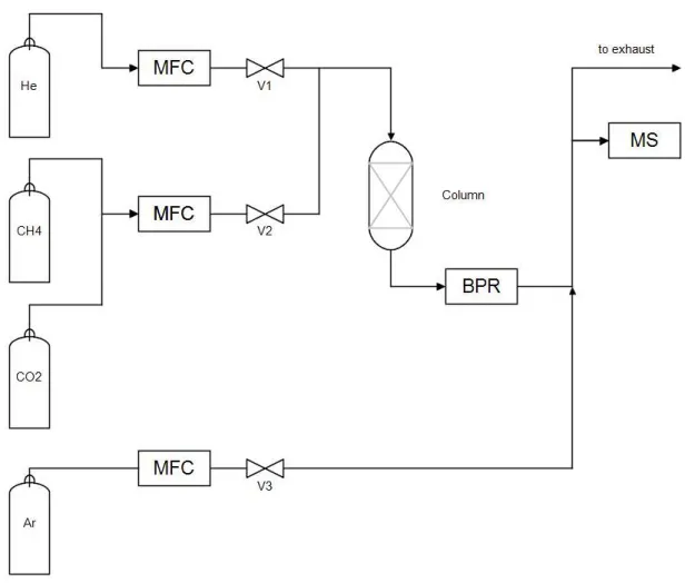
The fixed bed experiments were conducted in the PSA unit shown in Figure 4.1. A simplified scheme of the experimental setup is presented in Figure 4.2. This unit is generically composed of 4 columns and a set of different valves that allow the unit to run different regeneration cycles. Since the equipment was used to run breakthrough curve experiments, only one column was necessary. The unit was designed to run in a pressure interval of 0.1 – 70 bar and 298 – 550 K. The unit allows the connection of diverse analytical methods for analysis of the outlet components and includes an injection of a tracer gas (argon) to determine the existence of flow variations. For the CO2/CH4 separation, mass spectroscopy (MS) was the method used to

identify the composition of the outlet stream.

(37)

Mathematical modelling 20 Figure 4.2 – Simplified diagram of the experimental setup used for the breakthrough curve experiments. Abbreviations are as follows: MFC: mass flow controller, BPR: back-pressure regulator, MS: mass spectrometer.

The column is made of a steel tube 2.54 cm external diameter and 0.56 m long. The temperature changes inside the column were monitored by four thermocouples located at 0.05 m, 0.20 m, 0.35 m and 0.5 m from the feed inlet. These are located in the centre of the column. The device used for that purpose might affect the measurement of the last thermocouple, reducing the value.

The columns are located inside a ventilated oven. However, the ventilated air does not contact directly with the column. This means that while this is technically a case of forced convection, the overall heat transfer coefficient should not assume high values. In other words, it is rather a transition regime between forced and natural convection.

Table 4.1 summarizes the characteristics of the column, adsorbent and fixed bed experiments.

(38)

Mathematical modelling 21 Table 4.1 – Characteristics common to all fixed bed experiments

Packed column Length (m) 0.56 External diameter (m) 0.0254 Internal diameter (m) 0.0211 Bed voidage 0.377 Bed density (kg·m-3₎ ₆₆₀ Particle adsorbent Shape Cylindrical Mass (kg) 0.11789 Diameter (m) 9.0 × 10-4 Length (m) 1.8 × 10-3 Particle density (kg·m-3₎ ₁₀₆₀ Feed Temperature (K) 313.15 Composition 90 % CH4, 10 % CO2

Pressure (bar) From 5 to 70

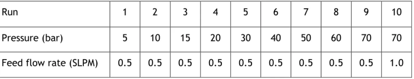
The breakthrough curves were measured at different inlet pressures, ranging from 5 to 70 bar. The experiment at 70 bar was carried out with two different feed flow rates. The differing features between the experiments are presented in Table 2.

Table 4.2 – Feed pressure and flow rates for the breakthrough curve experiments.

Run 1 2 3 4 5 6 7 8 9 10

Pressure (bar) 5 10 15 20 30 40 50 60 70 70

(39)

(40)

5 Results and Discussion

5.1 Adsorption equilibrium

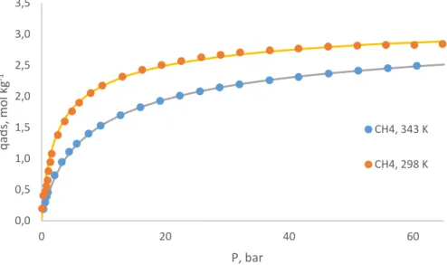
The adsorption equilibrium of CH4 was measured at 298 and 343 K in the pressure range of 0

to 65 bar. The isotherms are presented in Figure 5.1. The adsorption equilibrium of CO2 was

examined at the same temperatures and in the pressure range of 0 to 30 bar, with the results being presented in Figure 5.2. The measurements were made in a Belsorp Max Instrument.

Figure 5.1 – Adsorption isotherms of CH4. The points are the experimental data, the lines

represent the multisite Langmuir fit.

Figure 5.2 – Adsorption isotherms of CO2. The points are the experimental data, the lines

represent the multisite Langmuir fit.

0,0 0,5 1,0 1,5 2,0 2,5 3,0 3,5 0 20 40 60 q ad s, mol kg -1 P, bar CH4, 343 K CH4, 298 K 0,0 0,5 1,0 1,5 2,0 2,5 3,0 3,5 4,0 4,5 0 5 10 15 20 25 30 q ad s, mol kg -1 P, bar CO2, 343 K CO2, 298 K

(41)

Mathematical modelling 24 The feed stream in the breakthrough curve experiments will consist of 10 % CO2 and 90 %

CH4. The partial pressure of carbon dioxide will thus only go as high as 7 bar (for the 70 bar

experiment) while the methane partial pressure will reach 63 bar. The adsorption equilibrium of the two components was therefore studied in different pressure ranges.

In both cases, the experimental data was fitted with the multisite Langmuir isotherm. The CH4 data was fitted by minimizing the sum of the relative errors, while the CO2 parameters were

obtained by minimizing the sum of the relative and absolute errors. As explained in the section dedicated to the multisite Langmuir model, the product of the number of neighbouring sites occupied by a particle by the number of adsorption sites must remain constant for all thermodynamic consistency. To facilitate the optimization of the parameters, the CO2 data was

fitted first since it is usually harder to fit given the steepness of the isotherm. The CH4 isotherm

was then fitted with an added restriction so that the thermodynamic requirement was satisfied. The parameters were optimized with a code written in Python and are presented in Table 1.

Table 5.1 – Fitting parameters of the multisite Langmuir model.

qm / mol·kg-1 k0 / Pa-1 -ΔH / J·mol-1 a qm·a

CH4 3.493 8.169 × 10-10 21 410 2.047 7.151

CO2 4.299 8.436 × 10-10 23 201 1.663 7.151

The Python program uses the Nelder-Mead optimization method to determine the fitting parameters for different isotherms. The user can choose which isotherm model to use and which type of error to minimize. That information and the experimental data are read from a properly formatted excel file. The initial guess is written directly in the code. The program outputs a plot with the experimental data and the fitting model, the fitting parameters and the details of the optimization.

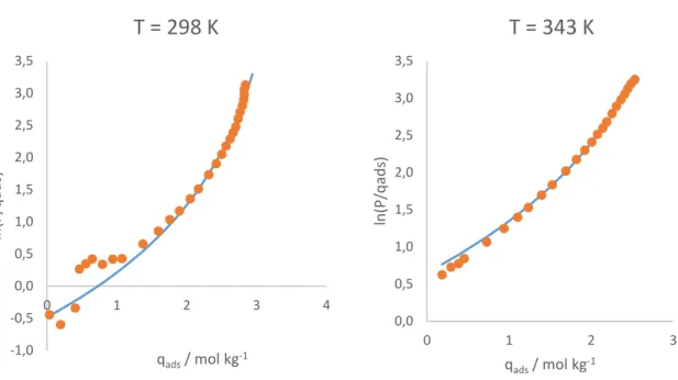
The quality of the experimental data and of the fitting model can be accessed by plotting the respective Virial curves. These consist in plotting the natural logarithm of 𝑃 𝑞⁄ _𝑎𝑑𝑠 as a function of the amount adsorbed, 𝑞_𝑎𝑑𝑠. For low values of adsorbent loading, the obtained graph should be linear, with the slope corresponding to the Henry constant of the component. This plot allows the removal outliers, which clearly stand out of the linear region of the graph. The Virial curves of the experimental data and of the fitting of the multisite Langmuir model are presented in Figures 5.3 and 5.4.

(42)

Mathematical modelling 25 Figure 5.3 – Virial plots for methane. Points are the experimental data and the solid lines

represent the multisite Langmuir fit.

Figure 5.4 – Virial plots for carbon dioxide. Points are the experimental data and the solid lines represent the multisite Langmuir fit.

From the analysis of the Virial plots it can be concluded that all cases are linear for low values of 𝑞_𝑎𝑑𝑠, except for the isotherm of methane at 298 K. However, the respective mathematical model does not appear to have been affected by this. A difference between the data and the model can be seen in the CO2 isotherms for low adsorbent loading. This is probably

due to the fact the carbon dioxide isotherm is quite steep in that region, making the

-1,0 -0,5 0,0 0,5 1,0 1,5 2,0 2,5 3,0 3,5 0 1 2 3 4 ln (P/q ad s) q_ads / mol kg-1

T = 298 K

0,0 0,5 1,0 1,5 2,0 2,5 3,0 3,5 0 1 2 3 ln (P/q ad s) q_ads / mol kg-1

T = 343 K

-2,5 -2,0 -1,5 -1,0 -0,5 0,0 0,5 1,0 1,5 2,0 2,5 0 1 2 3 4 5 ln (P/q ad s) qads / mol kg-1

T = 298 K

-1,0 -0,5 0,0 0,5 1,0 1,5 2,0 2,5 0 1 2 3 4 ln (P/q ad s) qads / mol kg-1

T = 343 K

(43)

Mathematical modelling 26 mathematical fitting more difficult. Overall, it can be concluded that a satisfactory fit was reached.

From the comparison of the experimental data with fitted curves, it can be concluded that an overall good fit was reached. Furthermore, the obtained parameters are within the expected values: the heats of adsorption for the two components are similar to those found elsewhere [23], [24], [25]_{and the value of the 𝑎 parameter is not too high (a value above 20 is rather}

unrealistic, and would suggest that the model is not appropriate)[15]_{. In fact, this parameter is}

directly related to the size of the particles, and should be in accordance with that property. From the analysis of the isotherms, it is clear that the adsorbent as a greater affinity towards CO2, given its higher saturation capacity and the greater steepness of the curve when

compared with the methane isotherm.

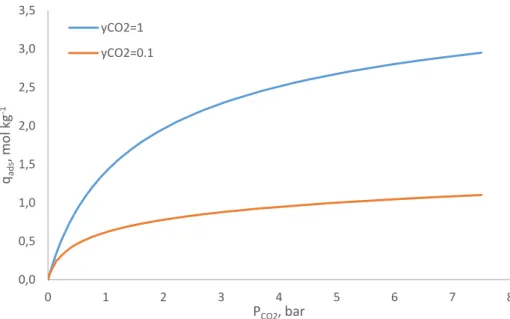
With the values of the isotherm parameters, it is possible to predict the shape of the multicomponent isotherms with the multicomponent extension presented in equation (3.6). Figures 3 and 4 present these curves at 313 K, for a system with 90 % methane and 10 % carbon dioxide, the same as the feed used in the fixed bed experiments.

Figure 5.5 – Carbon dioxide isotherms at 313 K: pure component and in a mixture with 90 % methane and 10 % carbon dioxide.

0,0 0,5 1,0 1,5 2,0 2,5 3,0 3,5 0 1 2 3 4 5 6 7 8 qad s , m o l k g -1 P_CO2, bar yCO2=1 yCO2=0.1

(44)

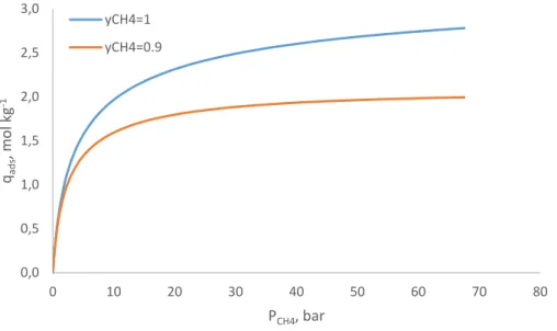
Mathematical modelling 27 Figure 5.6 – Methane isotherms at 313 K: pure component and in a mixture with 90 %

methane and 10 % carbon dioxide.

These curves are relevant when analysing the capacity exhibited by the adsorbent in the fixed bed experiments. It can also be concluded that the selectivity exhibited by the adsorbent is quite poor. That does not mean that it is not an effective adsorbent for this separation. If a component diffuses more rapidly through the pores, it will be preferentially adsorbed in the early stages of the process, regardless of the equilibrium state [26]_{. In other words, it is possible to}

achieve the separation if the kinetic selectivity is important.

5.2 Adsorption kinetics

The adsorption kinetics experiments were performed at low pressures, so it can be assumed that they operated in the linear zone of the isotherms. In addition, they can be considered isothermal. These conditions allow the use of the mathematical described in Chapter 3 to fit the experimental data.

The uptake curves were measured in a volumetric unit. Data was received every second for the first isotherm point. Equilibrium was assumed if the pressure variations were inferior to 1 × 10−3_{𝑘𝑃𝑎 for a period of 9999 seconds, the maximum allowed by the equipment.}

The results of the experiments described for the kinetics of CO2 and CH4 are presented in

Figure 5 and 6. In Figure 5, the curves are presented as a function of time, and clearly show that carbon dioxide diffuses through the micropores at a much faster rate than methane. Equilibrium is reached with CO2 after approximately 800 seconds (around 13 minutes), at a time when the

𝑞 𝑞⁄ _𝑒𝑞 factor for CH4 is only at 0.07. Equilibrium for methane is reached after over 90 000

seconds, which corresponds to 25 hours.

0,0 0,5 1,0 1,5 2,0 2,5 3,0 0 10 20 30 40 50 60 70 80 qad s , m o l k g -1 P_CH4, bar yCH4=1 yCH4=0.9

(45)

Mathematical modelling 28 Figure 5.7 – Adsorption kinetics of CO2 and CH4 at 298 K.

Figure 5.8 - Adsorption kinetics of CO2 and CH4 at 298 K against the square root of time.

The effect of the surface barrier at the mouth of the micropore is visualized by a small slope in the initial moments [25]_{. To enhance this effect, the same results were plotted over the}

square root of time, as presented in Figure 6. The slope is clearly visible in the methane curve, indicating that the constriction at the mouth of the micropore has an important contribution to the overall diffusion resistance. For carbon dioxide, however, this effect is not observed. This difference in the kinetic behaviour of the two components is expected, given that CO2 is the

smaller molecule of the two, with a kinetic diameter of 3.3 Å against 3.8 Å of methane. The parameters that affect the kinetics of methane were estimated using gPROMS with the model described in Chapter 3.2. Two different sets of parameters were considered, with the results being presented in Figure 5.9.

0,0 0,2 0,4 0,6 0,8 1,0 0 20000 40000 60000 80000 q qeq -1 t, s CH4 CO2 0,0 0,2 0,4 0,6 0,8 1,0 0 50 100 150 200 250 300 q qeq -1 t1/2_{, s}1/2 CH4 CO2

(46)

Mathematical modelling 29 Figure 5.9 - Adsorption kinetics of CH4 at 298 K with the solid lines representing the

mathematical models. The orange curve corresponds to 𝐷𝑐

𝑟𝑐2= 3.0 × 10 −6_𝑚2_𝑠−1_and_𝑘 𝑏 = 6.5 × 10−5𝑠−1. The grey curve corresponds to 𝐷𝑐 𝑟𝑐2= 1.2 × 10 −6_𝑚2_𝑠−1_and_𝑘

𝑏= 1.0 × 10−4𝑠−1. The difference between the

experimental data and the model may be due to the resistance not being completely controlled by the constriction at the pore mouth.

The same procedure was followed for CO2. The constriction at the pore mouth does not

play a part in the carbon dioxide diffusion, so 𝑘_𝑏 = 0. The grey line corresponds to 𝐷𝑐

𝑟_𝑐2= 1.0 ×

10−3_𝑚2_𝑠−1_{and the yellow line}𝐷𝑐

𝑟𝑐2= 7.48 × 10

−4_𝑚2_𝑠−1_.

Since the barrier mass transfer resistance term is only negligible for carbon dioxide, the kinetics of this component can be fitted with the simplified model presented in Chapter 3.2. The data was fitted by minimizing the square of residuals, in a program written in Python. The value obtained for the diffusion constant was: 𝐾_{𝜇,𝐶𝑂}₂= 1.695 × 10−4_𝑠−1_{(represented by the orange}

line). Considering equation (3.22), these values are in accordance with each other.

0,00 0,25 0,50 0,75 1,00 1,25 0 20000 40000 60000 80000 q qeq -1 t, s

(47)

Mathematical modelling 30 Figure 5.10 – Adsorption kinetics of CO2 at 298 K with the solid lines representing the

mathematical models.

The Python program developed for adsorption kinetics uses the Nelder-Mead optimization method to fit the experimental data of uptake curves and obtain the diffusion constant of the respective component. Before proceeding to the fitting of the experimental data, the roots of equation (3.24) are determined with Python’s fsolve function. In the same manner as for the isotherm program, data are read from an excel file while the initial guess for the roots and for the diffusion constant are written in the code. The program outputs a plot with the data and the fitting model, the value of the diffusion constant and the details of the optimization. In addition, the program also outputs the list of the roots of equation (3.24), for the user to check if they are valid. The roots of that equation are periodic, but solvers sometimes require a very precise initial guess to find all of them.

5.3 Fixed bed experiments

The first step in the analysis of the breakthrough curve results is the treatment of the MS data. The MS analysis is not made immediately after the column outlet, but instead after going through the back pressure regulator and being mixed with a constant stream of argon. In addition, the data is delivered in the form of intensity signals, which do not correspond directly to the molar fraction. In order to obtain the proper breakthrough curves, first it is necessary to “normalize” the signals, by multiplying them by an appropriate number so that the equilibrium value is the expected one. Afterwards, the concentration histories at the exit of the column are obtained by solving a mass balance involving the added argon stream.

-0,2 0 0,2 0,4 0,6 0,8 1 0,00 0,25 0,50 0,75 1,00 0 500 1000 1500 q qeq -1 t, s