Determination of the material/geometry of the section most adequate for a static loaded beam subjected to a combination of bending and torsion

Hugo Miguel Andrade Lopes Figueiredo da

Silva

Determination of the material/geometry of

the section most adequate for a static loaded

beam subjected to a combination of

bending and torsion

ABSTRACT

The Finite Element Method (FEM) is widely used to solve structural analysis problems. In this work, a novel Finite Element Model Updating methodology for static analysis is presented. The aim of the work is to improve the quality of the results using the Finite Element Updating techniques, by optimizing geometric parameters of the models and material properties in order to minimize deflection. Deflection can be minimized by increasing the Inertia moment of the section and/or Young modulus of the material. The Young modulus can be optimized by selecting an adequate material. In this work, material selection charts were used to determine the most reliable material. The selected material was then tested by tensile and extensometry tests to obtain Young modulus, Yield stress, and Poisson coefficient. The Inertia moment can be maximized by improving the geometry of the section, such as adding ribs or webs. A substantial improvement of the deflection can be achieved, but, in order to obtain the best results, optimization must be used. A MATLAB program was used to optimize the ANSYS models using a programming code. In order to know if the results are getting worse or better in relation to the previous iterations, an objective function was defined. The model is optimized when is not possible to further optimize the objective function.

RESUMO

O método dos elementos finitos (FEM) é amplamente utilizado para resolver problemas de análise estrutural estática. Neste trabalho é apresentada uma nova metodologia de melhoria de modelos de elementos finitos para análise estática. O objectivo do trabalho é melhorar a qualidade dos resultados utilizando as técnicas de melhoramento de elementos finitos, através da optimização de parâmetros geométricos dos modelos e propriedades do material, de modo a reduzir os deslocamentos. Os deslocamentos podem ser minimizados através do aumento do momento de Inércia da secção e/ou módulo de Young do material. O módulo de Young pode ser optimizado através da escolha de um material adequado. Neste trabalho foram usadas cartas de selecção de materiais para determinar o material mais adequado. Foram feitos ensaios de extensometria e de tracção ao material seleccionado para obter as propriedades relevantes do material: módulo de Young, tensão de Cedência e coeficiente de Poisson. O momento de inércia pode ser maximizado melhorando a geometria da secção com nervuras ou redes longitudinais. Uma melhoria substancial do deslocamento pode ser obtida, mas, de modo a obter os melhores resultados, tem de se usar optimização. O programa MATLAB foi utilizado para optimizar os modelos do ANSYS com um código de programação. De modo a saber se os resultados estão a melhorar ou a piorar em cada iteração, em relação às iterações anteriores, uma função objectivo foi definida. O modelo está optimizado quando não é possível optimizar mais a função objectivo.

KEYWORDS

FINITE ELEMENT METHOD

FINITE ELEMENT MODEL UPDATING OPTIMIZATION

STRUCTURAL STATIC ANALYSIS MATERIALS SELECTION

ACKNOWLEDGMENTS

This work was a real pleasure, because it is strongly multi-subject, it gave to me scientific knowledge in those subjects and it has practical applications.

I want to acknowledge:

-My scientific supervisor Professor José Filipe Meireles, for all the dedication, help, and time spent in the orientation of my work.

-My father David, my mother Cidália, my sister Mara, my godmother Sónia, and my friend Daniel Veiga, for the incredible support, encouragement, and belief in the conclusion of this work.

-Mr. Araújo, material tests laboratory technician, for all the dedication in the mechanical tests performed during this thesis.

INDEX

1.2 Aim of this work ... 4

1.3 State of the art ... 5

1.3.1 Rigidity and the Finite Element Method ... 5

1.3.2 About Optimization methods ... 8

1.4 Context and purpose of the work and structure of the thesis... 9

CHAPTER 2-RELATED THEORY ... 11

2.1 Introduction to Finite Element Method ... 13

2.2 About ANSYS ... 15

2.3 Bending and Torsion loading ... 15

2.3.1 Mechanical deflection ... 16

2.3.1.1Differential elastic curve ... 16

2.3.1.2 Torsion deflection ... 17

2.3.1.3 Total deflection ... 21

2.4 Stresses in torsion and bending loading ... 21

2.5 Rigidity indices of materials ... 22

2.6 Relation between structural rigidity and material properties ... 24

2.7 Mechanical tests ... 26

2.7.1 About tensile test ... 26

2.7.2 Elastic and Plastic domains ... 27

2.7.3 Relevant properties obtained from a tensile test ... 28

2.7.3.1 Modulus of Elasticity ... 28

2.7.3.2 Yield stress ... 28

2.7.3.3 Rupture stress ... 28

2.7.3.4 Elongation ... 28

2.7.3.5 Ultimate Tensile Strength ... 29

2.7.4 Determination of the Young modulus in tensile test ... 30

2.8 About MATLAB ... 31

CHAPTER 3-EXPERIMENTAL PROCEDURE ... 35

3.1 Materials selection ... 37

3.1.1 Initial selection ... 37

3.1.2 Intermediate material selection ... 39

3.1.3 Final material selection ... 40

3.1.4 About commercial dual phase steels (High strength steels) ... 41

3.1.4.1 Main characteristics ... 41

3.1.4.2 About DOCOL dual phase steels ... 42

3.2 Section Optimization ... 44

3.2.1 Section Optimization: Main purposes... 44

3.2.2 Section optimization: Longitudinal Webs ... 45

3.2.3 Section optimization: Ribbing ... 47

3.3 FEM and Optimization ... 50

3.3.1 Introduction ... 50

3.3.2 Finite Element Method experimental procedure ... 50

3.3.3 The FEM models ... 52

3.3.4 Optimization Model ... 54

3.3.5 The MATLAB program ... 55

3.3.6 ANSYS Input file structure ... 59

4.1 Numeric approximation- Comparison between numeric and analytic methods ... 63

4.1.1 About the model ... 63

4.1.2 Beam Deflection by the Analytic method ... 63

4.1.2.1 Bending ... 63

4.1.2.2 Torsion ... 64

4.1.2.3 Total deflection ... 66

4.1.3 Beam Deflection by the numeric method ... 66

4.1.4 Comparison of numeric and analytic methods ... 67

4.2 Mechanical Tests ... 69

4.2.1 Denomination of the tested specimens ... 70

4.2.1.1 Tensile test ... 70

4.2.1.2 Extensometry test ... 70

4.2.2 Tensile test experimental results ... 70

4.2.2.1 Stress-Strain and Stress-Extension charts ... 70

4.2.2.2 Determination of Young modulus in tensile test ... 70

4.2.2.3 Determination of Yield stress in tensile test ... 71

4.2.2.4 Determination of the Poisson coefficient, normal stress, and Young modulus in extensometry test ... 72

4.3 Variable analysis ... 72

4.3.1 Variable analysis of model 1- ribbed plate ... 74

4.3.2 Variable analysis of model 2- tubular beam ... 74

4.4 Optimization results ... 75

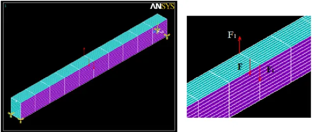
4.4.1 Model 1-Ribbed plate ... 75

4.4.1.1 Initial variable values and limits ... 75

4.4.1.2 Geometric parameters optimization results ... 76

4.4.1.3 Material properties optimization results ... 76

4.4.1.4 Optimization results using all variables ... 77

4.4.2 Model 2- Tubular beam ... 77

4.4.2.1 Initial variable values and limits ... 77

4.4.2.2 Geometric parameters optimization results ... 78

4.4.2.3 Material properties optimization results ... 79

4.4.2.4 Optimization results using all variables ... 79

4.5 Optimization settings ... 80

4.6 FEM results ... 81

4.6.1 Model1: Ribbed plate ... 81

4.6.1.1 Initial model results ... 81

4.6.1.2 Geometric parameters ANSYS results ... 81

4.6.1.3 Material properties ANSYS results ... 82

4.6.1.4 ANSYS results using all variables ... 83

4.6.2 Model2: Tubular beam ... 83

4.6.2.1 Initial model results ... 83

4.6.2.2 Geometric parameters ANSYS results ... 84

4.6.2.3 Material properties ANSYS results ... 85

4.6.2.4 ANSYS results using all variables ... 86

CHAPTER 5-RESULTS DISCUSSION AND CONCLUSIONS... 87

5.1 Results discussion ... 89

5.1.1 Variable analysis ... 89

5.1.1.1Material properties ... 89

5.1.1.2 Geometric parameters ... 89

5.1.1.2.1 Model 1: ribbed plate ... 89

5.1.1.2.2 Model 2: tubular beam ... 90

5.1.2 Mechanical tests ... 90

5.1.2.1 Extensometry test ... 90

5.1.2.2 Tensile test ... 90

5.1.4 FEM results ... 91

5.1.5 Materials selection ... 91

5.2 Conclusions of the work ... 92

5.3 Future work proposals ... 92

REFERENCES ... 95

Bibliographic references ... 97

ANNEXES ... 101

ANNEX 1-MECHANICAL TESTS ... 103

A1.0-Conditions of the Mechanical tests ... 105

A1.1-Stress-strain and stress-extension charts ... 105

Specimen 1 ... 105

Specimen 2 ... 106

A1.2-Determination of Young modulus in tensile test ... 107

Specimen 1 ... 107

Specimen 2 ... 108

A1.3-Charts used to determine Yield stress ... 108

Specimen 1 ... 108

Specimen 2 ... 109

A1.4-Determination of Poisson coefficient and Young modulus in extensometry test ... 109

ANNEX 2-VARIABLE ANALYSIS DATA ... 111

A2.1 Variable analysis data ... 113

A2.1.1 Model 1- Ribbed plate ... 113

A2.1.1.1 LG1 Variable ... 113

A2.1.1.2 LG2 Variable ... 114

A2.1.1.3 LG3 Variable ... 115

A2.1.1.4 EX Variable ... 116

A2.1.1.5 PXY Variable... 117

A2.1.1.6 DNS Variable ... 118

A2.1.2 Model 2- Tubular beam ... 119

A2.1.2.1 LG4 Variable ... 119

A2.1.2.2 LG5 Variable ... 120

A2.1.2.3 LG6 Variable ... 121

A2.1.2.4 EX Variable ... 122

A2.1.2.5 PXY Variable... 123

A2.1.2.6 DNS Variable ... 124

A2.2.1 Model 1: Ribbed plate ... 125 LG1 variable ... 125 LG2 variable ... 125 LG3 variable ... 126 EX variable ... 126 PXY variable ... 127 DNS variable ... 127

A2.2.2 Model 2: tubular beam ... 128

LG4 variable ... 128 LG5 variable ... 128 LG6 variable ... 129 EX variable ... 129 PXY variable ... 130 DNS variable ... 130

ANNEX 3-FINITE ELEMENT MODEL FILES ... 131

A3.1-Model 1: ribbed plate ... 133

A3.2-Model 2: Tubular beam ... 141

ANNEX 4-SCIENTIFIC PAPER ... 155

Abstract ... 157

1. Introduction ... 157

2. Bending and torsion combined load ... 158

3. The FEM models ... 159

4. Optimization Model ... 160

5. Materials selection ... 160

6 Results ... 161

6.1 Tensile test results ... 161

6.2 Extensometry test results ... 162

6.3 Optimization results ... 162

7. Results discussion and conclusions... 162

Nomenclature

Scalar

Symbol Units Description

a m/s2 Acceleration

as Scalar

as1 Scalar lower bound

as2 Scalar upper bound

A m2 Area of the cross section

Ai m2 Crosssectional area on the node i

Ai+1 m2 Crosssectional area on the node i+1

Am Coefficient matrix

A0 m2 Area of the mean line

ABS Absolute Value

b m Section width

b1 m Inner section width

bi m Distance between the binary forces

Bm Coefficient vector

c(xv) Function xv

C Pa.m Shear flux

C1,C2 Integration constants

D m Diagonal length of the initial beam section

e m Thickness

es Engineering strain

E GPa Young modulus

fd m Maximum deflection

f(as) Scalar function

f(x) Function f

F N Force

Fe N Force applied on each element

G GPa Transversal Elasticity Modulus

h m Section height

h1 m Inner section height

h(x) Function h

H Quadratic programming optimization Matrix

I m4 Axial Inertia moment

Ip m4 Polar inertia moment

k Element stiffness

K(xv,w) Function K

l m Element length

lb Lower Bound

lt m Mean line perimeter

L m Length

Li m Instantaneous length of the specimen on tensile test

m kg Mass

m1 kg Mass of the object 1

m2 kg Mass of the object 2

ma Lower limit or upper limit constraints

me Equality constraints mf Inequality constraints Mf(x) N.m Bending moment Mt N.m Torsion Moment n Safety coefficient q(x) m Objective function

r m Distance of the point to the action line of the force

s Slope of the recta

ub Upper bound

ui N Force on the elements at nodes i

ui+1 N Force on the elements at nodes i+1

V m3 Volume

w Weight of the optimization variables

x m x coordinate

x1 Optimization parameter 1

x2 Optimization parameter 2

xi m Nodal deflection on node i

xn Optimization parameter n

xv Vector of the optimization variables

y m y coordinate

y1 m Mean y coordinate of the object 1

y2 m Mean y coordinate of the object 2

yb m Deflection due to bending

ybc1 Boundary condition 1

ybc2 Boundary condition 2

yc m Centre of mass coordinate of the system

yt m Deflection due to torsion

ytotal m Deflection due to bending and torsion combined load

z m z coordinate

 Loading conditions coefficient

    ptimization parameter   g/m3 Density     Poisson coefficient     Unitary work     Rigidity coefficient

  degrees Diagonal angle of the initial beam  rad  Distortion angle

 Work produced by the relative displacement of the forces

    True strain

 Pa Shear stress

    Ratio of the rib height to the original height     Relative displacement

 Ratio of the rib width to the original profile width

  Pa Normal stress

b Pa Ultimate tensile strength

Symbol Description

0 Initial

1 First

avg Relative to average value

0.2 Relative to Yield

eq Relative to equivalent

flex Relative to flexure (bending)

gen Relative to generalized rigidity index

l Relative to the lower limit

long Relative to longitudinal direction

trans Relative to transversal direction

tens Relative to tensile

total Relative to torsion and bending combined load

tors Relative to torsion

T Relative to transverse matrix

u Relative to the upper limit

xx Relative to the x axis

y Relative to y direction

Operators

Symbol Description

ds Distance between two points

dx 1st order differential of x coordinate

dy 1st order differential of y coordinate

d2x 2th order differential of x coordinate

d2y 2th order differential of y coordinate

Abbreviations

Symbol Description

ASCII American Standard Code for Information Interchange

ANSYS Commercial Finite Element Method program

CFRP Carbon Fiber reinforced polymer

CLM Coupled Local Minimizers

Const Constant value

DOCOL Commercial dual phase steel designation

DOF Degrees of freedom

FEM Finite element method

FGFEM Fixed Grid Finite Element Method

GFRP Glass Fiber reinforced polymer

HCT Commercial dual phase steel designation

HMAWV Hybrid Model Aerial Working Vehicle

MATLAB MATrix Laboratory software

MGA Modeling to Generate Alternatives

PRDNS, DNS Density variable

PREX, EX Young modulus variable

PRPXY, PXY Poisson coefficient variable PRLG1,LG1 Geometric variable 1 PRLG2,LG2 Geometric variable 2 PRLG3,LG3 Geometric variable 3 PRLG4,LG4 Geometric variable 4 PRLG5,LG5 Geometric variable 5 PRLG6,LG6 Geometric variable 6 LG7 Geometric constant

SQP Sequential Quadratic Programming

UTS Ultimate tensile strength

2D Two dimensional

1.1 Motivation

The projects of industrial equipments have suffered severe changes, mainly because of the increasing accelerations caused by electrical motors. Those motors are able to cause movements with very high accelerations, sometimes going up to twelve times the acceleration of gravity. The improvement of the movement capability makes necessary an improvement on the resistance and rigidity of structures. The rigidity is one of the basic factors that determine the working capability of equipments, and it usually has a superior effect than resistance on the structure dimensioning. The deflection increase due to high accelerations can cause problems on the equipment regular behaviour before the lack of resistance is problematic. The lack of rigidity in structures causes an increase of friction and wear in the mobile parts, but the main problem are the exaggerated vibrations, which sometimes disturb the adequate operation. To improve rigidity it is necessary to increase the Young modulus of the material and/or the Inertia moment of the material section. The rigidity also depends of the geometrical characteristics, the length of the object and the type of load. In the other hand, it is possible that some composites, such as the glass fiber reinforcement polymer, even having a lower Young modulus than most metals, could have a good mechanical behaviour, as well. Due to the low density of those materials, one can strengthen the structure using more material, and therefore, improve the inertia moment, having a low weight object as a result. The only problem is the high cost of those materials, which are usually more expensive than any commercial steel. The present work focuses the optimization of relevant parameters in structural static analysis by the Finite Element Method. The tools used are the ANSYS program, used for Finite Element modelling and the MATLAB program, used to run and optimize ANSYS models, running a programming code written specifically for this purpose.

1.2 Aim of this work

The main aim of this work is the development and analysis of a Finite Element Model Updating application for structural static analysis to optimize the mechanical behavior of the models when subjected to static combined loads. To achieve the aim, one must optimize geometric parameters and material properties, with the goal of maximizing the rigidity and minimizing the object mass. Rigidity is very important in what relates to engineering parts, because it determines the work capability of engineering industrial equipments. As told before, the importance of rigidity can be higher than resistance in what relates to equipment reliability. To achieve this aim, one has to focus on two main factors: The Young modulus and the Inertia moment. The Young modulus is only dependent of the chosen material, and the Inertia moment is highly dependent on the section of the object. In the other hand, a low mass is good because two factors: the material cost and the admissible acceleration. According to Newton 2th law (eq.1):

F a= m (Eq. 1) where: a is the acceleration F is the applied force m is the mass

A lower mass can increase the admissible acceleration that is possible for a system, if the Force F is kept constant. This is important because of the increasing accelerations of new industrial equipments. In the other hand, a good mass position leads to a higher inertia moment. Rigidity is of special importance in machines performing accurate operations, such as metal cutting tools (example: Laser cutting), where the dimensional precision of the final product must be as higher as possible. Rigidity is also very important in some manufacturing machines, mainly those used commonly to manufacture transport vehicles, aircraft and rockets. Special attention is given to rigidity problems presenting high tensile strength or super-high tensile strength materials, where those materials may drastically increase deflections. In fact, there is the tendency of reducing the strength object thickness because the Yield stress is higher in high-strength steels than in regular steel. However, their Young modulus is similar, which

means that if the material enters the plastic domain, the deflections should be similar if the objects have the same dimensions. Therefore, if the thickness of a high-strength steel object is decreased, there might be a drastic increase of deflection in comparison to a similar object, made of regular steel but with a higher thickness [1]. The applications of this work are the transversal beams of some industrial equipments, such as laser cutting machines and plotters.

1.3 State of the art

1.3.1 Rigidity and the Finite Element Method

Rigidity can be defined as the capability of a mechanical system to deflect as less as possible when subjected to external loads. If the rigidity of a system is higher in comparison to other considering the same applied loads and the same material, the deflections are lower. There are equations to evaluate the rigidity of structural parts by means of a stiffness coefficient. The stiffness coefficient is the ratio between the load F applied to a system and the maximum deformation f that results from the application of the load. In the case of tension-compression of a beam with constant cross-section in the elastic domain, the stiffness coefficient complies with Hooke´s law:

tens F EA

λ = =

f L

(Eq. 2) where:

tens is the rigidity coefficient in tension-compression

E is the Elasticity Modulus of the material A is the area of cross section of the beam

L is the beam length measured along the action of the force F is the applied load

f is the maximum deflection

When a beam with constant cross-section is subjected to torsion, the stiffness coefficient is the ratio between the applied torque moment Mt and the twist angle (eq.3):

t p

tors M GI

λ = =

θ L

where:

tors is the rigidity coefficient in torsion

G is the Shear Modulus of the material

Ip is the polar moment of inertia of beam section

L is the beam length measured along the action of the force Mt is the torsion moment

is the distortion angle

In the case of bending of a beam with constant cross-section, the stiffness coefficient can be expressed by the eq. 4:

flex F ₃ αEI λ = = f L (Eq. 4) where:

flex is the rigidity coefficient in bending

I is the axial inertia moment of the beam´s section is a coefficient depending upon loading conditions f is the maximum deflection

As described, the rigidity of the constructions is governed by the factors:

-E in tension-compression and bending and G in torsion

-The moment of inertia I or Ip respectively in bending or torsion loading

-Linear dimensions of the deformed body L -Type of loading and type of supports

The elasticity is a very stable characteristic of the metals and depends uniquely of the density of the atomic crystalline lattice (the mean inter-atomic distance). However, with the development of composite materials, it has become possible to have multiple materials in one object only with the aim of obtaining an adjustable mean Young modulus. In these circumstances, this strategy can be considered, along with Inertia moment improvement, the best practical way of improving rigidity of a system. Particularly in thin walled structures, like plates and shells, the stability of the systems is very important. One strategy that can be used against the lack of stability is the reinforcement of easily deformable sections in the system by introducing stiffness limits

between the deforming section and the rigid units, and providing higher rigidity on connecting points. Together with the increase in external sizes and decrease of wall sections thickness it is necessary to increase rigidity in the transversal directions of acting bending forces and torsion moments in order to avoid losses of construction stability. Ribbing has wide application in improving rigidity, particularly in thin walled components. Strength may significantly increase when one increase the rib thickness, particularly at the critical regions. The influence of relative rib pitch and width of ribs upon the rigidity and strength of a part is not easily expressed in a generalized form. Because of this fact, an optimization process that can help the designer in the most adequate selection between the existing valid solutions is very interesting and useful. The use of numeric methods of calculus, such as the Finite Element Method (FEM), controlled by optimization processes, can be a precious help in these cases [1]. There are scientific works about the application of the Finite Element Method in structural static and dynamic analysis. Y. Liu and L. Gannon wrote a paper entitled “Finite element study of steel beams reinforced while under load”, consisting of reinforcing a w-Shape steel beam with welded plates while under load. The Finite Element Method was used for its modeling with the finality of investigate the effect of some parameters related to the process [2]. Other authors, as G. Falsone, G. Ferro, demonstrated that “An exact solution for the static and dynamic analysis of FE discretized uncertain structures” can be obtained. The work is about the probabilistic analysis of FE discretized uncertain linear structures in the static and dynamic structural analysis. The authors concluded that the corresponding relationships between the response and the reduced number of variables may be trivially deduced from the exact ones [3]. The Fixed Grid Finite Element Method (FGFEM) method has been recently used by F. Daneshmand and M. Kazemzadeh-Parsi to study the “Static and dynamic analysis of 2D and 3D elastic solids using the modified FGFEM”. In this work a modification of the FGFEM is presented and used for the static and dynamic analysis of 2D and 3D elastic solids. The accuracy and convergence of the proposed method was analyzed via some numeric examples and the results were compared with analytic and numeric solutions. The authors conclude that the results show good agreement with the analytic and numeric solutions [4]. The mechanical behavior of shells of revolution was studied in the work “Nonlinear static and dynamic analysis of shells of revolution”, by C. Polat , Y. Calayir. In this work, geometrically nonlinear static and dynamic response of shells of revolution is investigated. During this work, a MATLAB code was developed to study geometrically

linear and nonlinear static and dynamic responses of shells of revolution. The authors conclude that the nonlinearity affect the solutions significantly [5].

1.3.2 About Optimization methods

B. Zárate and J. Caicedo studied multiple alternatives to the Finite Element Model Updating technique in the work “Finite element model updating: Multiple alternatives”. The authors studied a Finite Element Model Updating methodology of complex structural systems. Traditional Finite Element Model Updating techniques optimize an objective function to calculate one single optimal model that behaves similarly to the real structure and represents the physical characteristics of the structure. The author have discovered that a local minimum, rather than the global minimum could be a better representation of the physical properties of the structure, mainly due to numeric and identification errors, as well as the limited number of sensors in structures. The proposed method is based on MGA – Modeling to Generate Alternatives [6]. An optimization method called “Coupled Local Minimizers” was used by P. Bakir, E. Reynders, G. Roeck in the paper entitled “An improved Finite Element Model Updating method by the global optimization technique ‘Coupled Local Minimizers’ “.In this scientific work, a global optimization method called ‘Coupled Local Minimizers’ (CLM) is used for updating the Finite Element Model of a complex structure. The CLM method is compared with other local optimization methods such as the Levenberg– Marquardt algorithm, Sequential Quadratic Programming and Gauss–Newton methods and the results show that the CLM algorithm gives better results in Finite Element Model Updating problems compared to the above-mentioned local optimization methods [7]. The paper “Discrete optimization problems of the steel bar structures”, by S. Kalanta, J. Atkociunas, A. Venskus focus the optimal design problems of elastic and elastic-plastic bar structures. These problems are formulated as nonlinear discrete optimization. The main conclusions were: Elastic-plastic framed structure analysis confirmed the statement that often an optimal structure project is determined not by the strength, but the stiffness, stability and structural requirements, and, mathematical models and solution algorithms for 2D optimization problems can be adopted for solutions of 3D optimization problems [8]. X. Bin, C. Nan and C. Haunt have implemented “An integrated method of multi-objective optimization for complex mechanical structure”, where the authors present an integrated method of

multi-objective optimization for complex mechanical structures. It integrates prototype modeling, FEM analysis and optimization. To explore its advantages over traditional methods, optimization of a manipulator in hybrid mode aerial working vehicle (HMAWV) is adopted. The results indicated that this integrated method is effective and shows a potential in engineering applications. The authors concluded that this integrated method of multi-objective optimization has solved a practical problem successfully, and its efficiency has been improved greatly compared with enumerative methods [9]. Based on the work of this thesis, a scientific paper was written and oral presented on VI International Materials Symposium MATERIAIS 2011, held in University of Minho, Guimarães (Annex 4) [10].

1.4 Context and purpose of the work and structure of

the thesis

The most important goal of this work is the minimization of nodal deflections due to applied loads. Ribbing is an effective way of maximizing inertia moment. Therefore, there is the need of optimizing ribbing-related variables, such as rib thickness, length between consecutive ribs, and rib height, in the particular case of plate objects. When those three parameters are optimized using a suitable objective function, one can achieve good results. In the case of the tubular beam considered in this work, the relevant variables are: distance from the center to the corner segment in each side; length of the center segment, and height of the center segment. In the other hand, material properties, such as Young modulus and Poisson coefficient also affect the deflection results. Having this fact in consideration, all the variables were studied alone, in order to know how its variation affects the value of the objective function. In chapter 1, the state of the art is presented, as well as the motivation and the aim of this work. In chapter 2, the related theory is presented, including theory about mechanical tests, equation demonstrations and optimization. In Chapter 3, the experimental procedure is presented. This chapter is about the materials selection, section optimization, FEM models and the MATLAB optimization program. The results are presented on chapter 4. The chapter 4 is about mechanical tests results (tensile test and extensometry test), variable analysis of the two finite element models (ribbed plate and tubular beam), FEM results on ANSYS, and MATLAB optimization results (final values of the objective

function and variables). The optimization variables were six, in both models: three variables are geometric, and three variables are material properties. The geometric parameters are different in the two FEM models. However, the studied material properties are the same for the two models. Chapter 5 is about the results discussion and conclusions. It features mechanical tests, FEM, and optimization results discussion and conclusions. The Annex 1 contains the tensile test and extensometry test charts, featuring stress-strain charts, stress-extension charts, and charts used to determine two mechanical properties of the material: Yield stress and Young modulus. In the Annex 1, there are also the tables used to calculate Young modulus and Poisson coefficient in extensometry test. In the Annex 2, one can see the variable analysis data, featuring nodal deflection values and the charts obtained in the variable analysis. In the Annex 3 one can see the Finite Element Model input files, used to optimize the models on MATLAB. In the Annex 4 there is the scientific paper published during this thesis.

2.1 Introduction to Finite Element Method

The Finite Element Method is a numeric procedure that can be used to obtain solutions to a large number of engineering problems involving stress, deflection, heat transfer and electromagnetic phenomena. The finite element method (FEM) consists in a computer model that is analyzed under certain conditions. FEM is used either in new product design, and existing product refinement. It is very useful to verify if a proposed design will be able to perform to the client's specifications before manufacturing. A modification in an existing product or structure is usually done with the purpose of qualify the product or structure for a new service condition. In case of structural failure, FEM may be used to help the design improvement in order to meet the new service condition [11]. In the case of structural static analysis, which is the subject of this work, the model is statically loaded. In this work, one is analyzing the elastic domain only, due to the nature of the application. In the elastic domain, there is a linear relation between stress and strain. The proportionality constant is the Young modulus E, as shown next in eq. 5:

0

ΔL σ=Εε=E

L (Eq. 5)

where:

is theNormal stress is the Strain

is the Young modulus L is the length variation

L0 is the initial length of the object

In FEM, it is very important to assume a solution that approximates the behaviour of the elements. Considering the deflection of a solid member with a uniform cross-section A, a length L when subjected to a tensile Force F, one can say that the normal stress is given by eq. 6:

F σ=

where:

F is the applied force

A is the area of the cross-section

Using Eq. 5 and 6, one can obtain a new equation (Eq.7):

0

AE

F= ΔL

L (Eq. 7)

The elastic behaviour of an element can be modelled by an equivalent linear spring according to the eq. 8 [12]:

avg i+1 i

e eq i+1 i A E i+1 i (A +A )E i+1 i

F =k (u -u )= (u -u )= (u -u )

l 2l (Eq. 8)

where:

Fe is the force on the elements

Ai and Ai+1 are the cross sectional areas of the member at nodes i and i+1

Aavg is the average area

l is the length of the element

ui and ui+1 are the forces on the elements at nodes i and i+1, respectively

The equivalent element stiffness is k =eq (A +A )Ei+1 i

2l

Despite the advantages of the FEM, it has limitations that can lead to errors in the analysis results. In many practical engineering problems one cannot obtain exact solutions. The difficulties to obtain exact solutions may be attributed to either the complex nature of the governing differential equations or the difficulties that arise from dealing with the boundary and initial conditions. The errors that contribute to the models limitations can be divided into: User errors, due to mistakes in the data input process, such as physical properties and dimensions, misuse of the selected elements, misapplication of DOF constraints, low discretization of the geometry of the structure, for example, due to an inappropriate rough mesh size or an inaccurate approximation of geometries and inherent numeric methods errors used to solve the equilibrium equations. These errors are due to the finite precision of the method, where conditions are not controllable, or expected. For complex structures, even when using correct meshes for each specific problem, errors can be substantial. These errors occur due to difficulties in adapting the meshes to the geometry of the model [13].

2.2 About ANSYS

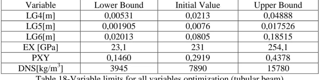
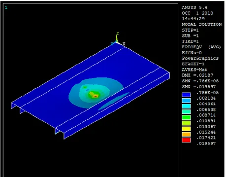
The implementation of the Finite Element Method usually follows three steps: Pre-processing, solution and post-processing. Within these three basic steps, there are sub- steps. In pre-processing, one defines the geometric model and builds the mesh with the elements. In this work, the sequence of creating the geometric model was: keypoints, then lines by keypoints and then areas by lines. The mesh makes possible the discretization of the elements on the domain, by assigning to each element segment a partial differential equation. All the differential equations are discretized after integration in the area of the elements. The equations are then solved by algebraic methods, such as gauss elimination method. In the solution menu it’s necessary to define the loads and the DOF displacements (constraints). After solving the model, the results can be viewed in the post-processing menu. For structural static analysis, as in this work, the most important are the stresses and the deflections. This work has the aim of obtaining the lowest possible deflections. Because of that, the results taken from the program were the deflections. The stresses are also an indicator of the mechanical behavior, since they are responsible for mechanical deflection. With FEM commercial software, such as ANSYS, all these steps can be performed through graphical interfaces or by command input.

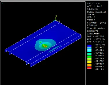
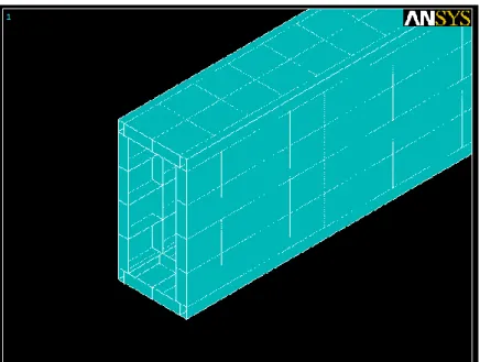
2.3 Bending and Torsion loading

In practice is very common to find situations where the objects are loaded with a combination of bending and torsion. Bending is usually due to central transverse load, and torsion can be due to transverse load that is not centered. In some situations, these two types of loading act at the same time, and so, one have a combination of bending and torsion. In bending there are only normal stresses, and in torsion there are only shear stresses. The next figure (fig. 1) shows the FEM model, its loading and DOF constraints used in the preliminary analysis. The considered load was a centred bending load F of 3528 N, which is 12 times the acceleration of gravity on a mass of 30 kg (12*9,8*30=3528 N) and a binary load Mt=0,2*F1 that produces torsion, in which F1 is

Fig. 1-Load applied to FEM models and DOF constrains

In torsion and bending combined loading, there are both shear stresses due to torsion and normal stresses due to bending. The total deflection is the sum of the deflection due to bending and the deflection due to torsion.

2.3.1 Mechanical deflection

2.3.1.1Differential elastic curve

The initial equation is:

f

1 M (x)

=

ρ EI (Eq. 9)

where:

1/is the inverse of the curvature radius Mf(x) is the applied bending moment

An approximation can be used to obtain a term which is a function of

2 2 d y dx : 2 2 2 3 2 2 ₂ d y 1 _dx d y ρ dx dy 1+ dx    _{ }   _ _      (Eq. 10)

Substituting and integrating:

2 f 2 1 d y EI =EI =M (x) ρ dx

x f 1 0 dy EIθ EI M (x)dx+C dx  



 

 

Constants can be determined by applying boundary conditions. For a simply supported beam, one has:

bc1 bc2

y =0,y =0

The final equation used to obtain the deflection is:

3 2 3 b 2 3 FL x x y = 3 -4 48EI L L       (Eq. 11) where:

yb is the deflection due to bending

F is the applied load

L is the length of the object x is the x coordinate

One can see that the deflection is dependent of both the geometry of the object (Inertia moment I and length L) and the material (Young modulus E). The deflection is also dependent on the load F and is a function of the x coordinate [14].

2.3.1.2 Torsion deflection

As a simplification, one can admit that the shear stress is constant along the thickness, with a better accuracy the thinner the object is in relation to the dimensions of the section. One can then demonstrate that the shear flux C=τt is constant, meaning that the shear stress is constant if the thickness is constant.

If e,e1 are the thicknesses, and ,are the shear stresses in any two points m and n, it is

possible to know, by sectioning n and m, that those sections are subjected to shear stresses equal to and The next figure (fig. 2 ) shows an illustration of a hollow-box

object, along with the representation of the shear stresses ,, the points m, n, the thicknesses e, e1 and the distance between two points ds.

Fig. 2-Representation of a hollow-box object and relevant torsion parameters [15]

Considering two points located on the object wall, separated by a distanceds, the flux is the same for the two points:

1 1

C=τe=τ e (Eq. 12)

where:

C is the shear flux is the shear stress e is the object thickness

A face eds is subjected to a forceτeds, and the moment of this force in relation to any point of the section is τerds, where r is the distance of the considered point to the action line of the force τeds. Considering that the sum of the moments in every point of the wall should be equal to the torsion moment:

τerds=Mt



Therefore, the flux

τe

t

τe rds=M



The above equation (Eq. 14) represents the double of the area A0 of the inner side of the

mean line. Solving the integral, one can find the expression of the shear stress due to torsion: t 0 M τ= 2A e (Eq. 15)

where:

is the shear stress Mt is the torsion moment A0 is the area of the mean line

e is the thickness

The unitary angle of torsion can be obtained by the laws of energy conservation, by considering equal the work of deformation of a beam part with unitary length to the inner work of the same part:

t

M θ ξ=

2 (Eq. 16)

where:

is the unitary work Mt is the torsion moment

is the twist angle due to torsion

The forces τeds applied to the horizontal faces of the volume element suffer the relative displacement . The work produced by them is:

1

= τeμds

2

 . (Eq. 17 )

where:

is the work produced by the relative displacement of the applied forces is the shear stress

e is the thickness

is the relative displacement

ds is the distance between the points n and m

Because the shear flux e on the vertical faces of the element moves perpendicularly to it, the work produced by them is null. The inner work of the entire object is then:

2

1 1 τ

ξ1= τeμds= eds

2





2 2 t ₂ t t 2 2 2 0 0 M θ 1 1 M M ds = τ eds= eds= 2 2G







The distortion angle is then: t 2 0 M ds θ= 4GA



If the thickness is constant, then the equation 18, reduces to:

t t t

2

0 0

M l Cl

θ= =

4GA e 2GA e (Eq. 19)

where:

is the twist angle C is the shear flux

lt is the mean line perimeter

G is the transversal elasticity modulus A0 is the mean line area

e is the object thickness Mt is the torsion moment

The deflection due to torsion can then be calculated [15]: t D

y = θL

2 (Eq. 20)

where:

yt is the deflection due to bending

D is the diagonal length of the object L is the length

 is the distortion angle

In the next figure (fig. 3), one can see an illustration of a hollow-box object subjected to torsion:

The fig. 3 shows the physical meaning of the torsion deflection yt, twist angle , and

half of the diagonal lengh D/2. 2.3.1.3 Total deflection

The total deflection can be expressed as the sum of the contributions of bending and torsion:

total b t

y

=y +y

where:

ytotal is the deflection due to bending and torsion combined load

yb is the deflection due to bending

yt is the deflection due to torsion

In a bending and torsion combined load, the resulting stresses are the combination of the normal stresses due to bending and the shear stresses due to torsion.

2.4 Stresses in torsion and bending loading

This work focuses the deflection dimensioning. There is another possible dimensioning approach: the stress dimensioning, which is based on stress criteria. The most common criteria are the Von Mises criterion and the Tresca criterion. To determine the admissible stress for a system, it is necessary to determine the main stresses after obtaining the normal stress due to bending and shear stress due to torsion. The normal stress due to bending can be calculated by:

f M y σ=± I (Eq. 22) where:

is the normal stress Mf is the bending moment y is the y coordinate

The shear stresses due to torsion in thin walled objects can be calculated by: t 0 M τ= 2tA



 is the shear stress due to torsion Mt is the torsion moment (torque)

t is the beam thickness

A0 is the section mean line area

After obtaining the admissible stress by the chosen criteria, one must chose a material with a Yield stress higher than the admissible stress as many times as the safety coefficient n value.

2.5 Rigidity indices of materials

It is possible to obtain a generalized strength-rigidity index, by using the factors that represent the weight advantage in terms of strength: σ0.2

γ and rigidity advantage: E

γ .

The generalized index is:

0.2 gen σ E λ = γ (Eq. 23) where:

gen is the generalized rigidity index

0.2 is the yield stress

E is the Young modulus is the density

This index represents the capability of a material to have the less deflection possible, and less weight when subjected to high loads. The fig. 4 shows the value of the generalized rigidity index for the most common engineering materials. The correspondence of the material to the number is as follows:

Fig. 4-Generalized strength-rigidity indices [1] According to the fig. 4, the materials can be separated in four groups: 1-Super high-strength steels ( gen8*105)

2-Alloy steels, titanium alloys and sitalls( 3,5*105





3-Carbon steels, high strength cast irons and wrought aluminium alloys ( gen1*105) 4-Structural bronzes, wrought magnesium alloys, cast aluminium alloys, cast magnesium alloys, grey cast irons ( gen0,5*105)).

In the table 1 one can see some properties of the most common structural materials, along with their rigidity characteristics. The material with highest generalized rigidity index is the high-strength steel, with a value of 8,4. The alloy steels are the second best, but are much worse than the first, with a value of 3,8. Titanium alloys and Sitalls have a value of 3,6, a value close to the alloy steels. The other materials have an index much lower than titanium alloys. For some materials, the index is slightly higher than 1, but for some materials it is substantially lower than one.

Materials Density (kgf/dm3 ) Modulus of elasticity (kgf/mm2) Rigidity characteristi c -3 b E *10 σ Generalized factor 0.2 _-5 σ Ε *10 γ Carbon Steels 7,85 21000 2,6 1,3 Alloy Steels 1,17 3,8 High-strenght Steels 0,6 8,4

Grey cast irons 7,2 8000 2,3 0,3

High-Strenght cast irons 7,4 15000 1,9 1,1

Aluminium alloys Cast 2,8 7200 2,9 0,45 Wrought 1,2 1,1 Magnesium alloys Cast 1,8 4500 2,1 0,32 Wrought 1,4 0,52 Structural Bronzes 8,8 11000 1,85 0,6 Titanium alloys 4,5 12000 0,8 3,6 Structural plastics Delta-wood 1,4 4000 2 - Glass-fibers 1,6 5000 1,67 - GFAM 1,9 6000 0,86 - Sitalls 3 15000 1,87 3,6

Table 1-Strenght and rigidity characteristics of structural materials [1]

The material selection for a structural application is determined by the strength-rigidity characteristics, but also by the relevant material properties for the considered application. The mechanical design has a very high importance, because it´s possible to build an object with high rigidity and strength, even when the material is not so stiff and strong. The shape is therefore more relevant than the material for the mechanical deflections reduction [1].

2.6 Relation between structural rigidity and material

properties

The rigidity of the structures is determined by the deflection. The deflection is dependent of the material properties and depends also of the geometric characteristics of the object. The bending deflection due to transverse load can be expressed, as told before, by: 3 2 3 b 2 3 FL x x y = 3 -4 48EI L L       (Eq. 11) where:

yb is the deflection (function of x coordinate)

I is the axial inertia moment of the section E is the Young modulus of the material L is the beams length

F is the applied load x is the x coordinate

One can see that the material selection plays an important role in this work, since there is a dependency of Young modulus on the deflection results. The results may vary drastically if a different material is used, mainly in terms of the Young modulus. The density is very important because the object mass is directly related to it:

m γ=

V (Eq. 24)

where:

is the density of the material m is the material mass

V is the object volume

As Newton´s second law say that:

F a=

m (Eq. 1)

where:

m is the mass of the material a is the acceleration

F is the applied force

One can see that a lower mass can be important to obtain a good behavior of the structure, since for a certain load, the lower the mass, the higher can be the acceleration

without structural failure, or/and undesirable vibrations. The density should be as low as possible because for an object of the same dimensions, the mass is lower the lower is the density. Two methodologies can be used in this work to achieve the goal of deflection minimization:

- The Young modulus of the material must be the highest possible, because the deflections are a function of it. This methodology is based on the importance of the material properties. The high-strength steels, such as dual-phase steels, seem to be the most suitable materials. This was the methodology used in this work.

- One can choose a material with not so high Young modulus, but with a relatively low density and low/medium cost that allows the maximization of the Inertia moment by means of object reinforcement with longitudinal webs or ribs. This methodology is based on the improvement of the Inertia moment. Some suitable materials for this methodology include composites, such as GFRP- Glass fiber reinforced polymer.

2.7 Mechanical tests

2.7.1 About tensile test

A tensile test, also known as tension test, is the most relevant type of mechanical test that can be performed on a material. It is used to determine the mechanical properties of metals and metallic alloys. The main advantages of tensile tests are: simplicity, they are relatively inexpensive, and fully standardized. As the test is performed, one will obtain a stress-strain curve similar to what is shown next: (fig. 5)

By performing this test, one can determine how the material reacts to the force being applied, and consequently, one is able to obtain the material´s most important properties, such as Young modulus, elongation, Yield stress, stress at rupture, elongation until fracture (%), and area reduction until fracture (%). The results obtained from the test can be used to build a normal strain chart and a normal stress-extension chart. The test specimens can be round, having 12,7 mm of diameter or can be flat. When the original material has enough thickness, the specimens are usually round. The reference length in the center of the specimen is usually 51 mm [17]. In the fig. 6 one can see a tensile test machine.

Fig. 6-Tensile test device [18]

2.7.2 Elastic and Plastic domains

The stress-strain chart shown on fig. 5 can be divided in two mechanical behavior domains. The elastic domain, used to estimate the Young modulus using Hooke’s law, and the plastic domain. In graphical terms, the elastic domain is the linear part of the graphic, where the stress is directly proportional to the strain, being the Young modulus the proportionality constant. The plastic domain is represented by a non-linear curve. The difference between the elastic and plastic domains is that when a load is applied and the material doesn´t leave the elastic domain, if the load is removed, then there will be no residual strain and the material returns to its original dimensions. If the plastic domain is reached, then there will be a residual strain after the load is removed, that will be higher the higher is the applied load when the load is removed. In the elastic domain, the Young modulus can be determined by the slope of the stress-strain curve [17].

2.7.3 Relevant properties obtained from a tensile test

2.7.3.1 Modulus of Elasticity

The modulus of elasticity is a measure of the stiffness of the material, but its determination is only valid in the linear region of the stress-strain chart. Even in the linear region of the chart, one cannot obtain the exact Young modulus, but an approximation. The Young modulus is constant in every point of the linear region of the stress-strain chart (elastic domain) [17].

2.7.3.2 Yield stress

The Yield stress of a material can be defined as the stress applied to the material at which plastic deformation starts to be relevant when the material is loaded. Because there is not a well defined point that is the end of the elastic domain region and the beginning of the plastic domain, one usually chooses a Yield stress for a certain plastic deformation. For structure projects, yield stress is usually calculated for a plastic deformation of 0,002, which is 0,2%. Yield stress is usually calculated by making a line, starting on the point 0,002 in the strain axis and stress equal to 0. The line is parallel to the elastic domain curve. The point where the recta intersects the plastic domain of the stress-strain curve is the Yield stress (stress axis) and Yield strain (strain axis) [17]. 2.7.3.3 Rupture stress

Rupture stress is the current stress when the specimen suffers rupture. In projects with ductile metallic alloys, the rupture stress is usually not an important value, because the correspondent strain is very high. However, rupture stress can give an indication about the presence of defects. When there are defects, such as pores or inclusions, the rupture stress may be lower than the expected [17.]

2.7.3.4 Elongation

One is able to determine the amount of stretch or elongation the specimen suffers during tensile test. This can be expressed as an absolute measurement in the change in length called extension or as a relative measurement called "strain". There are two types of strain, the "engineering strain" and "true strain". Engineering strain is probably the

easiest and the most common expression of strain used. It is the ratio of the change in length to the original length:

0 s 0 0 L-L ΔL e = = L L (Eq. 25) where:

es is the engineering strain

L is the final specimen length L0 is the initial specimen length

The true strain is similar but based on the instantaneous length of the specimen as the test progresses: i 0 L ε=ln L       (Eq. 26) where:

is the true strain

Li is the instantaneous length

L0 the initial length.

The elongation is a measure of the material ductility. When the elongation is high, the material ductility is usually high, and when the elongation is low, the material ductility is usually low. The elongation can be obtained by joining the two parts of the specimen that break during the tensile test and measuring the length. The initial length is usually 51 mm. The length should be delimited with a marker before the test, because one has no way of measuring the elongation if this is not done [16].

2.7.3.5 Ultimate Tensile Strength

The ultimate tensile strength (UTS) is the maximum load the specimen sustains during the test. The UTS may or may not be equal to the strength at break. This all depends on what type of material one is testing: brittle, ductile, or a substance that even exhibits both properties. The ductility depends on the conditions used, for example, sometimes a material may be ductile when tested in a laboratory, but when placed in service and exposed to extreme cold temperatures, it may suffer a transition to brittle behavior [17].

2.7.4 Determination of the Young modulus in tensile test

In tensile test, one obtained a results file. The results file has many columns, such as time (in seconds), extension (mm), strain 2% (%), Load (N), Tensile Stress (MPa), Tensile extension (mm), Tensile strain (%), displacement (Strain 2 in mm), True strain %, position(mm),corrected position, toughness (gf/tex), and true stress (Pa).The results are sorted by time, and each line corresponds to a time instant. The relevant results are the extension, the strain 2%, and the load. By dividing the load by the transversal area of the specimen one can find the nominal stress:

F σ=

A (Eq. 6)

where:

F is the applied load

A is the transversal area of the specimen is the normal stress

The Young modulus is given by equation 5:

σ E=

ε (Eq. 5)

where:

E is the Young modulus is the normal stress  is the strain

In order to determine Young modulus, one must do the linear fit of the stress-strain chart for the elastic domain data. The equation used to perform the linear fit is:

c

y=sx+b (Eq. 27)

where:

y is the y coordinate x is the x coordinate s is the slope of the recta bc is the y coordinate on origin

Because the tested material is a dual-phase steel, the expected Young modulus for the mechanical tests, either tensile and extensometry is 210 GPa, which is the regular value for a steel.

2.8 About MATLAB

MATLAB is a technical computing environment for high performance numeric computation and visualization. MATLAB features numeric analysis, matrix computation, signal processing and graphics in an easy-to-use environment. MATLAB features a family of solutions for specific applications called toolboxes. Toolboxes are collections of MATLAB functions (M-files) that were pre-programmed in order to extend MATLAB capabilities. MATLAB toolboxes can be related to many areas, including optimization, signal processing, control design, dynamic systems simulation, among others. In this work, the optimization toolbox was used in order to be possible to use a required optimization function named fmincon [19]. There are many types of optimization. According to the type of optimization (linear/nonlinear, constrained/non-constrained), an objective function can be used for minimization or maximization. The optimization toolbox consists of functions that can be applied to each particular case, according to the optimization type. These routines require the definition of an objective function. The following table (table 2) show the functions provided in the optimization toolbox for different optimization problems.

Type Notation Function

Scalar Minimization

s s s1 s s2

a

min f(a ) such that a < a <a fminbnd Unconstrained Minimization v v x min f(x ) fminunc, fminsearch Linear Programming v T v x m v m eq v eq b v b min f x such that

A .x b , A .x =b , l  x u linprog Quadratic Programming v T T v v v x m v m eq v eq b v b 1

min x Hx +f x such that 2 A .x b , A .x = b , l  x u quadprog Constrained Minimization v v eq v m v m eq v eq b v b

min f(x ) such that c(x ) 0, c (x )= 0 A .x b , A .x = b , l x u x     fmincon

Goal Attainment

,

v

v eq v

m v m eq v eq b v b min such that

F(x ) = w. goal c(x ) 0, c (x )= 0 A .x b , A .x = b , l x u v x         fgoalattain Minimax _{( )} { } v eq v m v m eq v eq b v b min max { } such that c(x ) 0, c (x )= 0 A .x b , A .x = b , l x u v f f x x F F     fminimax Semi-Infinite Minimization _v v v eq v m v m eq v eq b v b min f(x ) such that

K(x ,w) 0 for all w c(x ) 0, c (x )= 0 A .x b , A .x =b , l x u x      fseminf

Table 2- MATLAB Minimization functions [20]

In this work, the function fmincon was used to optimize the objective function. The function fmincon is used for “constrained minimization” optimization type [20].

2.9 Mathematical formulation of optimization methods

T

x=[x1,x2..xn] that can be defined as optimum in certain conditions. Those parameters are the optimization variables. An objective function q(x) is subject to a process of minimization or maximization, which can be linear or non-linear, and constrained or non-constrained. The constraints are functions that restrict the optimization variables, and can be of three types: equality constraints, inequality constraints, and upper/lower limit constraints as shown next:

i

g (x)0(i=l,...,m )e ; with me equality constraints

j

h (x)0(j=l,...,m )f ; with mf inequality constraints

l u

k k a

x ,x (k=l,...,m ), with ma lower limit or upper limit constraints

An optimization problem is usually described by the minimization (or maximization) of the objective function q(x):

min

subjected to the constraints conditions:

h(x)0

l u

x

 

x x

where:

x is the vector of the optimization parameters q(x), g(x) and h(x) are functions.

To achieve an efficient solution, one must consider not only the number of constraints and optimization variables, but also the characteristics of the objective and constraining functions. In linear programming, all the optimization functions have linear behavior. In quadratic programming, a quadratic function is minimized or maximized and linearly constrained. For both optimization types, there are numeric procedures to obtain the solution. For non-linear optimization, there is the need to run an iterative procedure, achieved by the solution of a linear programming, quadratic programming, or even a non-constrained optimization problem. The objective function q(x) has the purpose of establishing a relation between the objective of the project and its variables. Such variables can be material properties or geometric parameters. In this work, both material properties and geometric parameters are the optimization variables. Usually, the variables have linear behavior, but, if at least a single variable has non-linear behavior, non-linear programming must be used [13].

3.1 Materials selection

3.1.1 Initial selection

The first step in the materials selection is the identification of the relevant properties of the application. For this application the relevant properties are:

- Young modulus - Toughness - Inertia moment

- Cost of the material (cost of matter and manufacturing process) - Density

The desired properties are:

- Young modulus (highest possible) - Toughness (highest possible) - Inertia moment (highest possible) - Cost of the material (lowest possible)

- Density (lowest possible)

There are some properties that depend on the material, and some that are independent of the material. This independency is shown next:

- Young modulus (dependent) - Toughness (dependent) - Inertia moment (independent) - Cost of the material (dependent)

- Density (dependent)

The inertia moment is not dependent of the material. In fact, the inertia moment depends of the geometrical characteristics of the objects, and doesn´t depend on which specific material is chosen.