An autonomous boat based synthetic aperture sonar

An Autonomous Boat Based Synthetic Aperture

Sonar

Sérgio Rui Silva1_{, Sérgio Cunha}1,2_{, Aníbal Matos}1_{, Nuno Cruz}1

1_{Porto University, Faculty of Engineering (www.fe.up.pt),} 2_{CIMAR (www.cimar.org)}

Email: {srui, sergio, anibal, nacruz}@fe.up.pt Abstract-This paper describes a Synthetic Aperture Sonar

(SAS) system being developed at the University of Porto to be used in a small autonomous boat for the survey of shallow water environments, such as rivers, deltas, estuaries and dams. Its purpose is to obtain high resolution echo reflectivity maps through synthetic aperture techniques, taking advantage of the high precision navigation system of the boat. In the future the production of bottom tomography maps is also considered through the use of interferometric imaging techniques.

I. INTRODUCTION

Like in SAR (Synthetic Aperture Radar), a SAS (Synthetic Aperture Sonar) system explores the combined processing of a set of sent/received signals by a probe that moves relatively to targets of static nature, to generate high resolution images. The target distinction capacity rests in the sophistication of the transmitted signal and in the processing of sequence of the received waveforms of the resulting target echoes. Comparatively to real narrow aperture systems, the required hardware is simpler, allowing for a low cost solution.

The presented system focus is the mapping and characterization of shallow water environments, such as rivers, estuaries, lakes and dams. The main applications are bottom tomography, river navigability and inspection, sand extraction surveillance, infra-structure maintenance and object finding. Its contribution to the study of these areas is of a major interest to all the science, economy and ecology related fields.

For this task an autonomous boat arises as a solution for rapid deployment proving both simple and automatic operation. The autonomous boat requires no support ships and relies only on small shore base station, where its mission is controlled and the data analyzed. This drives the operation costs low and doubles as a rapid intervention system.

The existent SAS systems are typically based on submersed platforms, hindering the use of satellite based navigation systems, which achieve today levels of accuracy unmatched in underwater environments. This reflects immediately on the quality of the results. By using a floating platform brings satellite navigation usable which in turn enables automatic position and velocity control and provides accurate motion compensation for synthetic aperture sonar.

The work described in this paper relies on the precision obtained by the platform position and attitude through tight integration of GPS receivers (with carrier phase processing -CP-DGPS), with other on-board sensors such as a compass and an inertial navigation system (INS) providing an accuracy

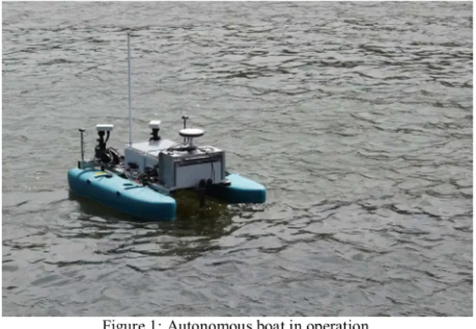
Figure 1: Autonomous boat in operation.

level below the acoustic wavelength used. Although further refinement of the obtained images can be achieved through auto-focus algorithms, these only operate to correct sub-wavelength motion errors, given the accuracy of the navigation system. In order to use all the potential of the available navigation data, a back-projection algorithm that uses the known platform position and attitude during each ping is used.

Knowing the image absolute coordinates eases the task of data integration with other geographic information systems.

II. SYSTEM DESCRIPTION

The autonomous boat is a catamaran like craft (Figure 1) proving high direction stability, smooth operation and several hours of unmanned operation, fulfilling a pre-defined mission plan ([2]). Its size is suitable for, together with the navigation system, executing profiles and other maneuvers with sub-meter accuracy. The boat is modular and easy to assemble in site without the need of any tools. It has two independent thrusters for longitudinal and angular motion providing high maneuverability at low speeds and a maximum speed of 2 m/s. It also embodies an on-board computer for system control, as well as for acquisition and storage of data.

The boat communicates with the shore station (Figure 2) through a high-speed digital radio-link. This link is used to manually control the boat if needed, to initiate the automatic mission, provide the GPS differential corrections and access the surveyed data in real-time.

This floating platform transports an acoustic transducer matrix, placed beneath the waterline, and a set of GPS

Figure 2: Autonomous boat in preparation for a mission and shore station.

receivers together with an inertial sensor to compute its position and attitude with high precision and time resolution.

The SAS system is based on a set of simple acoustic transducers and digital signal processing system for signal generation and acquisition ([3]). The transducers operate at a center frequency of 200 kHz, corresponding to a wavelength of 0.75 cm. As appropriate for synthetic aperture operations, their real aperture is large (approximately 20 degrees), but have a strong front-to-back lobe ratio which is appropriate to minimize the reflections on the near water surface. The effective transducer diameter is 5 cm, which allows for synthetic images with this order of magnitude of resolution in the along-track direction. The usable bandwidth of the transducers (and of the signals employed) is greatly explored thought the use of amplitude and phase compensation to obtain the highest possible range resolution from the system, dus enabling the use of a bandwidth of 20 to 40 kHz with the current transducers.

The transducers are driven by a dedicated FPGA based system. This provides a low cost solution for generating the complex acoustic signals, for controlling the transmitting power amplifiers and the adaptive gain low noise receiving amplifiers, for demodulating and for match filtering the received signals with the transmitted waveform. Each transmit pulse is time-stamped using a real-time clock implemented in the FPGA system that is corrected using the time information and pulse-per-second trigger from a GPS receiver. This enables precise correlation with the navigation data. The results are then supplied to an embedded computer for storage and acoustic image computation. The use of this technology results in a low power consumption system that fits a small box, compatible with the autonomous boat both in size and energy consumption (Figure 3).

III. SONAR MODEL

The sonar transducers are located beneath the boat pontoons, rigidly connected to its structure. The boat is programmed to follow a series of straight lines at a constant velocity, during which acoustic signals are sent and the respective echoes are received by the transducers (Figure 4).

Figure 3: Boat computer, sonar and navigation system.

Each echo contains indistinctive information of an area corresponding to the radiation pattern of the transducers. The transducers are set so a swath of about 50 m is at the boat illuminated broadside. This is known as a strip-map configuration. Track and across-track differentiation is obtained by the use of matched filters. The range matched filter is quite simple and obtained by correlating the received echoes with the transmitted pulse:

( , ) ( , ) ( )

s t_τ =e t_τ ∗p t (1.1)

Here ( )p t is the transmitted pulse, ( , )e t_{τ is the echo signal}

and ( , )s t_{τ is the correlated signal.}

The range resolution will be given by the signal bandwidth and not by its duration. Because of this, it is possible to use longer pulses to reduce the peak transmitted power, maintaining the total signal energy. The pulse maximum length is limited by the nearest distance of interest.

On the other hand, the along-track compression is more complicated. Several along-track echoes are combined regarding their acquisition positions to form a virtual array which in turn is used to synthesize the image ([1]):

1 ˆ( , )_s ( ), f x y s r u u du c   =

∫

Nav Center RX RX RX TX/RX 2 1 T 1 T T2 T3 4 3 4 z y x Pitch Yaw Roll

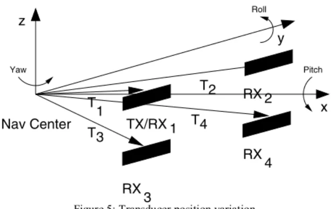
Figure 5: Transducer position variation.

Where ˆf holds the reconstructed image at locations ( , )x y (slant range and along-track coordinates), s is the s

range-compressed image and ( )r u is the distance from the

transmitting transducer to the target and back to the receiver which is given by:

' '

( ) TX( ) RX( )

rτ = T τ −X_σ + X_σ −T τ (1.3)

The image formed in this way has a cross-track resolution of / 2δ =XT c BW and an along-track resolution of

/ 2

AT D

δ = (where c is the speed of sound, BW is the

transmitted signal bandwidth and D is the effective transducer diameter). More importantly the along-track resolution is independent of the target range. To correctly synthesize an image without aliasing artifacts in the along-track dimension, it is necessary to sample the swath with an interval of D/4 (considering the use of only one transducer for transmission and reception). This constrains together with the maximum PRF (given by the more distant echoes) imposes a very slow speed to the boat. For that reason automatic motion control is of high importance for this system.

Sway and surge are kept low trough the boat motion control, but heave is an important component in opposition to tow-fish based sonar systems, because of the waves on the water surface. Yaw variations can also be larger than in tow-fish based systems. Knowing the arm between the boat navigation center (reference for the navigation system), and each transducer (see Figure 5) it is possible to apply the roll, pitch and yaw corrections to the transducers positions by:

'

T = × +R T N (1.4) Where R is rotation matrix associated to the roll, pitch and yaw angles, T is the arm between the transducer and the center of navigation of the boat, N is the absolute position given by the navigation system and _T' _{is the transducer position. The} correct position of each transducer is then used by the image formation algorithm to synthesize the image.

At the moment only a transducer is used for transmission and reception, but we plan to use two transducers arrays to attain a higher survey speed and enable interferometric bottom topography.

Navigation Solution

Trajectory Follow Trajectory Follow

Kalman Filter CP−DGPS INS COMPASS Path reference Velocity reference

Figure 6: Navigation system diagram.

IV. NAVIGATION SYSTEM

The accuracy of the images depends heavily on the ability to correct sensor motion errors. The followed approach is to compensate for these with information from a high accuracy GPS+INS navigation system.

In detail, the navigation system is composed by the following elements: a L1+L2 geodesy grade GPS receiver installed in a static nearby position to operate as a reference station together with another geodesy grade GPS receiver installed in the boat as main position information source. It is capable of receiving the differential corrections from the reference station, perform RTK (real time kinetic) and supply centimeter level accuracy position estimates; an inertial measurement system (INS) with three gyroscopes and three accelerometers; a magnetic compass; two lost cost L1 GPS receivers capable of supplying carrier phase measurements.

All data from these devices are logged for post-processing, besides being used in real-time. The information flow is depicted in Figure 6. Position estimates and heading from the compass is used in the control loop of the boat. This loop has different modes of operation. The most relevant mode actuates the two engines to regulate the speed (measured by GPS) and heading (measured by the compass) in order for the boat to follow straight lines. This loop contains states to estimates the drift due to currents and boat model imperfections ([2]). The carrier phase measurements of the two auxiliary GPS receivers are processed in differential mode to obtain absolute estimates of the boat heading. These are used to calibrate the compass. The inertial measurements are integrated and combined with the L1+L2 GPS positions and calibrated compass measurements in a Kalman filter to produce a full position and attitude navigation solution. The independent heading estimates are needed due to the fact that heading errors are loosely coupled to absolute positions when most of the vehicle motion consists of straight lines. The accuracy of the navigation system is 1 cm in position, 0.02º in roll and pitch and 0.05º in heading.

Using an autonomous boat is therefore advantageous for shallow water bottom mapping, as it allows for using satellite navigation for underwater remote sensing.

V. IMAGE FORMATION

The image formation relies on a back-projection algorithm [8]. This class of synthetic aperture imaging algorithms, although quite computational expensive in comparison with frequency domain algorithms, lends itself very well to non-

3 dB

Echo data Transducer swath

+/−θ

swath for each ping Reconstituted transducer

Superposition with remaining data in correct position given by navigation solution

Figure 7: Back-projection diagram.

linear acquisition trajectories and, therefore, to the inclusion of known motion deviations from the expected path.

The back-projection algorithm enables perfect image reconstruction for any desired path (assuming that rough estimate of the bottom topography is known), since it does not rely on the simple time gating range correction. Instead, it considers that each point in one echo is the summation of the contributions of the targets in the transducer aperture span with the same range.

To reconstruct the image each echo is spread in the image at the correct coordinates (back-projected) using the known transducer position at the time of acquisition (Figure 7). The back-projection algorithm can be formulated as:

( )

(

)

∫

Where w(u) is a weighting factor that compensates the transducer aperture attenuation, yspan is the 3 dB swath size and

r(u) is half the distance between the transmitter to location

(

)

This formulation enables motion compensation for sway, heave and also surge. This last component is of special importance because although the ping-rate is constant the autonomous boat velocity is subject to variations. Yaw, roll and pitch corrections can also be easily introduced. After the transducer position is calculated by 1.4, these parameters only affect the weighting factor. Moreover, the temporal Doppler Effect ([9]) can be included during the echo back-projection, as the instantaneous boat velocity is known. The cross-track pulse compression is independent of the along-track pulse compression in the back-projection algorithm. Therefore, the signal processing chain can be divided in two parts (Figure 8). Furthermore, there are no constraints in using specific transmitted waveforms, such as a chirp. An additional step of deconvolution can be carried out to remove the sinc like response in the range direction that results from the match-filter range compression. This is, however, not suitable for cases were the signal-to-noise rate is low as it emphasizes the high frequency components of the spectrum.

Rough Bottom Height Range Compression

Deconvolution

Back−Projection

Reflectivity Map Raw Echo Data

Navigation Solution

Estimation

Figure 8: Image formation signal flow diagram.

Note that we only have to calculate the points in the image that are affected by each ping. If we consider these points to be the points included in the 3 dB transducer aperture span, a substantial performance gain can be obtained for long survey tracks. If the transducer aperture is large enough compared to the roll and yaw values and the Doppler effect can be ignored, the back-projection of each echo becomes symmetrical to the axis defined by the acquisition position and a small simplification can be made that makes possible to calculate only half of the points affected. Nevertheless, this algorithm is no match for the frequency domain algorithms in terms of processing speed. These have limitation of requiring small errors while following the straight lines and are therefore not suitable for this application.

The main advantages of this algorithm are related to its image quality and ease of incorporation of motion compensation factors. This is true regarding current available personal computers. However, with the back-projection algorithm it is possible to obtain a elegant parallel implementation. Each echo back-projection can be computed separately and then summed together to reconstitute the image. This can lead to a fast implementation using modern FGPA and GPU hardware.

Apart from the described algorithm that can be regarded a coherent back-projection, it is also possible to employ an incoherent back-projection algorithm ([4]):

( )

(

)

∫

Navigation Solution Back−Projection Image Cost Path Cost Estimation Position

(Minimize Total Cost) Range Compressed Echoes

Rough Bottom Height Estimation

Figure 9: Auto-focus block diagram.

This algorithm trades along-track resolution for processing speed and a considerable gain in robustness to unknown platform motion and medium fluctuations. Also, the along-track sampling rate constrain is also lightened and can be higher than D/4without creating aliasing artifacts. The along-track resolution becomes instead ofδ =AT D/ 2:

4.5 XT AT D δ δ λ ⋅ ⋅ = (1.7)

As a by-product, the typical speckle in sonar images is greatly reduced.

VI. AUTO-FOCUS ALGORITHM

The auto-focus algorithm is based on a global contrast optimization technique ([5]) that uses the high grade navigation solution to further refine the trajectory estimative and in turn, improve the obtained image. In fact, the algorithm itself can be regarded as a micro-navigation algorithm since the image quality measurement is exploited to better estimate the boat position. Given the accuracy of the navigation system, the role of the auto-focus system is to correct sub-wavelength motion errors elevating the image quality to the standards needed for high precision applications, such as interferometry.

Starting with the navigation solution provided by the GPS/INS system an optimization algorithm (Nelder-Mead Simplex or Quasi-Newton method) is used to search throughout the solution space to find the position parameters that maximize the image quality (Figure 9). If the boat movement has very low power spectral density at the higher frequencies, one can use the decimated positions or the coefficients of a fitting polynomial as optimization parameters. Otherwise all the coordinates must be used in the search algorithm resulting in cumbersome optimization problem where it is convenient to fix the attention to a zone of interest of the image in question.

The image quality estimate is the quadratic entropy measurement (Quadratic Entropy): This is a measure of image sharpness. The lower the entropy measure, the sharper the image. -40 -30 -20 -10 0 10 20 30 40 -0.2 -0.15 -0.1 -0.05 0 0.05 0.1 0.15 Surge P o si ti o n ( m ) Pulse time (s) -40 -30 -20 -10 0 10 20 30 40 -0.2 -0.1 0 0.1 0.2 Sway P o si ti o n ( m ) Pulse time (s) -40 -30 -20 -10 0 10 20 30 40 -0.02 -0.01 0 0.01 0.02 Heave Pos ition ( m ) Pulse time (s)

Figure 10: Simulated boat 3D position. 2

ˆ _{log ( )}

H _{= −} IP x (1.8)

To calculate the quadratic entropy one needs to estimate the image information potential IP . Instead of making the assumption that the image intensity has a uniform or Gaussian distribution, the probability density function is estimated thought a Parzen window method using only the available data samples: 2 1 1 1 ( ) N N ( _{j i}) j i IP x k x x N = = σ =

∑∑

Wherek x x_σ( − _i)is the Gaussian kernel defined as:

2 2 ( ) 2 1 ( ) 2 i x x i k x x e σ σ πσ − − − = (1.10)

Because this method of estimation requires a computational intensive calculation of the sum of Gaussians, this is implemented through the Improved Fast Gaussian Transform described in [6].

We know beforehand that the solution can not be very far from the initial position estimative. So a similarity measure is used between the estimated path and the measured path. The total objective cost also includes this path cost which acts as a regularization factor of the image cost function and eases the solution convergence. For this similarity measure we used the correntropy function described in [7] as it does not assume any particular characteristics about the path of the boat:

1 1 _ˆ min ( ) N ( _i) i P w k x x N = = −

∑

Performing an image optimization in this way does not rely on strong targets or any other particular image characteristic or statistical assumption. It also has a good degree of robustness to along-track under-sampling.

To illustrate this algorithm an simulated image constituted with 5 point targets was generated. This simulated image was

Along/Cross track compression A lo n g-T ra c k (m ) Cross-Track (m) 20 22 24 26 28 30 32 -5 -4 -3 -2 -1 0 1 2 3 4 Cross compression A lo n g-T ra c k (m ) Cross-Track (m) 20 22 24 26 28 30 32 -5 -4 -3 -2 -1 0 1 2 3 4

Figure 11: Synthetic aperture image reconstitution through back-projection.

created using the described sonar parameters and an imperfect path with surge, heave and sway as shown in Figure 10 which is representative of a typical boat motion during a mission.

The resulting obtained through the back-projection algorithm is shown Figure 11 in and compared to the uncorrected range-compressed image.

As can be seen the image does not show any motion artifacts and is perfectly reconstituted. Now we can compare the coherent version of the back-projection algorithm with the incoherent if we consider the existence of an unknown source of motion error. With the unknown motion source the back-projection starts to produce artifacts and can be seen a considerable along-track resolution loss is the price to pay for unknown motion errors tolerance (Figure 12). Correcting for motion errors and auto-focusing images stands-out as the best solution.

VII. PROJECT STATUS AND RESULTS

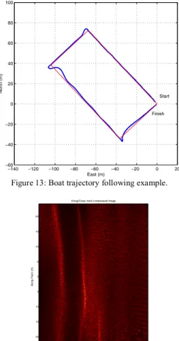
The first test missions were carried in the Douro River. During these missions it was possible to assess the boat tracking performance and sonar imaging capabilities. In Figure 13 is represented the boat trajectory (blue) over the desired trajectory (red). As can be seen there is a slight overshoot at the beginning of the profiles, but otherwise the tracking performance is adequate for together with navigation measurements produce the synthetic sonar image.

Coherent Back-Projection A long-T rac k (m ) Cross-Track (m) 20 22 24 26 28 30 32 -5 -4 -3 -2 -1 0 1 2 3 4

Incoherent B ack-P rojection

A long-T rac k (m ) Cross-Track (m) 20 22 24 26 28 30 32 -5 -4 -3 -2 -1 0 1 2 3 4

Figure 12: Comparison between coherent and incoherent back-projection for images with unknown motion errors.

−140 −120 −100 −80 −60 −40 −20 0 20 −60 −40 −20 0 20 40 60 80 100 East (m) North (m) Start Finish

Figure 13: Boat trajectory following example.

Further refinements on the tracking algorithm will enable better results.

Some images were obtained from the sand banks near the shore (Figure 14 and Figure 15) and from an artificial point target place in the bottom of the river to test the system (Figure 16). All images were further enhanced using the auto-focus algorithm. Due to some limitations it was not possible to use an adequate PRF, which degraded the quality of the images. Nevertheless, is possible to distinguish a strong point like target structure, artificial target, followed by its anchor.

Along/ cross t rack compressed image

A lon g-T rac k ( m ) Cross-Track (m) 16 18 20 22 24 26 28 30 32 -8 -6 -4 -2 0 2 4 6 8

Figure 15: River shore.

A long/Cross track compressed Image

A lon g-T ra c k ( m ) Cross-Track (m) 20 25 30 35 40 45 50 -20 -15 -10 -5 0 5 10 15 20

Figure 14: Sample reflectivity map of a river shore obtained using the described system on one of the first trials.

Along/cross track compressed image A long-T rac k ( m ) Cross-Track (m) 20 25 30 35 40 45 50 -8 -6 -4 -2 0 2 4 6 8

Figure 16: Artificial target and anchor on the bottom of the river.

VIII. CONCLUSION

The obtained results show great potential for this type of platform for synthetic aperture sonar imaging. Not only it is possible to control the boat motion, it is also possible to obtain navigation measurements with precisions in the order of the wavelength used in high resolution sonar systems. The sonar hardware itself and navigation system still need refinement, but the obtained results are promising.

In the future, bottom height mapping will be possible through the use of a double array of transducers and also by exploring the possibility of dual-pass interferometry. In this case the combination of images of the same scene obtained from different positions of the platform will allow the construction of three dimensional maps of the analyzed surfaces.

ACKNOWLEDGMENT

This project has been possible thanks to the contributions of several institutions. The first author is supported by the FCT through the Ph.D. scholarship SFRH/BD/19976/2004/5R38. The authors would like to emphasize the support given by CIIMAR in financing the precision navigation system.

REFERENCES

[1] P. T. Gough, “Unified Framework for Modern Synthetic Aperture Imaging Algorithms”. The International Journal of Imaging Systems and Technology, Vol. 8, pp. 343-358.

[2] N. Cruz, A. Matos, S. Cunha, S. Silva, "ZARCO - Na Autonomous Craft for Underwater Surveys", Proceedings of the 7th Geomatic Week, Barcelona, Spain, Feb 2007.

[3] S. Silva, S. Cunha, A. Matos, N. Cruz, “An In-SAS System For Shallow Water Surveying”, Proceedings of the 7th Geomatic Week, Barcelona, Spain, Feb 2007.

[4] K.Y. Foo, P. R. Atkins, T. Collins, “Robust Underwater Imaging With Fast Broadband Incoherent Synthetic Aperture Sonar”, Proceedings. (ICASSP '03). 2003 IEEE International Conference on Acoustics, Speech, and Signal Processing, Volume 5, 2003 pp. V - 17-20 vol.5 [5] S. A. Fortune, M. P. Hayes, P. T. Gough, “Statistical Autofocus of

Synthetic Aperture Sonar Images using Image Contrast Optimization”, OCEANS, 2001. MTS/IEEE Conference and Exhibition Volume 1, 5-8 Nov. 2001, pp.163 - 169 vol.1.

[6] C. Yang, R. Duraiswami, N. A. Gumerov, L. Davis, “Improved Fast Gauss Transform and Efficient Kernel Density Estimation”, Proceedings of the Ninth IEEE International Conference on Computer Vision (ICCV’03), 2003, pp. 664 - 671 vol.1

[7] W. Liu, P. P. Pokharel, J. C. Principe, “Correntropy: A Localized Similarity Measure”, International Joint Conference on Neural Networks, 2006, pp. 4919 - 4924

[8] A. J. Hunter, M. P. Hayes, P. T. Gough, “A Comparison of Fast Factorised Back-Projection and Wavenumber Algorithms For SAS Image Reconstruction”, Proceedings of the World Congress on Ultrasonics, Paris, France, September 2003.

[9] D. W. Hawkins, P. T. Gough, “Temporal Doppler Effects in SAS”, Sonar Signal Processing, Vol. 26, p. 5, 2004.