www.the-cryosphere.net/7/1741/2013/ doi:10.5194/tc-7-1741-2013
© Author(s) 2013. CC Attribution 3.0 License.
The Cryosphere
Characterization of L-band synthetic aperture radar (SAR)
backscatter from floating and grounded thermokarst lake
ice in Arctic Alaska
M. Engram1, K. W. Anthony1, F. J. Meyer2, and G. Grosse3
1Water and Environmental Research Center, Institute of Northern Engineering, University of Alaska Fairbanks, 306 Tanana
Loop, Fairbanks, AK 99775-7000, USA
2Earth & Planetary Remote Sensing, Geophysical Institute, University of Alaska Fairbanks, 903 Koyukuk Dr., Fairbanks,
AK 99775-7000, USA
3Permafrost Laboratory, Geophysical Institute, University of Alaska Fairbanks, 903 Koyukuk Dr., Fairbanks, AK
99775-7000, USA
Correspondence to:M. Engram ([email protected])
Received: 6 April 2013 – Published in The Cryosphere Discuss.: 22 May 2013
Revised: 13 September 2013 – Accepted: 7 October 2013 – Published: 14 November 2013
Abstract.Radar remote sensing is a well-established method to discriminate lakes retaining liquid-phase water beneath winter ice cover from those that do not. L-band (23.6 cm wavelength) airborne radar showed great promise in the 1970s, but spaceborne synthetic aperture radar (SAR) stud-ies have focused on C-band (5.6 cm) SAR to classify lake ice with no further attention to L-band SAR for this purpose. Here, we examined calibrated L-band single- and quadrature-polarized SAR returns from floating and grounded lake ice in two regions of Alaska: the northern Seward Peninsula (NSP) where methane ebullition is common in lakes and the Arctic Coastal Plain (ACP) where ebullition is relatively rare. We found average backscatter intensities of−13 dB and−16 dB for late winter floating ice on the NSP and ACP, respec-tively, and−19 dB for grounded ice in both regions. Polari-metric analysis revealed that the mechanism of L-band SAR backscatter from floating ice is primarily roughness at the ice–water interface. L-band SAR showed less contrast be-tween floating and grounded lake ice than C-band; however, since L-band is sensitive to ebullition bubbles trapped by lake ice (bubbles increase backscatter), this study helps elucidate potential confounding factors of grounded ice in methane studies using SAR.
1 Introduction and background
Thermokarst (thaw) lakes are abundant in arctic and sub-arctic permafrost lowlands, comprising more than 40 % of the land area in some regions (Grosse et al., 2013). Formed by thermal degradation of permafrost and melting of ground ice, thermokarst lakes range in depth from one to two meters to more than 10 m, largely depending on the ice content of the permafrost in the region and on lake age.
Seasonal ice-cover typically starts forming on lake sur-faces in late October or early November in Arctic Alaska and grows to a maximum thickness of over one meter to two me-ters by late March/early April (Mellor 1982; Jeffries et al., 1994; Arp et al, 2011). Some lakes are shallower than 1–2 m and no liquid water remains at maximum seasonal ice thick-ness, resulting in grounded ice. In lakes that are deeper than the maximum ice thickness, liquid water remains under the thick ice cover all winter (floating ice). Other lakes have a shallow littoral region and freeze to the lake bed close to the shore, while ice floats on liquid-phase water in deeper lake centers.
to year can be used as an indicator of climate change (Hall et al., 1994; Morris et al., 1995; Surdu et al., 2013), serves as a measure of the water balance and the impacts of local disturbances, such as lake drainage, and provides an indica-tor of permafrost health, since an increase in floating lake-ice area alters the heat flux of thermokarst-lake landscape regimes (Jeffries, et al., 2002; Arp et al., 2011, 2012).
A brightness contrast in radar images from floating lake ice versus grounded lake ice was first discovered in the late 1970s with X-band Side Looking Airborne Radar (SLAR) (Sellmann et al., 1975; Elachi et al., 1976; Weeks, 1977) when coastal land areas with lakes were imaged during sea-ice imaging missions. At least two SLAR missions used L-band as well as X-L-band microwave and qualitative exami-nation of radar images found that both wavelengths showed floating ice as bright and grounded ice as dark (Elachi et al., 1976; Sellmann et al., 1977). Elachi et al. (1976) noticed a larger contrast between floating and grounded ice from band than X-band in uncalibrated SLAR, suggesting that L-band radar could be a useful indicator of grounded vs. float-ing ice.
The same phenomenon of high-backscatter return from floating ice and low return from grounded ice was observed in the early 1990s with the advent of calibrated spaceborne SAR, using the C-band VV microwave signal of ERS-1 and ERS-2 (Jeffries et al., 1994; Morris et al., 1995; French et al., 2004). Others have observed this difference using Radarsat-1 C-band HH data (Duguay et al., 2002; Hirose et al., 2008; Arp et al., 2011). Duguay et al. (2002) additionally exam-ined the effect of a varying incidence angle on lake-ice ob-servations and found that a steeper incidence angle (20◦–35◦) provided higher backscatter values from floating ice than a shallow incidence angle (35◦–49◦) for calibrated C-band HH SAR, and that this difference was more pronounced from ice with fewer tubular bubbles. For C-band SAR, backscatter in-tensity after initial ice formation is very low (<−15 dB), and cracks in thin ice can be detected (Hall et al., 1994); however, SAR intensity quickly increases as ice thickens throughout the winter to reach a ceiling of−6 to−7 dB for floating ice. If lake ice grows thick enough to completely ground to the lake bed, the C-band SAR backscatter intensity is low (−14 to−18 dB). Evaluating high or low C-band SAR backscatter from lake ice has become an established method for deter-mining whether a lake retains floating ice all winter or if lake ice is frozen completely to the lake bed in arctic and sub-arctic lakes (Jeffries et al., 1996; French et al., 2004; White et al., 2008; Arp et al., 2012). After a thorough literature search, we could not find any detailed reports that characterized L-band calibrated SAR backscatter intensity from floating and grounded lake ice to follow the early potential that Elachi et al. (1976) reported from L-band airborne radar.
One of the main drivers of radar backscatter intensity is the dielectric constant of the target. Liquid water has a very large real dielectric constant (ε′)compared to ice, so the water–ice interface with its high dielectric contrast has been an obvious
explanation for part of the radar return from floating ice. For L-band,ε≈88 for cold water (Skolunov, 1997) and for C-band,ε′ ≈69, while ice has a dielectric constant of about 3.2 for both C and L-band wavelengths (Leconte et al., 2009). Because of this large difference in the magnitude ofε′for ice and water, there is a strong reflectance of L-band and C-band microwave from the water–ice interface which disap-pears when the lake ice freezes to the ground.
A smooth liquid water surface will reflect microwaves away from the receiving antenna on the satellite due to spec-ular reflection, as demonstrated by calm open water or by newly frozen lakes that appear black in a SAR image. An additional reflector must be present for energy to be turned once again and reflected back to the satellite. Weeks (1978, 1981) and others (Jeffries et al., 1994; Mellor, 1982; Mor-ris et al., 1985, Duguay et al., 2002) have posited that the small (<2 mm diameter) tubular bubbles formed in lake ice by the rejection of dissolved gasses during the freezing pro-cess (Gow and Langson, 1977, Boereboom et al., 2012) play a role in turning radar back to the satellite. Similarly, Engram et al. (2012) showed a positive correlation between L-band backscatter and the abundance of larger (usually 1–100 cm diameter) ebullition bubbles in ice-covered lakes. The same study demonstrated that this positive correlation between single-pol L-band SAR and field measurements of ebullition bubbles in frozen lakes did not exist for C-band VV SAR. Further, they used a polarimetric decomposition to posit that free-phase gas bubbles trapped under ice create a rough sur-face that interacts with Band 3 of the Pauli decomposition (Cloude and Pottier, 1996), resulting in a strong reflectance back to the satellite.
It should be noted that some dark areas on lake ice in un-calibrated C-band SAR images have been documented for floating ice on deep lakes (130 m) in Montana, USA (Hall et al., 1994). Hall et al. attributed these dark areas to thin-ner ice in zones of the lake that had more snow cover and to the different stratigraphy of small tubular bubbles in lake ice than that of northern Alaskan thermokarst lakes. Lakes in more temperate climates have later freeze-up, thinner ice, slower ice growth, possibly more white ice, different patterns of tubular bubbles (Hall et al., 1994) and possibly more thaw-ing and re-freezthaw-ing events durthaw-ing the winter. Dark areas of low backscatter return from these lakes would not indicate grounded ice, but could instead indicate thin, newly-formed ice or ice without small tubular bubbles near the ice–water interface (Hall et al., 1994).
Fig. 1.Study lakes are highlighted in yellow on(a)northern Seward Peninsula (NSP) and(b)Arctic Coastal Plain (ACP) south of Barrow. In panel(a)the large lake in the lower left is Whitefish Maar and the double-lobed lake in the center bottom is Devil Mountain Maar, both of volcanic origin; all other study lakes in both regions are of thermokarst origin. Panel(a)is a Spot 5 mosaic from the Geographic Information Network of Alaska and panel(b)is a scene from 10 July 2008 AVNIR-2 (Advanced Visible and Near Infrared Radiometer type 2).
X-, C- and L-bands with different incidence angles, polar-izations, and acquisition times. It is important to character-ize L-band SAR intensity values from known floating and grounded lake ice, in addition to the established work pub-lished in C-band, in case L-band acquisitions are the only available SAR data. It is furthermore important to study the driving scattering mechanism for scattering in the L-band frequency range in order to better understand the interaction of SAR with lake ice, and in order to identify observation parameters that optimize the contrast between floating and grounded ice. Finally, the magnitude of backscatter intensity decrease that suddenly occurs when lakes freeze to the lake bed is important to know in order to eliminate lakes that ex-hibit a backscatter drop of this magnitude from lake-ice anal-yses targeting methane ebullition (Engram et al., 2012).
Here we examine the value of single-polarized (single-pol) L-band HH backscatter from floating and grounded lake ice. We also use a polarimetric decomposition of quadrature-polarized (quad-pol) SAR data from the Advanced Land Ob-serving Satellite (ALOS) PALSAR L-band SAR to ascer-tain which scattering mechanism (roughness, double-bounce or volumetric scattering) or combination of mechanisms is displayed by floating lake ice. We characterize the differ-ence in L-band backscatter intensity between floating ice and grounded ice for single-pol (HH) and theT11,T22 and T33 polarimetric elements from the coherency matrix of a decomposed quad-pol SAR signal (Lee and Pottier, 2009), and the corresponding dominant scattering mechanism for floating ice for L-band SAR. We discuss morphology at the
ice–water interface as seen in field experiments with lake ice in Fairbanks, Alaska, and consider two physical expla-nations for the dominant L-band SAR scattering mechanism, as seen from a polarimetric decomposition. We compare L-band backscatter intensity values to those of the established C-band VV SAR to determine the utility of L-band SAR in distinguishing between grounded and floating ice, and to possibly gain more understanding of ice–microwave interac-tions at various wavelengths and polarizainterac-tions. Finally, we use statistics to test whether mean backscatter intensity of lake ice is equal two different regions of Alaska.
2 Methods
ice melts. The deep soil organic carbon stocks in the ice-rich Yedoma deposits on the northern Seward Peninsula poten-tially are also higher than soil carbon stocks in the deeper ma-rine, fluvial, and eolian deposits on the Arctic Coastal Plain (Walter Anthony unpublished data). As a result, thermokarst lakes on the northern Seward Peninsula have a higher rate of methane production, resulting in a larger abundance (1.8 seeps-meter−2) of ebullition bubbles trapped in and under
lake ice (Walter Anthony and Anthony, 2013). In contrast, lakes south of Barrow on the Arctic Coastal Plain have sig-nificantly fewer ebullition bubbles (0.4 seeps-meter−2)
in-cluded in their ice cover (Walter Anthony et al., 2012; Wal-ter Anthony and Anthony, 2013). Bubble density was deWal-ter- deter-mined from field data from NSP in fall 2008 and ACP in fall 2009. Including lakes with both high and low numbers of ebullition bubbles was important to this study since ebul-lition may be a confounding factor in isolating floating and grounded ice values in L-band imagery.
Field data on lake-ice thickness, water depth and sedi-ment characteristics were collected for 10 locations on four NSP thermokarst lakes in April 2009 that varied both in bathymetry (deep vs. shallow) and in levels of ebullition bub-bles observed previously by Engram et al. (2012) in field work. We measured ice thickness in auger holes and water depth using sonar (Vexilar LPS-1 Hand-Held Depth Finder) and a weighted measuring tape. Lake sediments were re-trieved with a percussion hammer corer (Farquharson, 2012). In addition to thermokarst lakes, we included in this study the larger Whitefish Maar, a 6 m deep lake on the NSP of vol-canic origin that does not freeze to the bottom in the center (Hopkins et al., 1988). We identified areas of grounded and floating ice on the NSP study lakes using these field measure-ments of grounded and floating ice in April 2009, coincident with SAR imagery, and by using recent ERS-2 image inter-pretation. To identify areas of lakes with grounded vs. float-ing lake ice on the ACP, we used the ERS-2 signal together with field data and remote sensing data from previous pub-lications of C-band VV signal for floating and grounded ice (Mellor, 1983; Jeffries, 1996). Five of the six Arctic Coastal Plain study lakes were featured in early radar research (Sell-mann et al., 1975; Mellor, 1982; Jeffries et al., 1994). We chose one additional lake to increase the sample sizes of lakes with either floating or grounded ice based on recent ERS-2 SAR imagery.
We sampled pixels from L-band Japanese Earth Resources Satellite -1 (JERS-1) scenes from 1993 to 1998 and from both single- and quad-pol L-band PALSAR scenes acquired during 2008–2011 in spring (late March to early April; Table 1). We selected this spring time frame because it represents the period of maximum lake-ice thickness while preceding the onset of melting. ERS-1 and ERS-2 C-band SAR scenes were selected based on acquisition dates closest to L-band SAR acquisitions for verification of grounded lake-ice con-ditions and for comparison of L-band with C-band SAR. The C-band scenes were generally acquired on either the same
day or just a few days apart from L-band acquisitions, except in two cases where a week or more lapsed between acquisi-tions from the different sensors (Table 1).
We used PolSARpro software (v. 4.2.0) to decompose quad-pol L-band images into the 3×3 complex coherency matrix [T3], and compared theT11,T22, andT33 elements
of the coherency matrix (Lee and Pottier, 2009) to SAR single-pol intensity values (Gao, 2010). TheT11,T22 and T33 polarimetric elements are equivalent to the spatially av-eraged versions of Band 3, Band 1, and Band 2 of a Pauli decomposition (Claude and Pottier, 1996), although gener-ally the Pauli bands are expressed as amplitude, which is the square root of the intensity images used in this study. Polari-metric decompositions, such as the Pauli decomposition, pro-vide information about the scattering mechanisms of point and distributed targets by examining the polarization state of transmitted and received energy with the complex scattering matrix [S] (Cloude, 2010; van Zyl and Kim, 2010).
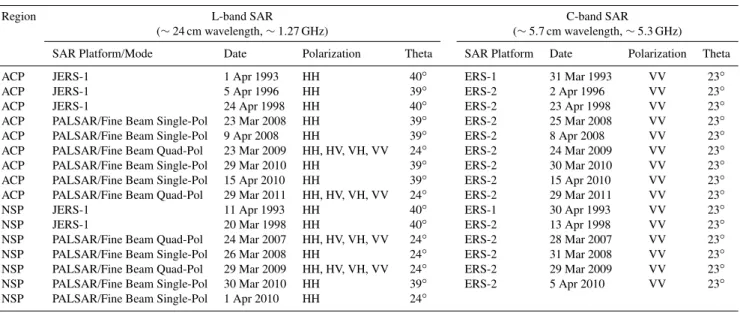
Table 1.SAR data were selected based on data availability over two study areas for late March–April from 1993 through 2011.
Region L-band SAR C-band SAR
(∼24 cm wavelength,∼1.27 GHz) (∼5.7 cm wavelength,∼5.3 GHz)
SAR Platform/Mode Date Polarization Theta SAR Platform Date Polarization Theta
ACP JERS-1 1 Apr 1993 HH 40◦ ERS-1 31 Mar 1993 VV 23◦ ACP JERS-1 5 Apr 1996 HH 39◦ ERS-2 2 Apr 1996 VV 23◦ ACP JERS-1 24 Apr 1998 HH 40◦ ERS-2 23 Apr 1998 VV 23◦ ACP PALSAR/Fine Beam Single-Pol 23 Mar 2008 HH 39◦ ERS-2 25 Mar 2008 VV 23◦ ACP PALSAR/Fine Beam Single-Pol 9 Apr 2008 HH 39◦ ERS-2 8 Apr 2008 VV 23◦ ACP PALSAR/Fine Beam Quad-Pol 23 Mar 2009 HH, HV, VH, VV 24◦ ERS-2 24 Mar 2009 VV 23◦ ACP PALSAR/Fine Beam Single-Pol 29 Mar 2010 HH 39◦ ERS-2 30 Mar 2010 VV 23◦ ACP PALSAR/Fine Beam Single-Pol 15 Apr 2010 HH 39◦ ERS-2 15 Apr 2010 VV 23◦ ACP PALSAR/Fine Beam Quad-Pol 29 Mar 2011 HH, HV, VH, VV 24◦ ERS-2 29 Mar 2011 VV 23◦ NSP JERS-1 11 Apr 1993 HH 40◦ ERS-1 30 Apr 1993 VV 23◦ NSP JERS-1 20 Mar 1998 HH 40◦ ERS-2 13 Apr 1998 VV 23◦ NSP PALSAR/Fine Beam Quad-Pol 24 Mar 2007 HH, HV, VH, VV 24◦ ERS-2 28 Mar 2007 VV 23◦ NSP PALSAR/Fine Beam Single-Pol 26 Mar 2008 HH 24◦ ERS-2 31 Mar 2008 VV 23◦ NSP PALSAR/Fine Beam Quad-Pol 29 Mar 2009 HH, HV, VH, VV 24◦ ERS-2 29 Mar 2009 VV 23◦ NSP PALSAR/Fine Beam Single-Pol 30 Mar 2010 HH 39◦ ERS-2 5 Apr 2010 VV 23◦ NSP PALSAR/Fine Beam Single-Pol 1 Apr 2010 HH 24◦
floating lake ice is indicated by “F” while low backscatter from grounded lake ice is indicated by “G”. Two study lakes
Fig. 2.C-band VV SAR image of thermokarst lakes on the Arctic
Coastal Plain (ACP), Alaska. High backscatter from floating lake ice is indicated by “F” while low backscatter from grounded lake ice is indicated by “G”. Two study lakes are outlined in yellow and pixel sampling locations are rows of uniformly spaced points, shown in contrasting color.
We used the Shapiro–Wilk Test to determine normality on all data distributions. To determine inter-region variability, we compared both grounded and floating-ice backscatter be-tween our two study regions using a statisticalttest for each SAR imaging parameter (wavelength–polarization combi-nations). All statistics were determined by SPSS (v. 19) software. To determine which SAR wavelength–polarization
combination was most useful to distinguish floating and grounded lake ice, we compared the difference between float-ing and grounded lake-ice backscatter values to find the SAR imaging parameters that exhibited the most contrast.
During the timeframe of this study, 1993–2011, we no-ticed that many lakes flipped from springtime grounded-ice to floating-ice status and a few changed from floating-ice to grounded-ice status. Some lakes in the ACP region froze to the bottom in the 1990s but no longer freeze to the bottom in the late 2000s (based on recent C-band SAR data). One of the study lakes, West Twin Lake, was frozen to the lake bed in the 1992 and 1998 spring images, but in 2008 spring images, C-band radar backscatter of about−6 dB signified floating ice. This could be explained by warmer winters, or winters with more insulating snowfall in the more recent past (Walsh et all., 1998; Duguay et al., 2003; Brown and Duguay, 2010; Arp et al., 2012; Surdu et al., 2013). Consequently, pixels from West Twin Lake were classified as grounded ice until 2008, but as floating ice thereafter. Another study lake on the ACP, Kimouksik Lake, was a floating-ice lake in 1993, but low SAR backscatter evinced Kimouksik ice was freezing to the bottom in 2008. This switch from floating ice to grounded ice was a result of a change in water level due to the draining of an adjacent lake between 1992 and 2002. The hydrologi-cal changes of this lake are well documented in Jones (2006). Pixels from Kimouksik Lake were classified as floating ice in 1993, but as grounded ice thereafter.
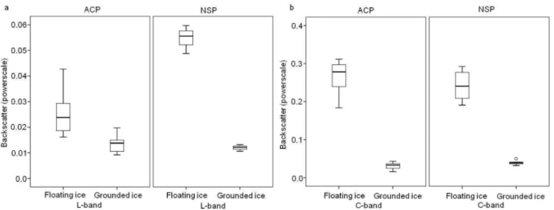
Fig. 3.Boxplots of mean backscatter intensity of all floating and grounded ice from study lakes for each SAR scene from(a)L-band and(b)
C-band. No statistical far-outliers and only one near outlier (panel a NSP, ERS-1, 30 April 1993) indicate that SAR backscatter values from floating and grounded ice in late March–April are similar from year to year. Note different scales onyaxis for(a)and(b).
Although O’Grady Pond is deeper than many thermokarst lakes, we assumed that deep water would not have a differ-ent effect on gas bubbles freezing into surface ice than would a shallow lake. Choosing a lake with no naturally occurring gas ebullition allowed us to control the timing and size of gas bubbles artificially introduced for freezing into the ice column. In March 2013, we shoveled snow off an area of ice on the pond where the ice had been previously removed on 20 January 2013 by Ice Alaska. Following the initial ice har-vest, the ice sheet refroze as clear black ice with a thickness of 27 cm by 16 March 2013. We augured a hole and inserted a plastic tube under the ice attached to a pole 2 m long to allow bubbles to rise in the water column prior to coming to rest under the ice surface as they would in naturally occurring ebullition events. We used air to create bubbles under the ice with a small compressor and a check valve. It should be noted that the flux rate in some of the simulated ebullition events was faster and more short-lived than most flux rates observed in natural ebullition events. We simulated two types of ebul-lition events. In one plot we released a very low volume of gas that formed bubbles approximately one to three centime-ters in diameter. In a second plot we released a larger volume of gas that formed a bubbles on the underside of the ice ap-proximately 10 to 30 centimeters in diameter. We returned to create additional layers of bubbles on 17, 21 and 26th March. We harvested blocks of ice from both areas on 29th March to observe how the rate of ice growth was affected by the insu-lation of gas bubbles, and to reveal the resulting shape of the underside of the lake ice.
3 Results
SAR backscatter values were consistent between years for late March–April scenes for all imaging parameters: box-plots of distributions showed no far-outliers, and only one case of a near outlier (Fig. 3). Backscatter values of sampled pixels for floating and grounded ice averaged from individual
lakes in each SAR scene were normally distributed (Shapiro– Wilk,α=0.05).
We observed that lake sediments in both study regions consisted of organic rich fine-grained sediments (Farquhar-son, 2012; Walter Anthony and Grosse, unpublished data).
From floating lake-ice, L-band single-pol (HH) backscat-ter values showed statistically significant regional variabil-ity and were higher on the NSP (−13 dB) than the ACP (−16 dB). The roughness polarimetric element (T11) of quad-pol L-band SAR was the highest returned signal for floating ice for L-band SAR with a mean backscatter of −9 dB on the NSP and−12 dB on the ACP. In comparison, the values of the polarimetric elements representing double-bounce (T22) and volumetric scattering (T33) were low for floating ice in both regions:−17 dB to−20 dB forT22, and −21 dB to−24 dB forT33 (Table 2 and Fig. 4). Polarimetric elementT11 (roughness) was significantly higher for float-ing ice from lakes in the NSP than from lakes in the ACP (p <0.01), butT22 (double-bounce) andT33 (volumetric) were lower from floating ice in the NSP than ACP (Table 2 and Fig. 4). C-band VV backscatter values for floating ice were statistically identical for both regions (−6 dB) and sub-stantially higher than L-band values for single-pol and all po-larimetric scattering components (Table 2).
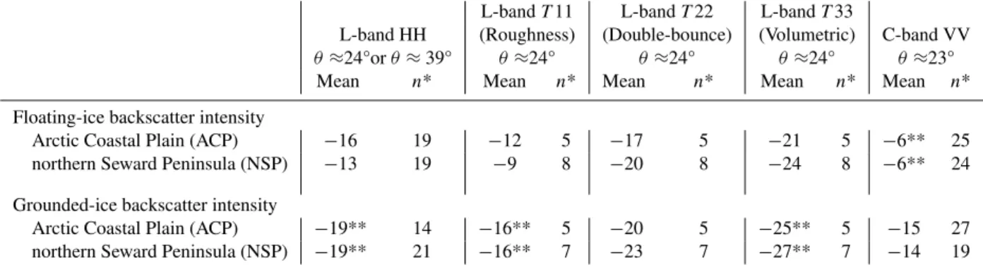
Table 2.Summary of mean SAR backscatter intensity (dB) from floating and grounded lake ice for L- and C-bands from both study regions.
L-bandT11 L-bandT22 L-bandT33
L-band HH (Roughness) (Double-bounce) (Volumetric) C-band VV
θ≈24°orθ≈39° θ≈24° θ≈24° θ≈24° θ≈23°
Mean n* Mean n* Mean n* Mean n* Mean n*
Floating-ice backscatter intensity
Arctic Coastal Plain (ACP) −16 19 −12 5 −17 5 −21 5 −6** 25
northern Seward Peninsula (NSP) −13 19 −9 8 −20 8 −24 8 −6** 24
Grounded-ice backscatter intensity
Arctic Coastal Plain (ACP) −19** 14 −16** 5 −20 5 −25** 5 −15 27
northern Seward Peninsula (NSP) −19** 21 −16** 7 −23 7 −27** 7 −14 19
*Sum of sampled lakes counted from each SAR scene
**Denotes that attest did not reveal a statistically significant difference between the mean backscatter from the ACP and the NSP.
a statistically significant difference between the two regions for grounded ice in L-band HH, L-bandT11(roughness), and T33(volumetric); therefore we assumed equal means (Table 2). Anothert test showed that the average radar brightness of grounded ice on the ACP was not different for the L-bandT11 (roughness) component and C-band. On the NSP, however, means of these two parameters for grounded ice were statistically different (p <0.01). Backscatter intensity from grounded ice on the ACP was significantly different than from the NSP for C-band (p <0.01) and L-bandT22 (double-bounce) (p <0.04).
The contrast (arithmetic difference) between floating and grounded ice SAR backscatter was determined by sub-tracting the grounded-ice sigma-naught backscatter intensity value from that of floating ice, using linear powerscale units. L-band HH mean intensity difference between floating and grounded ice was 0.035 on the NSP and 0.009 on the ACP. These single-pol L-band powerscale values, when converted to decibel log-scale, were the difference between the mean floating and grounded ice intensities of−13 dB and−19 dB on the NSP,−16 dB and−19 dB on the ACP (Table 2). L-band HH contrast between floating and grounded ice in both regions was much lower than C-band contrast. While the log-arithmic scale of decibels prohibits directly subtracting dB values, the C-band contrast was the result of the difference between the floating-ice mean of−6 dB to the grounded ice mean of−14 dB and−15 dB for lakes on the NSP and ACP, respectively.
For all decomposed elements of quad-pol L-band data, backscatter from grounded ice was always lower than from floating ice, but the difference in powerscale units between floating and grounded ice was very small (from−17/−20 dB to−20/−23 dB, ACP/NSP) forT22 (double-bounce) and even smaller (−21/−24 dB to−24/−27 dB ACP/NSP) for T33 (volumetric). The difference between the means of float-ing and grounded ice forT11 (roughness) was largest of the three polarimetric elements, a difference of 0.05 (from−12
to−16 dB) for the ACP, and 0.10 (from−9 to−16 dB) for the NSP (Fig. 5).
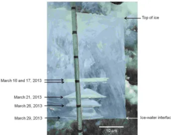
Results from our ebullition simulation field experiment where gas was injected under lake ice at irregular intervals over 14 days, then blocks of ice were harvested to observe ice-bubble stratigraphy and ice morphology, showed that the insulation properties of gas bubbles from ebullition caused upward indentations, or “tenting” on the bottom surface of the ice (Fig. 6). In the plot where we created small diam-eter (1–3 cm) bubbles, this “tenting” or creation of upward-pointing round-tipped, conic shapes in the ice occurred below only a few columns of bubbles. The bottoms of other bubble columns were relatively flat. In the plot with larger diame-ter bubbles (10–30 cm) upward “tenting” where ice growth was slower beneath the insulating gas was observed under every bubble column. These “tents”, or upward bulges in the ice, were identical in scale and shape to others we ob-served in natural ebullition settings in both deep and shallow thermokarst lakes.
4 Discussion
–
Fig. 4.Mean SAR intensity backscatter values in decibels from floating lake ice (open symbols) and grounded lake ice (closed symbols)
from(a)L-band HH from JERS-1 and PALSAR,(b)L-band quad-pol from PALSAR coherency matrix elementsT11 (rectangles),T22 (triangles) andT33 (diamonds) that indicate double-bounce, volumetric scattering, and roughness, respectively,(c)C-band VV from ERS-1 and ERS-2. Incidence angles are(a)39–40 degrees except 24 degrees as noted by concentric circles,(b)23 degrees, and(c)24 degrees. Shaded areas highlight lake ice from the northern Seward Peninsula (NSP) and white areas highlight lake ice from the Alaska Arctic Coastal Plain (ACP). Mean backscatter values are from spring lake ice (late March–April) from study lakes outlined in Fig. 1. Error bars represent standard deviation.
postulated that the roughness involved the ice–water inter-face, our results here show the substantial decrease inT11 backscatter intensity from floating to grounded ice, which provides evidence for the first time that the roughness comes from a rough ice–water interface.
A rough ice–water interface could be caused by uneven ice growth, which can be the result of uneven snow dis-tribution on the ice surface. The highly effective insulating properties of snow make it an important factor in ice growth (Adams and Roulet, 1980; Duguay et al., 2003; Jeffries et al., 2005). Often, wind removes snow from parts of ice-covered lakes and causes snow to drift deeper in other parts. This patchwork of bare ice and snow-covered ice produces ar-eas where ice grows more slowly under insulating snow and more rapidly with less or no snow cover, creating an uneven ice–water interface on the scale of meters.
The cause of a rough ice–water interface could also be ex-plained by ebullition bubbles. Ebullition activity can cause roughness at the ice water interface in two distinct ways. First, as bubbles come to rest under the ice, they cause a rough ice–water interface by creating a pocked water surface, similar to standing waves (Engram et al., 2012). Secondly, as
seen in the results of our ebullition simulation experiment at O’Grady Pond, bubbles that are frozen in the ice cause slower ice growth directly beneath the bubble column, leading to the formation of steep domes of ice that are filled with wa-ter (Fig. 6). These upward-pointing conic and dome shaped “tents” along the bottom surface of the ice were measured up to 4 cm in height in our field experiment, and have been observed 1–30 cm tall in the bottoms of ice blocks harvested over natural ebullition seeps as well. These “tents” are ei-ther filled with water or with gas from subsequent ebullition events, causing roughness.
Fig. 5.Difference in SAR intensity between floating and grounded ice for(a)northern Seward Peninsula (NSP) and(b)Arctic Coastal Plain (ACP). TheT11 component from polarimeteric decomposi-tion of quad-pol L-band data indicates that roughness is the domi-nant scattering mechanism for floating ice for L-band, and is greater in NSP than ACP. C-band clearly shows a larger difference between floating and grounded ice for both regions.
roughness component from floating ice are higher in the NSP then the ACP corroborate the relationship between L-band backscatter and methane flux documented by Engram et al. (2012).
The fact that SAR backscatter was very low (−19 dB) from grounded ice for L-band HH is most likely explained by the low dielectric contrast at the ice–soil interface on the lake bottom. This has been well documented in studies of un-calibrated airborne L-band radar return (Elachi et al., 1976; Weeks, 1978). In the case of grounded lake ice, microwaves pass through snow and lake ice, but with no liquid-phase wa-ter to provide a high dielectric contrast, most of the radar is absorbed by the lake bed instead of reflecting back to the satellite.
For L-band, the signal from grounded ice was a combina-tion of mostly roughness (−16 dB) with some contribution from double-bounce (<−20 dB), while volumetric scatter-ing was negligible (≤ −25 dB), indicating that volumetric scattering from ice itself, in the absence of liquid water below the ice, is close to the noise level of the data (Fig. 4b). This relatively higher L-band T11 roughness backscatter from grounded lake ice could be explained by a reflection from the lake bed. Both regions have fine-grained sediments, as observed by field observations of lake cores in both regions. The small contribution fromT22 (double-bounce) could be explained by L-band reflecting from the lake bed, then re-flecting again from bubbles in the lake ice.
We found the single-pol L-band backscatter from grounded ice (−19 dB) to be lower than that in C-band (−14 to−15 dB). The lower response of L-band vs. C-band from grounded ice is expected, due to the higher penetration power
shaped “tents” due to ice growing at a
Fig. 6.Results of ebullition simulation in a controlled lake-ice
en-vironment. Flat gas pockets sealed in the ice formed from ebullition events on 16 March and 17 March 2013. Subsequently, the topology of the lower ice surface warped into concave, dome-shaped “tents” due to ice growing at a relatively slower rate directly beneath the stack of gas pockets. Ebullition events on 21 and 26 March dis-placed lake water in the tents and filled the tents with gas. No fur-ther ebullition events occurred, yet the bottom surface of the lake-ice sheet was rough, with a 4 cm indentation filled with lake water when this ice block was removed from the lake on 29 March 2013.
of the longer L-band wavelength: penetration distance into a medium is wavelength dependent with the longer wavelength of L-band penetrating deeper than the shorter C-band wave-length. (Ulaby et al., 1986). Another explanation for lower L-band response from grounded ice could be that C-L-band was reflecting from inclusions in the ice, such as tubular bubbles, that may be too small to create a significant scattering con-tribution in L-band.
5 The potential of L-band for detecting grounded and
floating ice
Fig. 7.A frozen thermokarst lake on the Seward Peninsula with floating ice on northern portion of lake and grounded ice at the southern portion shown in L-bandT11 ,T22,T33, and C-band VV images acquired on 29 March 2009. TheT11 roughness component of quad-pol L-band shows some contrast between floating and grounded ice, but it also shows high absolute backscatter, seen as bright areas from high-methane ebullition areas, as determined by field measurements (yellow lines) in October 2008 (Engram et al., 2012). C-band VV shows the strongest contrast between floating and grounded lake ice. Area marked as high ebullition had 11.1 % area of transect with ebullition gas bubbles, low ebullition had 5.1 % of transect area containing bubbles.
ebullition seep density was 1.8 seeps-meter−2while the
den-sity of methane ebullition gas seeps in the ACP was sparser at 0.4 seeps-meter−2.
The difference in magnitude of C-band backscatter be-tween floating and grounded ice was five to thirty-six times higher than the floating-to-grounded ice difference in single-pol L-band (Fig. 5), mostly due to the very high backscatter intensity (−6 dB) from floating ice in C-band. This greater contrast between floating and grounded ice makes C-band VV a more useful tool to distinguish grounded from floating lake ice than L-band SAR. Even the L-band parameter that showed the highest contrast between floating and grounded ice, theT11 roughness component, showed less than half of the contrast than C-band VV showed between floating and grounded ice.
One factor that affects the utility of L-band for distin-guishing grounded vs. floating ice is that it is sensitive to ebullition bubbles trapped by lake ice. In a study of lakes containing different levels of ebullition activity, Engram et al. (2012) observed a positive correlation between backscat-ter and abundance of ebullition bubbles associated with lake ice for L-band single-pol and the roughness component in the Pauli decomposition (analogous to√T11). Similarly, we found higher backscatter in these L-band parameters from high ebullition areas within individual lakes. Figure 7 shows examples of the L-band responses to ebullition and grounded ice in one NSP lake. This higher L-band backscatter response from lake ice with a higher percent area of trapped ebullition bubbles confounds a clear distinction between floating and grounded lake ice. Conversely, grounded lake ice can be a confounding factor for detecting and quantifying ebullition activity in lakes using L-band SAR. The artifact of grounded
ice in ebullition research can be avoided by omitting lakes that show a spring decrease in backscatter.
6 Conclusions
The average backscatter intensity of L-band HH SAR in March is −13 dB for floating ice from the northern Se-ward Peninsula,−16 dB from floating lake ice on the Arctic Coastal Plain, and −19 dB for grounded ice from both re-gions. The dominant L-band scattering mechanism for float-ing lake ice is primarily roughness which occurs at the ice– water interface, as indicated by the strong backscatter from the T11 polarimetric component that decreases when ice freezes completely to the lake bed and liquid water disap-pears.
Acknowledgements. We acknowledge the Alaska Satellite Facility (ASF), both the NASA’s Distributed Data Archive Center and JAXA’s (Japan Aerospace exploration Agency’s) Americas ALOS Data Node for access to SAR data. Access to field sites on the Bering Land Bridge National Preserve was granted by the National Parks Service (permit # BELA-2008-SCI-0002). Thanks to two anonymous reviewers whose comments helped strengthen an earlier version of the manuscript. Funding was provided by NASA Carbon Cycle Sciences NNX08AJ37G and NNX11AH20G and NSF ARC IPY #0732735.
Edited by: D. Hall
References
Adams, W. and Roulet, N.: Illustration of the roles of snow in the evolution of the winter cover of a lake, Arctic, 100–116, 1980. Arp, C. D., Jones, B. M., Urban, F. E., and Grosse, G.:
Hydroge-omorphic processes of thermokarst lakes with grounded-ice and floating-ice regimes on the Arctic coastal plain, Alaska, Hydrol. Process., 25, 17, doi:10.1002/hyp.8019, 2011.
Arp, C. D., Jones, B. M., Lu, Z., and Whitman, M. S.: Shift-ing balance of thermokarst lake ice regimes across the Arc-tic Coastal Plain of northern Alaska, Geophys. Res. Lett., 39, L16503, doi:10.1029/2012gl052518, 2012.
Boereboom, T., Depoorter, M., Coppens, S., and Tison, J.-L.: Gas properties of winter lake ice in Northern Sweden: implication for carbon gas release, Biogeosciences, 9, 827–838, doi:10.5194/bg-9-827-2012, 2012.
Brown, L. C. and Duguay, C. R.: The response and role of ice cover in lake-climate interactions, Prog. Phys. Geogr., 34, 671–704, doi:10.1177/0309133310375653, 2010.
Cloude, S. R. and Pottier, E.: A review of target decomposition theo-rems in radar polarimetry, IEEE T. Geosci. Remote, 34, 498–518, 1996.
Duguay, C. R., Pultz, T. J., Lafleur, P. M., and Drai, D.: RADARSAT backscatter characteristics of ice growing on shallow sub-Arctic lakes, Churchill, Manitoba, Canada, Hydrol. Proc., 16, 1631– 1644, doi:10.1002/hyp.1026, 2002.
Duguay, C. R., Flato, G. M., Jeffries, M. O., Menard, P., Morris, K., and Rouse, W. R.: Ice-cover variability on shallow lakes at high latitudes: model simulations and observations, Hydrol. Proc., 17, 3465–3483, doi:10.1002/hyp.1394, 2003.
Elachi, C., Bryan, M. L., and Weeks, W. F.: Imaging Radar Obser-vations of Frozen Arctic Lakes, Remote Sens. Environ., 5, 169– 175, doi:10.1016/0034-4257(76)90047-x, 1976.
Engram, M., Anthony, K. W., Meyer, F. J., and Grosse, G.: Syn-thetic aperture radar (SAR) backscatter response from methane ebullition bubbles trapped by thermokarst lake ice, Can. J. Re-mote Sens., 38, 667–682, doi:10.5589/m12-054, 2012.
Farquharson, Louise M.: Sedimentology of Thermokarst Lakes Forming Within Yedoma on the Northern Seward Peninsula, Ph.D. diss., University of Alaska Fairbanks, 2012.
French, N., Savage, S., Shuchman, R., Edson, R., Payne, J., and Josberger, E.: Remote sensing of frozen lakes on the North Slope of Alaska, Geoscience and Remote Sensing Symposium, 2004. IGARSS ’04. reProceedings, 2004 IEEE International, 3005, 3008–3011, 2004.
Gao, G.: Statistical Modeling of SAR Images: A Survey, Sensors, 10, 775–795, doi:10.3390/s100100775, 2010.
Gow, A. J. and Langston, D.: Growth history of lake ice in rela-tion to its stratigraphic, crystalline and mechanical structure, U.S. Army, Corps of Engineers, Cold Regions Research and Engineer-ing Laboratory, Hanover, New Hampshire, 24 pp, 1977. Grosse, G., Jones, B., and Arp, C.: 8.21 Thermokarst Lakes,
Drainage, and Drained Basins, in: Treatise on Geomorphology, edited by: Editor-in-Chief: John, F. S., Academic Press, San Diego, 325–353, 2013.
Hall, D. K., Fagre, D. B., Klasner, F., Linebaugh, G., and Liston, G. E.: Analysis of ERS-1synthetic-aperture-radar data of frozen lakes in northern Montana and implications for climate studies, J. Geophys. Res.-Ocean, 99, 22473–22482, 1994.
Hirose, T., Kapfer, M., Bennett, J., Cott, P., Manson, G., and Solomon, S.: Bottomfast ice mapping and the measurement of ice thickness on tundra lakes using C-band synthetic aperture radar remote sensing, J. Am. Water. Resour. As., 44, 285–292, doi:10.1111/j.1752-1688.2007.00161.x, 2008.
Hopkins, D. M.: The Espenberg Maars: a record of explosive vol-canic activity in the Devil Mountain-Cape Espenberg area, Se-ward Peninsula, Alaska, in: The Bering Sea Land Bridge Na-tional Preserve: an archeological survey, edited by: Schaaf, J. M., National Park Service, Alaska Regional Office, 262–321, 1988. Jeffries, M. O., Morris, K., Weeks, W. F., and Wakabayashi,
H.: Structural and stratigraphic features and ERS-1 synthetic-aperture radar backscatter characteristics of ice growing on shal-low lakes in NW Alaska, winter 1991–1992, J. Geophys. Res.-Ocean, 99, 22459–22471, 1994.
Jeffries, M. O., Morris, K., and Liston, G. E.: A method to determine lake depth and water availability on the north slope of Alaska with spaceborne imaging radar and numerical ice growth mod-elling, Arctic, 49, 367–374, 1996.
Jeffries, M. O., Morris, K., and Duguay, C. R.: Lake ice growth and conductive heat flow in central Alaska, Arctic Science Confer-ence Abstracts, 53, 120, 2002.
Jeffries, M. O., Morris, K., and Duguay, C. R.: Lake ice growth and decay in central Alaska, USA: observations and computer simulations compared, Ann. Glaciol., 40, 195–199, 2005. Jones, B. M.: Spatiotemporal Analysis of Thaw Lakes and Basins,
Barrow Peninsula, Arctic Coastal Plain of Northern Alaska., M. A., Department of Geography, University of Cincinnati, Cincin-nati, 105 pp., 2006.
Jorgenson, M. T. and Shur, Y.: Evolution of lakes and basins in northern Alaska and discussion of the thaw lake cycle, J. Geo-phys. Res.-Earth, 112, F02s17, doi:10.1029/2006jf000531, 2007. Jorgenson, T., Yoshikawa, K., Kanevskiy, M., Shur, Y., Ro-manovsky, V. E., Marchenko, S., Grosse, G., Brown, J., and Jones, B. M.: Permafrost Characteristics of Alaska, Permfrost map of Alaska, Ninth International Conference on Permafrost at University of Alaska Fairbanks, 2008.
Leconte, R., Daly, S., Gauthier, Y., Yankielun, N., Bérubé, F., and Bernier, M.: A controlled experiment to retrieve freshwater ice characteristics from an FM-CW radar system, Cold Regions Sci. Technol., 55, 212–220, doi:10.1016/j.coldregions.2008.04.003, 2009.
Mellor, J.: Bathymetry of Alaskan Arctic Lakes: A key to resource inventory with remote sensing methods, Ph.D. diss, Institute of Marine Science, University of Alaska, 1982.
Morris, K., Jeffries, M. O., and Weeks, W. R.: Ice processes and growth history on Arctic and sub-arctic lakes using ERS-1 SAR data, Polar Record, 31, 115–128, 1995.
Sellmann, P. V., Weeks, W. F., and Campbell, W. J.: Use of Side-Looking Airborne Radar to Determine Lake Depth on the Alaskan North Slope, Special Report No. 230. Hanover, New Hampshire: Cold Regions Research and Engineering Laboratory, 1–10, 1975.
Skolunov, A. V.: Frequency-temperature curve of the complex di-electric constant and refractive index of water, Fibre Chemistry, 29, 367–373, 1997.
Surdu, C. M., Duguay, C. R., Brown, L. C., and Fernández Pri-eto, D.: Response of ice cover on shallow lakes of the North Slope of Alaska to contemporary climate conditions (1950– 2011): radar remote sensing and numerical modeling data analy-sis, The Cryosphere Discuss., 7, 3783–3821, doi:10.5194/tcd-7-3783-2013, 2013.
Ulaby, F. T., Moore, R. K., and Fung, A. K.: Radar remote sens-ing and surface scattersens-ing and emission theory, Microwave re-mote sensing : active and passive, edited by: Ulaby, F. T., Artech House, Inc., Norwood, Mass., 608 pp., 1982, 1986.
van Zyl, J. J., and Kim, Y.: Synthetic Aperture Radar Polarimetry, 1st ed., JPL Space Science and Technology Series, edited by: Yuen, J. H., John Wiley & Sons, Inc., Hoboken, New Jersey, 288 pp., 2010.
Walsh, S. E., Vavrus, S. J., Foley, J. A., Fisher, V. A., Wynne, R. H., and Lenters, J. D.: Global patterns of lake ice phenology and climate: Model simulations and observations, J. Geophys. Res.-Atmos., 103, 28825–28837, doi:10.1029/98jd02275, 1998. Walter Anthony, K. M., and Anthony, P.: Constraining
spa-tial variability of methane ebullition in thermokarst lakes us-ing point-process models, J. Geophys. Res.–Biogeosci., 118, doi:10.1002/jgrg.20087, 2013.
Walter Anthony, K. M., Anthony, P., Grosse, G., and Chanton, J.: Geologic methane seeps along boundaries of Arctic per-mafrost thaw and melting glaciers, Nat. Geosci., 5, 419–426, doi:10.1038/ngeo1480, 2012.
Weeks, W. F., Sellmann, P., and Campbell, W. J.: Interesting fea-tures of radar imagery of ice covered north slope lakes, J. Glaciol., 18, 129–136, 1977.
Weeks, W. F., Fountain, A. G., Bryan, M. L., Elachi, C.: Differences in Radar Return From Ice-Covered North Slope Lakes, J. Geo-phys. Res., 83, 4069–4073, 1978.
Weeks, W. F., Gow A. J., and Schertler, R. J.: Ground-truth observa-tions of ice-covered North Slope lakes imaged by radar, Report No. 81-19. Hanover, New Hampshire: Cold Regions Research and Engineering Laboratory, 1–17, 1981.
West, J. J. and Plug, L. J.: Time-dependent morphology of thaw lakes and taliks in deep and shallow ground ice, J. Geophys. Res.-Earth, 113, F01009, doi:10.1029/2006jf000696, 2008.