Estimation of bowhead whale (Balaena mysticetus) population density using spatially explicit capture-recapture (SECR) methods

(1)

UNIVERSIDADE DE LISBOA

FACULDADE DE CIÊNCIAS

DEPARTAMENTO DE ESTATÍSTICA E INVESTIGAÇÃO OPERACIONAL

Estimation of bowhead whale (Balaena mysticetus) population

density using spatially explicit capture-recapture (SECR)

methods

Gisela Vitória Cheoo

Mestrado em Bioestatística

Dissertação orientada por:

Doutor Tiago Marques

(2)

(3)

Acknowledgements

To Len Thomas, my deep appreciation for welcoming me to CREEM (and its cake rituals) and enduring every stupid question I’ve put up. Thank you for being a mentor and taking the necessary time to teach me, although your calendar always looked like a train wreck of a puzzle. I’ll always hear your ’sheesh’ and remember your inability to resist cake time.

No words can describe the joy that is working with Tiago Marques. He was the first person to guide me through the statistical ecology world. For your words of support and guidance, I am sincerely grateful! Among many occasions, thanks for the particular event of dragging a 26 kg bag with broken wheels from St Andrews to Edinburgh’s airport.

To the DEBACA team: Aaron Thode, Alexender Conrad, Cornelia Oedekoven, Danielle Harris, Katherine Kim, and Susanna Blackwell (also Tiago, and Len), for providing the data hereby analysed and giving insight about it. This jolly group of eight has introduced me to new concepts about statistical approaches to estimate densities (and many other concepts I still don’t quite understand!).

To Paul Conn, for discussing a way to implement his superpopulation concept into this thesis. To David Borchers, for the input after the seminar I gave. Thanks also to Richard Glennie for his help building the likelihood formulation.

To every single person that turned my Scottish experience into something I dearly re-member: Amaia Diaz, Carolina Barata, Charles Paxton, Claúdia Faustino, Cornelia Oedekoven, Guilherme Bortolotto, Jessica King, Valentin Popov, Virginia Pujol. Thanks to the St Andrews floorball team. A special thanks to Sean Heath for being a great flatmate, and to Marlene Matthews for being a lovely host during my last week in Scotland.

To Rhona Rodger, and Phil Le Feuvre, always available to help and provide everything needed to properly work at the office.

To all staff involved into making the ISEC 2018 a five star conference, and Len again for letting me attend it.

To Filipe Ribeiro, for also being a mentor – I miss working in the field with "boga-de-boca-arqueada" team.

To all professors and colleagues that somehow helped me through my academic path. A special thanks to Marília Antunes.

(4)

and always made any place feel like home – I am thankful for your friendship.

To Nuno Maia, for your unconditional support and care, and for making my days always brighter! A special thanks to his family too.

To my sister, Mariana Cheoo, for always being there, for your moral support and typically nagging me as older sisters tend to do so. To grandma, Sui Kwong, for being a character of courage and strength (and mostly stubbornness). To mom and dad, Liliana Cheoo, and Calisto Cheoo, for your love and support. Without your invaluable encouragement and sacrifice I could not have done it. Esta tese é para vocês.

Lastly, to the ERASMUS+ programme that allowed me to do part of this thesis in an exceptional research centre, meet new people, and experience life in the country of bagpipes, haggis and cèilidh.

(5)

List of Figures

1.1 Cluster of bowhead whales (Balaena mysticetus). Photo by Julie Mocklin . . . . 3 1.2 Distribution map of Balaena mysticetus. From East to West: Okhotsk Sea,

Spits-bergen Sea, Davis Strait, Hudson Bay, and Bering-Chukchi-Beaufort Sea. Source: http://uk.whales.org/species-guide/bowhead-whale . . . 4 1.3 Example of distance sampling performed in a line transect survey of a certain

whale species: a single observer or a team of observers sail in a specified line transect (centred red line) and record the distances (perpendicular red dashed lines) to detected whales. Black whales indicate detected individuals and therefore recorded distances. Grey whales indicate the presence of animals of interest but observers were unable to detect them. . . 7 1.4 Example of three different types of traps: A) Mist-net representing a multi-catch

trap. B) Cage-trap exemplifying a single-trap. C) Hydrophone (underwater micro-phone) is an example of a proximity detector. Source A: J. Andrew Boyle. Source B: Julian Drewe. Source C: http://ambient.de/en/product/ambient-sound-fish-asf-1-mkii-hydrophone/ . . . 12 1.5 Example of one Directional Autonomous Seafloor Acoustic Recorder (DASAR).

Source: https://www.greeneridge.com/en/ . . . 17 1.6 (a) Alaska State map. Red cross with a circle indicates approximate location

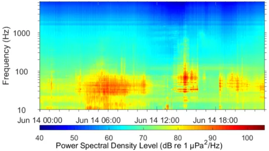
of DASARs deployment. (b) Distribution of DASARs’ deployment locations in 2007-2014 field seasons in northern Alaska coast. There are five main sites with seven-DASAR arrays (red circles), labeled 1 to 5 from west to east. DASARs were labeled A to G from south to north. In 2008, five extra recorders were deployed south of site 1: DASAR locations 1H, 1I, 1J, 1K and 1L (red circles). Inset (5) shows calibration locations at site 5 (black dots) representing DASARs’ locations at single array. Source: Greeneridge Sciences Inc. . . 18 1.7 Example of spectrogram corresponding to vessel traffic and seismic surveys.

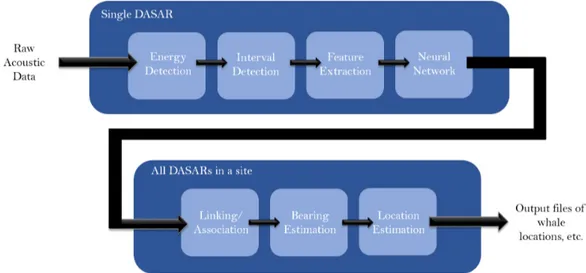
Source: https://www.niwa.co.nz/coasts-and-oceans/research-projects/acoustic-monitoring-whales-dolphins-new-zealand-cook-strait-region . . . 19 1.8 Scheme of automated analysis with seven stages. The first four stages require the

process over a single DASAR, while the last three produces ’call sets’ in order to estimate a call localisation, as well as other features. Source: Thode et al. (2012) 20

(10)

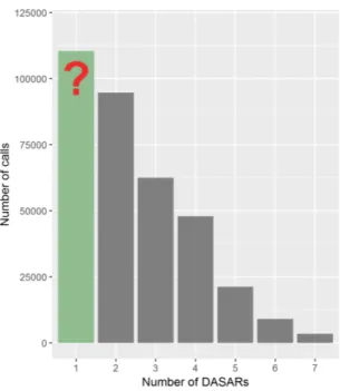
1.9 Percentage distribution of calls detected for the modelling dataset, ranging from 1 to 7 DASARs of site 3, year 2013. (a) Proportion of the number of DASARs an automated call was recorded on. (b) Proportion of the number of DASARs a manual call was recorded on. The proportion of singletons for the automated data is 15.389 times higher than the manual data. . . 22 1.10 Example of the number of calls distribution without the singletons, from 2 to 7

DASARs. The red question mark and green bar indicate a possible higher number of singletons than the one in 2 DASARs according to an exponential decay fitting. 22

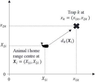
2.1 Schematic representation of a trap location (black cross), home-range centre loc-ation (black whale icon) and distance from trap to centre: dk(Xi) is the distance from the ith animal’s home range centre at Xi to the kth trap at xk. . . 26 2.2 Schematic representation of a spatial trapping grid represented by ’X’ detectors

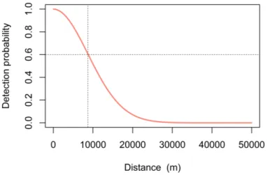
relative to the location of a whale vocalisation pictured by whale icons. . . 29 2.3 Example of a detection function (half-normal distribution). The vertical line

indic-ates σ of the example model (∼8.7 km), meaning the probability of a call produced at that distance from a sensor is about 0.6 (horizontal line) and a near zero chance of detection beyond ∼30 km. . . 29

4.1 Spatial distribution of calls recorded in more than one DASAR for each site. Es-timated call locations are represented by blue dots (in x-y coordinates), DASARs are represented by red letters (A-G or A-M), and the brown line illustrates the Alaskan coast. (a) Sites 2, 3, 4, 5, year 2013 (left to right). (b) Sites 2, 3, 4, 5, year 2014 (left to right). . . 44 4.2 Distribution of the number of calls that were detected at exactly k DASARs (k =

1,..., 11) in each site. (a) Site 1, year 2013. (b) Site 2, year 2013. (c) Site 3, year 2013. (d) Site 4, year 2013. (e) Site 5, year 2013. . . 45 4.3 Percentage distribution of calls recorded at exactly k DASARs (k = 1,...,11). in

each site. (a) Site 1, year 2014. (b) Site 2, year 2014. (c) Site 3, year 2014. (d) Site 4, year 2014. (e) Site 5, year 2014. . . 46 4.4 Linear regression model of an exponential relationship between explanatory

vari-able, number of DASARs (x-axis) and the response varivari-able, number of calls in the logarithmic scale (y-axis). Each black dot corresponds to an observation and the red line matches the regression line, where the grey band area is the 95% confidence level interval for the predicted values. (a) Site 2, year 2013. (b) Site 3, year 2013. (c) Site 4, year 2013. (d) Site 5, year 2013. (e) Site 2, year 2014. (f) Site 3, year 2014. (g) Site 4, year 2014. (h) Site 5, year 2014. . . 47 4.5 Percentage distribution of calls recorded at exactly k DASARs (k = 1,...,7) in site

2. The percentage distribution results from a single sample after subsetting the number of singletons according to a proportion p. (a) Year 2013. (b) Year 2014. . 48

(11)

4.6 Percentage distribution of calls recorded at exactly k DASARs (k = 1,...,7) in site 3. The percentage distribution results from a single sample after subsetting the number of singletons according to a proportion p. (a) Year 2013. (b) Year 2014. . 49

4.7 Percentage distribution of calls recorded at exactly k DASARs (k = 1,...,11) in site 4. The percentage distribution results from a single sample after subsetting the number of singletons according to a proportion p. (a) Year 2013. (b) Year 2014. 49

4.8 Percentage distribution of calls recorded at exactly k DASARs (k = 1,...,7) in site 5. The percentage distribution results from a single sample after subsetting the number of singletons according to a proportion p. (a) Year 2013. (b) Year 2014. . 50

4.9 Call density estimates (number of calls/100 km2) from different approaches: all calls included (circle icons), no singletons included in the dataset (triangle icons); and subset singletons according to a proportion (square icons). Estimates from year 2013 (salmon colour), and estimates from year 2014 (blue colour). . . 51

4.10 Call density estimates (number of calls/100 km2) from simulated data with dif-ferent approaches: all calls included (red), no singletons included in the dataset (green); and subset singletons according to a proportion (blue), and set to ’true’ estimate (purple). Dashed line represents ’true’ density estimate (100 animals/100 km2). . . 53

4.11 Call density estimates (number of calls/100 km2) from the automated data res-ulting from 50 resamples for each year (2013 and 2014) and for each one of the four approaches. The estimates from the simulated data results from 100 simula-tions for each approach (only three are considered: ’no singletons’, ’proportion of singletons’, and ’no transformation’). . . 56

4.12 Population density estimates (number of whales/100 km2 h) with 25% of missing migrating whales and from different approaches: all calls included (circle icon); no singletons included in the automated data (triangle icons); subset singletons according to a proportion in the automated data (square icons); and not perform-ing any subset to the simulated data (cross icons). Estimates from 2013 (salmon colour), and estimates from 2014 (green colour). The mean estimates generated from 100 simulations are blue coloured, and have no year associated. . . 61

4.13 Population density estimates (number of whales/100 km2 h) with 35% of missing migrating whales and from different approaches: all calls included (circle icon); no singletons included in the automated data (triangle icons); subset singletons according to a proportion in the automated data (square icons); and not perform-ing any subset to the simulated data (cross icons). Estimates from 2013 (salmon colour), and estimates from 2014 (green colour). The mean estimates generated from 100 simulations are blue coloured, and have no year associated. . . 62

(12)

4.14 Population density estimates (number of whales/100 km2 _{h) with 45% of missing} migrating whales and from different approaches: all calls included (circle icon); no singletons included in the automated data (triangle icons); subset singletons according to a proportion in the automated data (square icons); and not perform-ing any subset to the simulated data (cross icons). Estimates from 2013 (salmon colour), and estimates from 2014 (green colour). The mean estimates generated from 100 simulations are blue coloured, and have no year associated. . . 63

F.1 Percentage of calls detected from 2 to 11 DASARs on a single resample with no singletons included. (a) Site 2, year 2013. (b) Site 3, year 2013. (c) Site 4, year 2013. (d) Site 5, year 2013. . . 92 F.2 Percentage of calls detected from 2 to 11 DASARs on a single resample with no

singletons included. (a) Site 2, year 2014. (b) Site 3, year 2014. (c) Site 4, year 2014. (d) Site 5, year 2014. . . 93 F.3 Frequency of calls detected per day from one resample. (a) Site 2, year 2013: 3691

detections from a total of 1585 calls detected in 54 days. (b) Site 3, year 2013: 5290 detections from a total of 2543 calls detected in 54 days. (c) Site 4, year 2013: 12337 detections from a total of 4675 calls detected in 55 days. (d) Site 5, year 2013: 5136 detections from a total of 2914 calls detected in 49 days. . . 94 F.4 Frequency of calls detected per day from one resample. (a) Site 2, year 2014: 2259

detections from a total of 970 calls detected in 40 days. (b) Site 3, year 2014: 4206 detections from a total of 1283 calls detected in 47 days. (c) Site 4, year 2014: 7609 detections from a total of 2514 calls detected in 49 days. (d) Site 5, year 2014: 3599 detections from a total of 1230 calls detected in 46 days. . . 95 F.5 Distance from the points of a habitat mask (all points inside the dark blue circle)

to the coastline (brown line) with a buffer of 100 km. (a) Site 2, year 2013. (b) Site 3, year 2013. (c) Site 4, year 2013. (d) Site 5, year 2013. . . 96 F.6 Distance from the points of a habitat mask (all points inside the dark blue circle)

to the coastline (brown line) with a buffer of 100 km. (a) Site 2, year 2014. (b) Site 3, year 2014. (c) Site 4, year 2014. (d) Site 5, year 2014. . . 97

(13)

List of Tables

1.1 Example of a capture history data with n successfully captured individuals in a population with N unknown total animals and 10 sampling occasions. ’1’ rep-resents presence or successful detection in a given sampling occasion; ’0’ means absence or unsuccessful capture. . . 9 1.2 Example of SECR capture histories. Each row corresponds to an object of interest

(for example, animals) and each column a trap. ’0’ indicates no detection at a certain trap, and ’1’ otherwise. Each trap has an associated x-y coordinates. Our data presents this matrix format. . . 11 1.3 Example of SECR capture histories with trapping occasions (1 to S), and traps (1

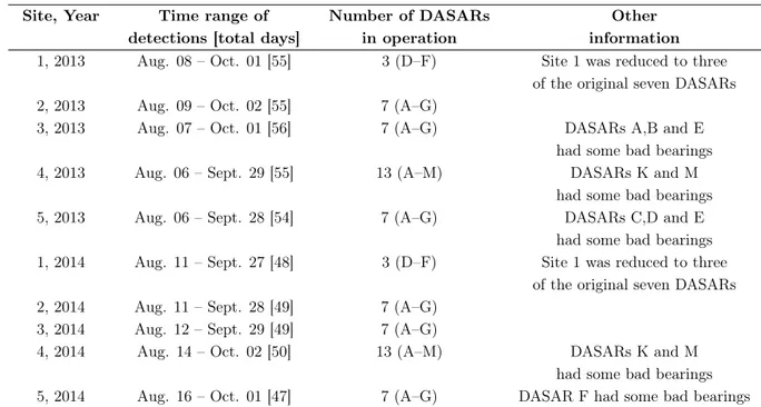
to 10). Each row corresponds to an object of interest (for example, animals) and each column a trap. ’0’ indicates no detection at a certain trap, and ’1’ otherwise. Each trap has an associated x-y coordinates. . . 11 1.4 Additional DASARs information. . . 17

2.1 Example of three candidate detection functions, p_c, for SECR models. The para-meter g0 is common to all functions and represents the intercept, i.e., the probab-ility of detection at a single trap placed in the centre of the home range. d is the distance between an animal home range centre and a trap. σ is the spatial scale parameter and their values are not comparable between functions. . . 28 2.2 Cue rates (calls/h) for sites 2, 3, 4 and 5 of year 2013 and 2014 considering a speed

of 4–5 km/h. . . 32

3.1 Example of a survey with 3 sensors (A, B and C), resulting in seven possible types of capture history. . . 36 3.2 Types of data and approaches that are directly compared for consistency purposes

are marked as ’Check for consistency’. Blank spaces are for general comparisons. 39

4.1 Number of calls recorded in one or multiple DASARs. . . 43 4.2 Proportion of singletons according to predicted values. . . 48

(14)

4.3 Mean density estimates of 2013 with four different approaches: 1) all calls included in the data, 2) excluding singletons; 3) subsetting singletons according to a pro-portion; and 4) truncating singletons. Call density, sigma and intercept estimates are the mean of 50 resamples. . . 52 4.4 Mean density estimates of 2014 with four different approaches: 1) all calls included

in the data, 2) excluding singletons; 3) subsetting singletons according to a pro-portion; and 4) truncating singletons. Call density, sigma and intercept estimates are the mean of 50 resamples. . . 52 4.5 Call density and sigma estimates from simulated capture histories with

corres-ponding coefficient of variation (CV). . . 54 4.6 Call density estimates statistics for each approach and type of data. The

auto-mated data was composed of 400 resamples per approach; the a) and b) simulated data were composed of 400 simulations each per approach. . . 55 4.7 Population density estimates (whales/100km2_{h) from 50 resamples of the}

auto-mated data (2013 and 2014) vs from 100 simulated capture histories. The estim-ates are sorted according to three cue restim-ates and their respective percentages of missing migrating whales (25%, 35% and 45%). . . 58 4.8 Absolute differences of population density estimates (whales/100 km2 h) between

approaches and years for 25% of missing migrating whales. . . 59 4.9 Absolute differences of population density estimates (whales/100 km2 h) between

approaches and years for 35% of missing migrating whales. . . 59 4.10 Absolute differences of population density estimates (whales/100 km2 h) between

approaches and years for 45% of missing migrating whales. . . 59 4.11 Confidence interval (95%) of population densities from simulated data and mean

values of the automated data. . . 60

A.1 Example of output file structure. The first column A corresponds to the column of individual calls; the second group of columns B aggregates 3 columns related to the call and its location; at last, the third group C aggregates sets of 5 columns, each set associated with information of a single DASAR where the call was detected. 76

E.1 SECR parameters description and corresponding interval. . . 85 E.2 Mean and confidence interval of number of calls detected in 1 to 11 DASARs, in

2013 and 2014, from 50 resamples including all calls (singletons and non-singletons). 86 E.3 Mean and confidence interval of number of calls detected in 1 to 11 DASARs, in

2013 and 2014, from 50 resamples with singletons excluded. . . 87 E.4 Mean and confidence interval of number of calls detected in 1 to 11 DASARs, in

(15)

E.5 Summary of exponential equation fitting for all sites and years. . . 89 E.6 Call density and sigma estimates from the automated data vs data from simulated

capture histories. The automated call density estimates are the mean value of 50 resamples. . . 90 E.7 Confidence interval (95%) of population densities from the automated data and

(16)

(17)

Resumo

Na área da ecologia, o estudo de populações naturais é feito através de métodos que têm de ser fundamentalmente precisos e eficazes no que toca à estimação do tamanho e densidade populacional. É importante atualizar e fornecer dados que refletem a realidade do problema em questão. As estimativas resultantes destes métodos são ferramentas que levam à diferença entre uma estratégia de ação que viabiliza a gestão e conservação invertendo o processo de declínio das populações e uma estratégia de conservação falhada. Dada a sua relevância, é importante otimizar os métodos existentes e garantir a eficácia das suas previsões. Se os métodos permitirem a monitorização com a mínima intervenção humana, estaremos a reduzir o esforço, o tempo e os custos necessários, e por essa mesma razão, estes métodos são considerados uma via alternativa preferencial.

A baleia-da-Gronelândia (Balaena mysticetus) pertence à família Balaenidae e é tam-bém conhecida como baleia-da-Gronelândia ou baleia polar. Esta espécie vive em regiões asso-ciadas ao Oceano Ártico e subártico, não ocorrendo no hemisfério Sul. A baleia-da-Gronelândia está classificada na Lista Vermelha de Espécies Ameaçadas (IUCN Red List) como Pouco Preo-cupante (LC – Least Concern). São facilmente identificadas devido ao seu corpo largo, forma arrendonda e por não possuírem barbatana dorsal. Estas baleias apresentam uma tonalidade escura em todo o corpo, exceto os padrões brancos na zona inferior dos maxilares, em partes do corpo da zona ventral e ao redor das suas barbatanas caudais. Os seus padrões brancos aumentam com a idade. Têm uma cabeça triangular quando vista de perfil e um "pescoço" resultante de uma indentação entre a cabeça e a zona dorsal (Rugh & Shelden, 2009). O seu nome comum em inglês, "bowhead whale", surge pela aparência curvada ("bowed") da boca. Além disso, estas baleias são conhecidas pela sua longevidade, tendo sido registado um indivíduo com 211 anos de idade (George et al., 1999). Na região do Alasca, as baleias-da-Gronelândia migram do mar de Bering através do mar de Chukchi para o mar de Beaufort durante o período de migração da primavera/verão, e retornam em meados do final do verão e outono do mar de Beaufort para o mar de Bearing. Apesar das rotas de migração serem bem conhecidas, esta espécie é difícil de ser avistada por passar a maioria do tempo debaixo de água, levando a uma baixa probabilidade de deteção/avistamento. Quando ignorada, esta baixa probabilidade leva à subestimação do tamanho das populações. Contudo, esta espécie é conhecida por emitir vo-calizações que são essenciais para encontrar parceiros durante a época de acasalamento e para ajudar a navegação através do gelo marinho. As vocalizações são de baixa frequência, entre 50 a 500 Hz, mas muito intensas, propensas a serem detetadas a grandes distâncias (Abadi et al., 2014). A produção destes sons distintos faz destas baleias um ótimo exemplo para a aplicação de monitorização acústica passiva.

(18)

O objetivo deste projeto é estimar a densidade populacional das baleias-da-Gronelândia da região de Bearing-Chukchi-Beaufort através da análise de captura-recaptura espacialmente explícita (SECR). Contudo, a densidade calculada pode ser referente a: (i) animais (i.e., indiví-duos); (ii) grupos de animais e (iii) sons. O nosso alvo é estimar inicialmente a densidade (iii) sonora ( ˆDs), sendo posteriormente convertida para uma densidade populacional ( ˆD). A conver-são é feita através da diviconver-são da densidade sonora por dois fatores: (i) taxa de vocalização (ˆr) e (ii) período de tempo considerado da amostra (T):

ˆ D = Dsˆ

ˆ rT.

Os dados analisados nesta tese pertencem a um projeto de nome DEBACA (Density Estimation of Bowhead’s off the Arctic Coast of Alaska), e resultam da colaboração entre a com-panhia americana Greeneridge Sciences Inc e duas instituições académicas – Scripps Institution of Oceanography e a Universidade de St Andrews. O conjunto de dados resulta da colocação de cinco conjuntos de sensors acústicos ao longo da costa do Alasca no mar de Beaufort durante a migração de verão/outono das baleias-da-Gronelândia. Cada um dos conjuntos contém 3 a 13 "DASARs" (Directional Autonomous Seafloor Acoustic Recorders) que gravaram continuamente os sons emitidos pelas baleias. A disposição dos sensores, mais precisamente hidrofones, permitiu a recolha de uma base de dados de acústica passiva durante oito anos (2007–2014) em 5 locais.

Os dados foram divididos segundo a sua análise: os sons foram explorados através de análise manual ou automática. Na análise manual, uma equipa altamente especializada classificou os sons registados, ouvindo as gravações de aúdio e examinando os seus respetivos espetro-gramas ao mesmo tempo. Na análise automática, os dados foram processados através de um algoritmo composto por sete passos, incluindo a classificação e localização dos sons. Contudo, os dados manuais e automáticos apresentam problemas distintos. Nos dados manuais ocorre a não-independência entre os sensores causada por intervenção humana. A não-independência não é consistente com o processo de deteção ao longo dos DASARs, resultando num excesso de sons detetados na totalidade dos DASARs. A independência deverá resultar num padrão decrescente no número de deteções em função do número de DASARs nos quais os sons foram detetados. Os dados automáticos ultrapassam o problema da não-independência, contudo apresentam uma quantidade excessiva de sons "singulares" ("singletons") em relação aos dados manuais (aproxi-madamente mais de 15 vezes). Os sons "singulares" são detetados apenas e somente uma única vez no conjunto de hidrofones. Assume-se que grande parte dos sons "singulares" são, na reali-dade, falsos positivos. Os falsos positivos são sons classificados como sons "biológicos" da espécie de interesse, mas na realidade são provenientes de outra fonte irrelevante para o estudo.

Nesta tese, optámos pela análise de dados automáticos uma vez que excluem o proble-ma da não-independência, além de não ser possível, geralmente, obter dados proble-manualmente em registos de longa duração. Resta-nos então resolver o problema apresentado pela deteção exces-siva de sons "singulares", que por sua vez assume-se que contêm falsos positivos. O problema dos sons "singulares" pode ser abordado das seguintes formas:

1. Analisar todos os dados através de uma análise de captura-recaptura espacialmente explí-cita (SECR), ou seja, ignorando o problema dos "singulares";

(19)

2. Analisar os dados excluindo os sons "singulares";

3. Ajustar um modelo linear com decaimento exponencial aos sons detetados em 2, 3, ..., todos os DASARs de modo a prever o número de sons "singulares". Gerar uma proporção p di-vidindo o número previsto de "singulares" pelo número original de "singulares". Descartar 1 − p de falsos positivos dos sons "singulares";

4. Introduzir uma função de verosimilhança de SECR desenvolvida nesta dissertação que incorpora a truncatura de sons "singulares".

Os pontos 1 a 3 foram analisados através de métodos de SECR com o package secr em R. As estimativas de densidade populacional são validadas através da comparação com dados simulados. O método ad hoc número 3 é considerado o mais fidedigno entre os três, uma vez que resolve parcialmente o problema dos falsos positivos nos sons "singulares". O ponto 1 leva à sobrestimação das densidades, dado que todos os falsos positivos contidos nos "singulares" estão incluídos nos dados analisados. No ponto 2 corremos o risco de subestimar a densidade, uma vez que os sons "singulares" provenientes de baleias são totalmente descartados. No ponto 3 as estimativas correm o risco de serem enviesadas, dado que não é possível saber qual a proporção p de sons "singulares" vindos das baleias-da-Gronelândia. O ponto 4 não foi implementado, no en-tanto estabelecemos as bases para a análise deste conjunto de dados. No caso de implementação da verosimilhança com truncatura de sons "singulares", as estimativas resultantes deste método são apenas referentes a sons detetados em pelo menos dois DASARs. Para trabalho futuro, suge-rimos a inclusão de informação adicional na formulação de SECR, tais como os níveis recebidos dos sons e os ângulos dos sons provenientes da fonte sonora.

Palavras-chave: baleia-da-Gronelândia, estimação de densidade, captura-recaptura espacial-mente explícita, sensores fixos, acústica passiva

(20)

(21)

Abstract

Management and conservation of wildlife populations is a major concern. Population density is a key ecological variable when making adequate decisions about them. A variety of methods can be used for estimating density. Capture-recapture (CR, also known as mark-recapture) methods are a popular choice, but ignoring the spatial component of captures has historically led to problems with resulting inferences on abundance. Spatially explicit capture-recapture (SECR) methods use the spatial information to solve two key problems of classical CR: defining a precise study area where captures occur over and reducing unmodeled heterogeneity in capture probabilities.

Arrays of Directional Autonomous Seafloor Acoustic Recorders (DASARs) recorded calls from the Bearing-Chukchi-Beaufort (BCB) population of bowhead whales during the au-tumn migration. The available passive acoustic dataset was collected over 5 sites (with 3–13 sensors per site) and 8 years (2007–2014), and then processed via both automated and manual procedures. The automated procedure involved computer-processing by a multi-stage detection, classification and localisation algorithm. In the manual procedure, calls were detected and clas-sified by trained staff who manually listened to the recordings and examined spectrograms. The resulting manual data presents some pitfalls for density estimation, including non-independence among sensors caused by human intervention. The non-independence leads to an excess of calls being detected in all DASARs on a site. Data from the automated procedure does not suffer the non-independence issue, but the amount of ’singletons’ is approximately 15 times higher than in the manual data. ’Singletons’ are calls detected exclusively in one sensor and we assume they mostly comprise false positives. False positives are sounds classified as coming from the species of interest, but in reality are something else.

Considering only automated data from 2013 and 2014, several approaches were per-formed to solve the excess of singletons. Density estimation with a standard SECR analysis was conducted according to the following approaches: i) ignoring the singletons problem and analys-ing all calls; ii) removanalys-ing the sanalys-ingletons; and iii) discardanalys-ing a proportion of 1 − p false positives from the singletons. Simulated results were compared to verify the best approach. We also dis-cuss a new approach by developing a SECR likelihood function that accommodates truncation of certain acoustic cues, specifically singletons.

We have laid foundations for the analysis of this dataset, but there are other possible research avenues to explore. Our next steps would include embedding additional information (like received levels and bearing angle) in the SECR formulation.

(22)

Keywords: Bowhead whales, density estimation, spatially explicit capture-recapture, fixed sensor, passive acoustic

(23)

Chapter 1

(24)

1.1 Context of the Problem

The establishment and assessment of management practices concerning wildlife popu-lations must be supported and justified by reliable population estimates. However, population change occurs over time, and it is important to know how it increases or decreases and how many animals of interest are there. One could think population size is enough to support effective ma-nagement and conservation, but much of the theory and methodology concerning population size is to assume populations are well-defined so that one could randomly sample animals in an area and uniquely identify them (Royle, 2011). A popular way to study natural populations is applying in situ monitoring methods. One could resort to traditional abundance estimation methods, such as distance sampling. Bowhead whales are difficult to see as they spend most of their time under the water’s surface. Because a portion of bowhead whales is undetected, this will result in biased abundance estimates. In the concept of population size, animals in a popu-lation typically live and move in territories or home ranges – they are spatially distributed – and the territories or home ranges are, naturally, not accounted in traditional estimation methods. This project seeks to estimate the population density of bowhead whales. This can be achieved with a spatially-explicit capture recapture (SECR) method by juxtaposing in a precisely delin-eated area an array of sensors capable of detecting the presence of the animals. Compared to the traditional abundance estimation methods, this will lead to different implications concerning estimation and interpretation of data. A traditional method, such as capture-recapture, will pro-duce an underestimated population size when there is heterogeneity in capture probability. One of the major sources of heterogeneity is due to the location of the animal’s centre of movement relative to the sensor. The problem of heterogeneity is taken into account in SECR, even though the home range centre is unknown.

The fact that bowheads produce distinctive sounds makes them a suitable candidate for Passive Acoustic Monitoring (PAM) (Cummings & Holliday, 1985). Additionally, the deployment of an array of hydrophones is chosen accordingly to the known migratory routes of bowhead whales (Braham et al., 1980). There is a lot of potential for fixed PAM in studies of cetaceans (whales and dolphins) concerning their ecology, conservation, and movement.

The present case study focuses on PAM to detect the acoustic cues produced by bowhead whales – their sounds – and analyses them with spatially explicit capture-recapture (SECR) methods to estimate population density of bowhead whales in the Arctic Coast of Alaska, spe-cifically in the Bearing-Chukchi-Beaufort (BCB), during the autumn migration.

1.2 Study Species

1.2.1 Characteristics, Taxonomy and Life History

The bowhead whale (Balaena mysticetus) is a cetacean and belongs to the Balaenidae family. Also called Arctic right whale, Greenland right whale or great polar whale, it lives mostly in northern latitudes associated with sea ice, never occurring in the Southern Hemisphere. Bowheads have a classification of least concern (LC), by the IUCN Red List of Threatened

(25)

Species. This species is easy to identify due to their large size, rotund shape and lack of a dorsal fin (figure 1.1). Other unique features such as their triangular head (viewed in profile), and neck (existence of an indentation between the head and back). Their name comes from the bowed appearance of the mouth. Bowheads are black with white patterns on their chins, undersides, around their tail stocks, and on their flukes. Being unique to each individual, these white patterns, mainly around the tail and on the flukes, expand with age (Rugh & Shelden, 2009).

Figure 1.1: Cluster of bowhead whales (Balaena mysticetus). Photo by Julie Mocklin

These cetaceans reach a mean length of 18m and a weight of 45,000 to 73,000 kg (Brownell & Ralls, 1986) and females are larger then males, as in all baleen whale species (Burns et al., 1993). Length of bowhead whales at birth is estimated to be 4-4.5m, length at one year to be 8.2m, length at sexual maturity to be 14m in females, and maximum length to be 20m. The duration of gestation is estimated to be 13-14 months and their sexual activity has been observed in March through May (Nerini et al., 1984). The head of these marine mammals correspond over a third of the bulk of the body with 230 to 360 baleen plates on each side of the mouth, instead of teeth. In order to insulate them, bowheads are protected in blubber 5.5-28 cm thick covered by an epidermis up to 2.5 cm thick (Rugh & Shelden, 2009).

During the mating season, bowheads are vocally active and can hear each other 5-10 km away. Breaching (leaping completely out of the water) and fluke slapping (tail smashes down on the water surface) are usual movements of the mating season that may play a role in attracting a mate or asserting dominance, but the role of these behaviours is not well understood (Rugh & Shelden, 2009).

This species is one of the longest living animals, reaching ages exceeding 100 years, and the oldest individual on record was an astonishing 211 years old (George et al., 1999).

1.2.2 Distribution

There are currently four or five recognized stocks of bowheads which are defined by geographically distinct segments of the species’ total population: the Western Arctic (or Bering-Chukchi-Beaufort stock), Okhotsk Sea in eastern Russia, Davis Strait and Hudson Bay in

(26)

north-eastern Canada (occasionally considered separate stocks) and Spitsbergen in the North Atlantic (figure 1.2) (Heide-Jørgensen et al., 2006; Rugh et al., 2003).

In the Alaskan region, bowhead whales migrate from their Bering Sea wintering grounds through the Chukchi Sea to the Beaufort Sea during spring/summer. The return migration occurs during late spring (April-June) and autumn (September-October) (Moore, 1993). Bowhead whales travel from their eastern Beaufort Sea summering grounds, westward along the coast, and into the Chukchi Sea.

Whales follow open-water leads far from the shore during spring migration. Conversely, the autumn migration is generally near shore and mostly in water depths of 20 to 50 m (Würsig & Clark, 1993).

Figure 1.2: Distribution map of Balaena mysticetus. From East to West: Okhotsk Sea, Spitsbergen Sea, Davis Strait, Hudson Bay, and Bering-Chukchi-Beaufort Sea.

Source: http://uk.whales.org/species-guide/bowhead-whale

1.2.3 Ecology, Behaviour and Physiology

Bowhead whales are planktivorous – planktonic crustaceans, especially copepods and euphausiids, were the most important food items found in bowhead whale diet studies, plus mysids and gammarid amphipods (Lowry et al., 2004). Killers whales (Orcinus orca) are the only predators of bowheads besides humans.

Bowhead whales are skimmers, as they feed on the surface, and sometimes at or near the seafloor. They are capable of engulfing large volumes of water, and swim forward keeping their mouths continuously open when feeding. When closing their mouths, the water is pushed out, trapping prey inside. Their massive tongue sweeps the food off the baleen into a narrow digestive tract (Perrin et al., 2009).

(27)

Being air-breathing mammals, their diving abilities are remarkable – bowheads likely exceed an hour underwater – and they can withstand breaking through ice up to 60 cm thick. During the autumn migration, there is a record for shorter dives (8.65 ± 2.73 min, n=88) com-pared to dive duration during spring (1.7 to > 28 min) (Würsig et al., 1984). Their vocalisations (very-low frequency and very loud calls) are essential to help them find mates or assist in fol-lowing each other when navigating through sea ice. Although extremely vocal, they are solitary animals often travelling alone or in small pods of up to six whales (Rugh & Shelden, 2009).

1.2.4 Interaction with Humans

Bowheads were extremely valuable due to their large size, long baleen and thick blubber. Commercial whalers from the 17th to 19th centuries depleted most stocks of these mammals. In the mid-1970s the International Whaling Commission (IWC) concluded that the harvest by Alaskan Eskimos threatened the existence of the bowhead whale, which was still recovering from a period of open-access exploitation (1848-1914) (Conrad, 1989).

Currently, native Alaskans kill around 40 whales per year through quotas set by the IWC and the Chukotka Natives of Siberia allotted five bowheads per year from the Alaska quota. Independent of this quota, the Canadian government allows a limited hunt of these mammals from the Western Arctic stock and from Davis Strait and Hudson Bay (Rugh & Shelden, 2009).

1.3 Introduction to Density Estimation

Ideally, we would count all the animals of a species of interest from a population in a defined area, resulting in the animal’s density. Suppose we wanted to count all European honey bees in Europe. The exercise of such counting is impossible, as animals move around, and the areas involved are large. So we have to find solutions on sampling approaches and be able to draw inferences about the total population. For instance, imagine a wildlife survey taking place in a study area of size A. A team of investigators randomly deploy a large number of sample plots with total area a, and detect and count n animals. Assuming all animals within the sample plots are counted, then density D is estimated by:

ˆ D = n

a, (1.1)

with the estimated abundance being simply density times the size of the study area

ˆ

N = ˆDA. (1.2)

Frequently, when surveying wild animals, not all animals in the covered areas are detected. If we can estimate the probability p of detecting an animal within a, then density can be estimated as

ˆ D = n

ˆ

(28)

1.3.1 Existing Methods to Estimate Animal Abundance and Density

This section will guide the reader through the existing methods to estimate animal population size, in particular animal abundance and density. The primary goal is to give an outline of the key existing approaches and explain how one obtains abundance/density estimates. Animal abundance was traditionally obtained through visual observations. As a result, most methodologies were focused on visually acquired data. Abundance and density estimates based on visual data were built almost exclusively on one of two inferential methods: capture-recapture/mark-recapture (CR/MR) and distance sampling (DS). The methods applied in this dissertation are a combination of the previous two methods, resulting in spatially explicit capture-recapture (SECR) methods.

The generic term ’detectors’ is used interchangeably throughout this dissertation with the more specific terms ’traps’, ’sensors’, and more specifically ’DASARs’ in further sections. The same happens with the term ’detections’ being described as ’captures’ or ’encounters’. Moreover, ’cue’, ’acoustic cue’, ’sound’ and ’vocalisation’ have the same meaning in this context.

Plot Sampling or Strip Transects

Estimating the size of biological populations can be accomplished with counting. In plot sampling (also known as strip transects), one performs a count of the population of interest over randomly chosen plots. These plots (or strip transects) are usually long, narrow plots or quadrats (Burnham & Anderson, 1984).

Frequently, plot sampling leads to incomplete counts, because these methods are being applied to situations where the key assumption, that all animals in a given area are detected, is false. This results in an underestimation of density. In this method, one searches a plot/strip of area 2Lω (L is the length of the transect and ω is one-half the width of the strip transect) and it is assumed all individuals of interest are detected and counted. These plots may be traversed by an observer on foot, on terrestrial vehicle, on airplane or helicopter, etc. Under the assumption that all individuals are detected and counted, then density D is estimated as

ˆ

D = n

2Lω. (1.4)

However, if some individuals are not detected, i.e., the total number of individuals Nω in the strip of total width 2ω is bigger than the count of detected individuals n (Nω > n), the density estimate is naturally biased low. Note this is just estimator 1.1 where the area size is explicit.

Bias derived from incomplete counts are usually due to:

1. probability of detecting individuals decreasing with distance, x, from the centerline of the strip transect;

2. other factors influencing the detection probability. These variables may include: size, shape, coloration and habits of individuals of interest; level of experience/training of observer;

(29)

variables related to physical setting (e.g., habitat type, time of day, sun angle, among others).

Distance Sampling (DS)

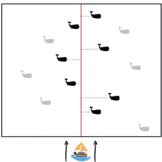
Distance sampling uses the recorded distances to objects of interest obtained by survey-ing lines or points to estimate detectability and hence correct detected counts. If line transects are used, then the perpendicular distances to detected individuals are recorded (figure 1.3); oth-erwise, in the case of point transects, the radial distances from the point to detected individuals are recorded. A point transect may be considered as a line transect of zero length, i.e., a point. The probability of observing an animal decreases as its distance from the observer increases, be-ing the observer a human operator or a sensor. The area effectively searched in distance samplbe-ing is calculated by: A0 = 2µ L, with L being the kms of transect (or other units of distance), and µ as a definition for the effective strip width (distance for which unseen animals located closer to the line than µ equals the number of animals seen at distances greater than µ). Then, density in the area effectively searched is D = n/A0 (Buckland et al., 2012).

Figure 1.3: Example of distance sampling performed in a line transect survey of a certain whale species: a single observer or a team of observers sail in a specified line transect (centred red line) and record the distances (perpendicular red dashed lines) to detected whales. Black whales indicate detected individuals and therefore recorded distances. Grey

whales indicate the presence of animals of interest but observers were unable to detect them.

Distance sampling estimates the area effectively searched, or equivalently the average probability of detection within some fixed truncation distance (Marques et al., 2013). It is important to randomly place a sufficiently large number of line or point transects over the area of interest, so there is a good coverage of the entire area. The recorded distances obtained are then used to model a detection function: g(y), represents the probability of detecting an animal given it is at distance y from the transect. Therefore, the average probability p of detecting an

(30)

animal in the survey area is

p = Z ω

0

g(y)π(y) dy, (1.5)

where ω is the truncated distance from which it is assumed no more detections occur; π(y) is the distribution of distances to all animals (either detected or not) (Buckland et al., 2012). It is assumed that the distribution of animals π(y) is known: uniform for line transects, and triangular for point transects. This is a consequence of a suitable random design. However, in poorly designed surveys, transects may be placed along existing landscape features (e.g., roads, rivers, shorelines, etc). This results in π(y) having an unknown form as animals might present a density gradient due to those features. This will then lead to biased estimates (Marques, 2007). Cue counting is a special kind of distance sampling (Hiby, 1985) – one detects cues produced by animals, instead of counting them directly. Cue counting is a form of distance sampling with a temporal component (Borchers et al., 2010). In this case, it is not possible to determine which individuals produced which cue, therefore the density of cues is estimated alternatively, e.g., whale vocalisations per unit area or per unit of time. This cue estimate is then divided by an independent estimate of the average cue production rate (cue rate – number of sounds per unit of time).

As an example, a survey for songbirds comparing point and line transect sampling was performed in Buckland (2006). Three methods are compared and implemented in both point and line sampling: 1) an observer records birds detected from a point for several minutes; 2) an observer records locations of detected birds ’frozen’ at a single location; and 3) an observer records distances to detected cues (songbursts), rather than birds. The line transect sampling method was more efficient than the point method. Also, the second method was found to be the most efficient of the point sampling methods. Another particular type of distance sampling is suggested in Marques et al. (2013) when animals occur in clusters, hence becoming the object of analysis. The aim here is to obtain a density of animal clusters and then multiply it by an estimate of the mean cluster size in the population. A potential problem arises when large clusters are easier to detect than smaller ones, leading to a potential bias when determining population mean cluster size.

Based on a set of randomly allocated transects over the study area of interest, unbiased density estimates require the following assumptions:

1. animals on the line or at the point are detected with probability 1, i.e., g(0) = 1;

2. animals do not move during the observation process, or the observation process is considered a snapshot, i.e., instantaneous in time;

3. distances are measured without errors;

4. detections are statistically independent events.

Regarding assumption 2), the observation process might happen in a period of time of negligible length, in such a way that animal movement is negligible within the time interval. If

(31)

an observer is faster than the animals themselves, it is safe to assure that existing bias from this source can be ignored. In fact, a simulation study revealed that bias was negligible if mean animal speed was one quarter of that of the observer, but not if animal speed was one half that of the observer (Glennie et al., 2015), although the ratio of animal speed to observer speed for low bias depends on the detection function. In the presence of highly mobile animals, we could face considerable overestimation of density. Moreover, the focus can be directed to unobserved responsive movement, resulting in the overestimation of density if animals are attracted to the observer, and underestimation of density if animals avoid the observers.

In assumption 3), the consequence of measurement errors in estimated distances is similar to the error in animal movement (Marques, 2004). When distances are underestimated and overestimated, the densities will be overestimated and underestimated, respectively. In Marques (2004), it is reported that random errors will typically lead to an overestimation of density.

Finally, assumption 4) is strictly required to estimate the parameters of the detection function model, g(y), by maximum likelihood. Reassuringly, methods are known to be robust to the failure of the independence assumption (e.g. Buckland (2006)).

Capture-recapture (CR) or mark-recapture (MR)

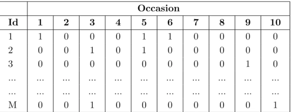
Capture-recapture (also designated mark-recapture) is another approach to estimate abundance. This indirect method involves repeatedly sampling a population of interest over time. CR is performed by marking individuals so they can be recognised in later recaptures. One collects a sample of n individuals, marks and returns them to their habitat. The goal is to obtain their capture history data (also known as individual encounter history data), i.e., a sequence of binary random variables that indicates whether an individual was captured or not during one of these sampling occasions (also named trapping occasions) (table 1.1) (Pradel, 1996).

Table 1.1: Example of a capture history data with n successfully captured individuals in a population with N unknown total animals and 10 sampling occasions. ’1’ represents

presence or successful detection in a given sampling occasion; ’0’ means absence or unsuccessful capture. Occasion Id 1 2 3 4 5 6 7 8 9 10 1 1 0 0 0 1 1 0 0 0 0 2 0 0 1 0 1 0 0 0 0 0 3 0 0 0 0 0 0 0 0 1 0 ... ... ... ... ... ... ... ... ... ... ... ... ... ... ... ... ... ... ... ... ... ... M 0 0 1 0 0 0 0 0 0 1

Depending on what is best suited for each taxon, the recognition from marking can be achieved by photo identification, genetic markers, among others, although many species (e.g.,

(32)

tigers, zebras, some cetaceans) possess individually distinctive natural markings that can be used as markers. The recognition from marking results in an unknown fraction n/N of marked animals, since N is unknown. n is the total number of animals successfully captured (from individual 1 to M). A second sample is drawn. This leads to a proportion p of marked animals for the new sample, which is an estimate of the proportion of marked animals in the population. Hence, we can use the Lincoln-Petersen estimator, one of the oldest and simplest methods based on a single recapture occasion, so an estimate of population size could be given by ˆN = n/p (Krebs et al., 1989). However, one needs to meet multiple unrealistic assumptions to obtain reliable estimates, such as: (i) individuals do not loose marks, (ii) capture does not affect future capture probability, (iii) the population is closed (i.e., no births, deaths, immigration and emigration occur between samples) and (iv) all individuals are equally catchable (equal probability of being detected). This latter assumption has an immense importance, as its failure will produce biased low estimates caused by heterogeneous capture probabilities. The unmodelled heterogeneity in detection probabilities is explained by the tendency of sampled animals being more detectable than others (the opposite of the required iv) assumption), resulting in the overestimation of animal detection probability and underestimation of abundance. The violation of this assumption can lead to lower precision, but also substantial bias (Link, 2003).

Estimates derived from CR cannot readily be converted into density estimates, because there is not a well-defined sampling area. This CR limitation of a non-explicit spatial context leads to an inadequate conversion to density estimation, because animals move freely through space and the area containing the animals exposed to the sampling effort is bigger than the area immediately surrounding the sampling devices. Hence, CR will tend to estimate the size of the population that would at any one time be potentially detectable from the set of traps used, which is most often ill defined.

CR presents other limitations, such as the variation of individual exposure to capture according to the location to their home-range centre and to the location of the sampling devices. The use of CR to estimate population density does not account for: (i) the location of detect-ors/traps; (ii) the location of detections/encounters and (iii) the spatial pattern of individual encounters (or capture history data) (Efford & Fewster, 2013). All this extra information could boost the accuracy and/or precision of the density estimates. This will be discussed in the following sub-section with respect to spatially explicit capture-recapture methods.

Spatially Explicit Capture-Recapture (SECR)

Spatially explicit capture-recapture (SECR) methods represent a natural extension of the CR general framework. The primary goal is to estimate the population density of free-ranging animals and obtain statistical inferences about spatial structure of populations from observed detections of a sample of individuals. These methods are aimed to model animal CR data collected with an array of traps (Efford, 2018).

SECR methods overcome some issues presented by conventional CR, in particular the unmodelled heterogeneity in detected animals and an ill-defined population. In SECR, the spatial location of the location of traps that detected an individual are known, reducing the effect of unmodelled heterogeneity (since part of it is modelled) and making the effective survey area

(33)

estimable.

The primary data for a conventional SECR analysis is (i) the location of traps, and (ii) capture histories, i.e., detections of known individuals on one or more trapping occasions (Efford, 2018). The following table subtly differs from the CR table, since we know the location of the specific traps where the detections occurred (figure 1.2). Depending on the survey design, researchers may need to divide the data into discrete trapping occasions. For example, camera traps sample continuously, so these occasions can be divided in periods of 24 hours (corresponding to the duration of each occasion (1 to S occasions) exhibited in table 1.3).

Table 1.2: Example of SECR capture histories. Each row corresponds to an object of interest (for example, animals) and each column a trap. ’0’ indicates no detection at a certain trap, and ’1’ otherwise. Each trap has an associated x-y coordinates. Our data

presents this matrix format. Traps Id 1 2 3 4 5 6 7 8 9 10 1 1 0 0 0 1 1 0 0 0 0 2 0 0 1 0 1 0 0 0 0 0 3 0 0 0 0 0 0 0 0 1 0 ... ... ... ... ... ... ... ... ... ... ... ... ... ... ... ... ... ... ... ... ... ... M 0 0 0 0 0 0 1 0 0 1

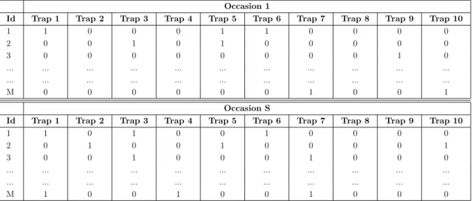
Table 1.3: Example of SECR capture histories with trapping occasions (1 to S), and traps (1 to 10). Each row corresponds to an object of interest (for example, animals) and each

column a trap. ’0’ indicates no detection at a certain trap, and ’1’ otherwise. Each trap has an associated x-y coordinates.

Occasion 1

Id Trap 1 Trap 2 Trap 3 Trap 4 Trap 5 Trap 6 Trap 7 Trap 8 Trap 9 Trap 10

1 1 0 0 0 1 1 0 0 0 0 2 0 0 1 0 1 0 0 0 0 0 3 0 0 0 0 0 0 0 0 1 0 ... ... ... ... ... ... ... ... ... ... ... ... ... ... ... ... ... ... ... ... ... ... M 0 0 0 0 0 0 1 0 0 1 Occasion S

Id Trap 1 Trap 2 Trap 3 Trap 4 Trap 5 Trap 6 Trap 7 Trap 8 Trap 9 Trap 10

1 1 0 1 0 0 1 0 0 0 0 2 0 1 0 0 1 0 0 0 0 1 3 0 0 1 0 0 0 1 0 0 0 ... ... ... ... ... ... ... ... ... ... ... ... ... ... ... ... ... ... ... ... ... ... M 1 0 0 1 0 0 1 0 0 0 Types of Traps

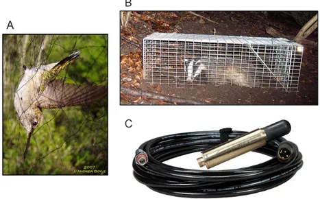
SECR data can be collected with different types of detectors, in addition to physical traps. Efford et al. (2009) describe three categories (figure 1.4):

(34)

duration of a sampling occasion. Therefore, animals are only captured in one trap on any occasion (e.g., mist-nets);

b) Single-trap: these traps hold solely one animal and it stays unavailable to catch other animals once it caught one (e.g., cage-traps);

c) Proximity detectors: technological development opened new possibilities to study species that were historically impossible to study as they were extremely difficult to physically capture. Prox-imity detectors are ’traps’ that record the presence of an animal and leave it free to be detected in other traps on any occasion (e.g., hair snares, camera traps, microphones, and hydrophones).

Figure 1.4: Example of three different types of traps: A) Mist-net representing a multi-catch trap. B) Cage-trap exemplifying a single-trap. C) Hydrophone (underwater

microphone) is an example of a proximity detector. Source A: J. Andrew Boyle. Source B: Julian Drewe.

Source C: http://ambient.de/en/product/ambient-sound-fish-asf-1-mkii-hydrophone/

Proximity detectors are a non-invasive type of sampling since they do not physically capture an animal. As described further in the sub-section 1.5, we performed acoustic sampling with proximity detectors in this dissertation.

1.4 Estimating Cetacean Density from Passive Acoustic Data

There are two major ways to collect data for wildlife abundance estimation: visual observations and trapping. The latter is usually achieved by physically capturing or by photo-ID. The most common survey method is visually based distance sampling and alternatively, mark-recapture by trapping. Both methods are explained in detail in the following section. The problem arises when these methods present limitations in terms of cost, effort and danger to the observers. Taking that into account, PAM offers an alternative survey mode capable of producing high-quality data when other methods fail. Consider the following example: the density estimation of cetaceans. This can be achieved through traditional visual survey methods. Only a portion of the animals present is detected as a result of visual surveys dependence on daylight hours and in relatively good weather. Also the survey observers can only see the animals

(35)

during a very short period when they are at the surface. Visual surveys are performed using a small number of observation platforms with one or a few vessels with a variable survey duration – a few weeks to a few months of the year (Mellinger et al., 2007).

Visual survey results have an additional problem as they may vary dramatically due to clumping of cetaceans into large groups and to their limited spatial and temporal scales. The need for more reliable and effective methods led to the development of alternatives to estimate abundance and/or density. Passive acoustics surpasses those restrictions as many species are also visually cryptic and not amenable to trapping. Nevertheless, many species have detectable and unique sounds that can be used to estimate abundance/density.

In recent years, passive acoustic methods have risen and became increasingly widespread for not only cetacean observation, but also for several other sound producing animals, since: a) sound propagation in water is more efficient than in air, as energy from light is absorbed more than that from sound as it passes through water.

b) visual surveys can be very expensive, usually requiring large investments of ship time and teams of trained observers;

c) many deep-diving cetaceans forage at depths where light does not penetrate well and have to resort to echolocation for foraging, hence becoming detectable for PAM.

Passive acoustic density estimation relies on the sounds (also referred as cues) naturally produced by animals that are detected by sensors and used as a tool to estimate animal abund-ance. In passive acoustic observation, a certain instrument captures cues from the surrounding environment. It is an alternative survey modality that overcomes constraints imposed by visual surveys or physical trapping as the information can be gathered in environments challenging for human observers to work (e.g. deep or polar oceans, presence of fog, recording at night time, among others). Moreover, many species are visually cryptic, others are not amenable to trapping due to lack of effective methods (particularly for recapture in traps) or welfare concerns.

A cue is any identifiable sound, such as calls, whistles, echolocation clicks or feeding buzzes. Acoustic cues are used to identify and/or locate primates (Kalan et al., 2015), birds (Bardeli et al., 2010), bats (Adams et al., 2012), amphibians (Acevedo & Villanueva-Rivera, 2006), fishes (Rountree et al., 2006), and cetaceans (Mellinger et al., 2007). Ultimately, being amenable to automated data collection, passive acoustics is also capable of generating large amounts of data ready to be analysed (Marques et al., 2013).

In passive acoustic monitoring, the object of interest, cue, is used as an indicator of a presence of an animal. In case of ’no detection’, it is not equivalent to an animal being absent, but it suggests that the animal did not necessarily produce a sound, or a sound was produced but not detected. A ’no detection’ may occur if a human operator is not properly listening; if there is a miscalibration of the sensors detecting the cues, if such instruments are used; among others. Usually it is not possible to count the number of individuals directly. Instead, we count the number of vocalisations, although not knowing how many individuals produced them. By using cue rates (estimated number of cues by the duration of the survey) as an indicator, we need to consider these ’multipliers’ in the construction of density estimators. These are factors that convert an indirect estimate into an actual animal density estimate (Marques et al., 2013).

(36)

In passive acoustic surveys, the n in equation 1.3 is the number of detected cues, producing an estimate of density of sounds. The estimator can be divided by an estimate of cue rate to produce an estimate of animal density. Another common multiplier is used to account for ’false positives’ detections, i.e., sounds classified as coming from the species of interest, but in reality are something else. Both multipliers (cue rate and false positives) are incorporated in the density estimator as follows: ˆ D = n(1 − ˆf ) ˆ pcaˆrT , (1.6)

where n is the number of detected sounds during time period T , f is the proportion of detections that are false positives, pc is the probability of detecting a cue in area a, and r is the cue rate that converts density of sounds to animal density.

Obtaining density estimates from passive acoustic data requires: (i) identifying sounds (those being the object of interest) that relate to animal density; (ii) collecting a sample of sounds, n, generated by a well-designed survey protocol; (iii) estimating the rate of false positives, f ; (iv) determining the probability of detection of a cue, p_c; (v) obtaining an estimate of the multiplier r that translates sound density into animal density (Marques et al., 2013).

In this thesis, the population density estimate will be achieved by first acquiring a density estimate of sounds ( ˆDs – number of sounds divided by a study area) and then will be divided by two multipliers: (i) cue rate (ˆr) and (ii) time period over which monitoring took place (T ): ˆ D = ˆ Ds ˆ rT. (1.7)

1.4.1 Applications and Considerations

Defining the object detected

Depending on the acoustic survey, it is possible to consider different objects of interest:

1. animals (i.e., unique individuals);

2. groups of animals or

3. individual sounds.

The target must be chosen according to what is best suited to the species of interest and, naturally, the available resources to collect data. Ultimately we are interested in estimating the density of the first. Note that to transform the second density estimate above (groups) into the first, one needs to obtain a multiplier (mean group size) from acoustically detected groups

(37)

of animals. Similar to the formula 1.7, we would have:

ˆ

D = Dgˆ ˆs

T , (1.8)

with ˆDg being the density estimate of groups of animals, the multiplier ˆs representing a mean group size estimate, and T the considered time period.

Species-specific Factors

Several species-specific factors can influence the performance of acoustic surveys. These factors include:

a) Frequency of the sounds of interest. Bowhead whales frequency ranges from 50 to 500 Hz (Abadi et al., 2014). Sounds below 1 kHz have significantly less seawater absorption loss than sounds above 10 kHz (Francois & Garrison, 1982).

b) Vocal behaviour. Not only vocal behaviour varies with age, gender and season, but also some cetaceans vocalise more frequently or more consistently than others, e.g., male baleen whale species during the breeding season (Mellinger et al., 2007).

c) Sound source level. Larger cetaceans, such as mysticete whales, produce intense vocalisations prone to be detected at longer distances. These can be detected at distances of several tens of kilometers regardless of the arrangement of the hydrophones: on a single hydrophone (Barlow & Taylor, 2005) and much farther – hundreds of kilometers – on hydrophone arrays (Širović et al. (2007), Samaran et al. (2010)). It is important to note that the distance at which a sound is detected is a function of the sound source intensity and also the frequency, because higher frequency sounds suffer much greater transmission loss than low frequency sounds. For example, blue whale calls can be detected hundreds of km away, because they are loud and have low frequency. Sperm whale clicks are also loud, but they are high frequency, so can only be heard at most tens of km away.

d) Sound directionality. Directionality in acoustic signals is best suited for animals using echo-location, such as toothed whales. Bowheads (being a baleen whale) do not use echoecho-location, but a study suggests the existence of directionality of two types of calls (upcalls and downcalls) during the spring migration off Barrow, Alaska (Blackwell et al., 2012). This study indicates calls were slightly stronger ahead of the animals.

1.4.2 Instrumentation Used in Passive Acoustics

There are three types of passive acoustic survey methods:

a) towed acoustic sensors – hydrophones may be attached to a mobile platform (e.g. a ship) to sample a large area. These include a large areal coverage and are simpler to combine acoustic detection with other types of detection, in particular visual;

(38)

less expensive and allow longer periods of observation;

c) gliders and drifting sensors are an intermediate between the previous two sensors. Gliders are free-floating autonomous devices that complete a designed line transect survey (Harris & Gillespie, 2014). They can be equipped with a digital acoustic monitoring instrument to record and process in situ frequency audio to characterize marine mammal occurrence (Baumgartner et al., 2014). These underwater gliders do not require towing (a)) or mooring (b)) and may act as fixed sensors if they move slowly compared with animal speed (Marques et al., 2013). Drifting sensors are buoys equipped with acoustic sensing arrays. The drifting buoys measure ambient noise and detect passive acoustic signals (Pecknold & Heard, 2015).

There are two types of equipment applied in fixed passive acoustic surveys (Mellinger et al., 2007):

a) cabled hydrophones – normally deployed in permanent or semi-permanent installations, providing a constant supply of data in near-real time (Bacon, 1982);

b) autonomous recorders – a hydrophone and a battery-powered data-recording system. These are deployed semi-permanently underwater by mooring, via a buoy or attached to the seafloor. The recorders can operate up to two years and are typically deployed in arrays of 3 to 10 recorders to improve areal coverage and allow the localisation of sound sources. Autonomous recorders must be later retrieved since they store acoustic data internally (Sousa-Lima et al., 2013).

1.5 The Data

1.5.1 Arrays of DASARs

The Shell Exploration and Production Company (SEPCO) commissioned Greeneridge Sciences, Inc. to deploy arrays of fixed ’Directional Autonomous Seafloor Acoustic Recorders’ (DASARs, see figure 1.5) (Greene Jr et al., 2004) to assess the potential Exploration & Production activities, including the impact of airgun sounds on bowhead whales during their westward autumn migration. From 2007 until 2014, Greeneridge Sciences, Inc. deployed, collected, and analysed an extensive acoustic dataset. More than 13 million bowhead calls were detected and localised on up to 40 DASARs. The enormous set of high-quality detected calls analysed in this dissertation was collected by the same autonomous recorders, but only a subset of the recorded vocalisations were considered (years 2013 and 2014).

Arrays of DASARs were deployed at five sites along the Alaskan Beaufort Sea during the late summer/autumn migration route of bowhead whales. The shore distance from the easternmost site to the westernmost was about 280 km – this corresponded from northeast of Kaktovik to northeast of Harrison Bay. Each site was composed of 3 to 13 DASARs (a normal configuration considered 7 DASARs) placed at the vertices of the triangles with 7 km sides and labeled A to G from south to north (up until M if site had 13 DASARs), respectively (figure 1.6). The southernmost DASARs distanced 15-33 km north from the coast and at a water depth of 22-39 m, whereas the northernmost DASAR at each site was 21 km of the southernmost and at a depth of 15-54 m. More information can be found in table 1.4. The installation was executed on