Abstract— Parameter estimation for an assumed sleep
EEG spindle model (AM-FM signal) is performed by using four time-frequency analysis methods. Results from simulated as well as from real data are presented. In simulated data, the Hilbert Transform-based method has the lowest average percentage error but produces considerable signal distortion. The Complex Demodulation and the Matching Pursuit-based methods have error rates below 10%, but the Matching Pursuit-based method produces considerable signal distortion as well. The Wavelet Transform-based method has the poorest performance. In real data, all methods produce reasonable parameter values. However, the Hilbert Transform and the Matching Pursuit-based methods may not be applicable for sleep spindles shorter than about 0.8 sec. Matching Pursuit-based curve fitting is utilized as part of the parameter estimation process.
I. INTRODUCTION
he sleep spindle waveform is one of the hallmarks of human stage 2 sleep EEG and is also one of the few transient EEG events which are unique to sleep. It is commonly known as a group of rhythmic waves within the frequency range of 11-15 Hz, characterized by a progressively increasing, then gradually decreasing, amplitude, which gives the waveform its characteristic name. The time-varying microstructure of sleep spindles may have clinical significance [1] and can be quantified and modeled with a number of techniques. Such quantification/modeling may provide effective biomarkers of neurological disorders, such as Alzheimer’s disease.
Sleep spindles can be regarded as AM-FM signals and can be expressed as:
cos 0
f(t)= A(t) [g(t)]; A(t)≥ (1)
Manuscript received June 30, 2006.This work was supported in part by the EU NoE BIOPATTERN project (project no. 508803).
P. Xanthopoulos,V. Sakkalis,M. Zervakis are with the Department of Electronic and Computer Engineering, Technical University of Crete, Greece. (e-mail:[email protected],[email protected],michal [email protected])
S. Golemati, P. Y. Ktonas, T.Paparrigopoulos, H. Tsekou and C. R. Soldatos are with the Sleep Research Unit, Department of Psychiatry, National Kapodistrian University of Athens, Greece. (e-mail: [email protected], [email protected] , [email protected], [email protected])
M. D. Ortigueira is with UNINOVA, and Department of Electrical Engineering, Univ Nova, Lisboa, Portugal (e-mail: [email protected])
where: A t( )=A0+kacos(2πf ta +θa), as a simple approximation, is a model for the instantaneous envelope (IE), and g t( )=2πf t k0 + bcos(2πf tb +θb), as a simple approximation, is a model for the instantaneous phase [2]. The instantaneous frequency (IF), in rads/sec, is the time derivative of g(t). In that way a spindle waveform can be modeled with six parameters (A0, ka, fa, f0, kb, fb) which can be easily computed from the estimated IE and IF curves.
This paper presents results in the estimation of the above-mentioned six parameters by utilizing four time-frequency analysis methods in simulated and real sleep spindle data.
II. METHODOLOGY
In this part of the paper we discuss the general methodology followed in order to derive the six model parameters from the assumed spindle model.
A. Filtering
Prior to real-data analysis, data filtering is necessary in order to minimize the presence of frequency bands where there is no spindle activity. For this we used a zero-phase bandpass filter (5-22 Hz). The cutoff frequencies were chosen such that the frequency components in the passband 11-15 Hz were passed with unity gain to minimize any spindle waveform distortion.
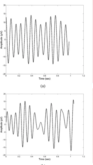
Figure 1 (a) gives an example of a simulated sleep spindle waveform according to the model of Eq. 1, by utilizing parameter values similar to the ones obtained in a preliminary analysis of real data [2]. Figure 1 (b) gives an example of a real sleep spindle waveform (bandpassed data). Observe the similarity of the model to the real data.
B. Analysis
In this work we applied four methods, namely Hilbert Transform (HT), Matching Pursuit with moving window (MP), Complex Demodulation (CD) and Wavelet Transform (WT), to estimate the IE and IF waveforms as described in [3], where results obtained with simulated data were presented. The aim here is to present and discuss results obtained with simulated data exhibiting various levels of noise, as well as results obtained with real data.
Comparative analysis of time-frequency methods estimating the
time-varying microstructure of sleep EEG spindles
P. Xanthopoulos, S. Golemati, V. Sakkalis, P. Y. Ktonas, M. D. Ortigueira, M. Zervakis, T.Paparrigopoulos, H. Tsekou, and C. R. Soldatos
(a)
(b)
Figure 1 Simulated sleep spindle (a) produced with the model of Eq 1, and real sleep spindle (b) after bandpass filtering (5-22Hz).
C. Distortion removal
As briefly discussed in [3], the estimated IE and IF curves contain distortions which must be removed in order to constrain the parameter estimation error. The amount of distortion in each case is method-dependent.
1. Hilbert Transform (HT): Since the Hilbert transform can be viewed as a filter, it will introduce distortion due to its impulse response. In our case, simulation showed that 200 samples (100 from the beginning and 100 from the end of the signal) should be removed to minimize this distortion.
2. Matching Pursuit (MP): In the Matching Pursuit method, distortion is introduced sometimes at the beginning and at the end of the estimated IE and IF waveforms since a smoothing spline is applied in order to interpolate the IE and IF curves. This kind of distortion is case-dependent and we cannot know a priori the signal amount that should be
removed. Empirical analysis showed that removing an amount of 100 samples from the beginning and 100 samples from the end of the signal (a total of 200 samples) is enough in order to minimize this distortion.
3. ComplexDemodulation (CD): In this case, the distortion is due to the lowpass filtering involved in the method. Tests with simulated data showed that 60 samples from the beginning and 60 samples from the end of the signal (a total of 120 samples) should be removed.
4. Wavelet Transform (WT): Since one is dealing with finite-length time series, errors will occur at the beginning and at the end of the wavelet power spectrum, as the Fourier Transform used to efficiently implement the Wavelet Transform assumes the data is cyclic. One solution is to pad the end of the time series with zeroes before performing the Wavelet Transform and then remove them afterward. In this study, the time series is padded with sufficient zeroes to bring the total length N up to the next-higher power of two, thus limiting the edge effects and speeding up the Fourier Transform. Padding with zeroes introduces discontinuities at the endpoints and, as one goes to larger scales, decreases the amplitude near the edges as more zeroes enter the analysis. The cone of influence (COI) is the region of the wavelet spectrum in which edge effects become important and is defined here as the e-folding time for the autocorrelation of the wavelet power spectrum at each scale. This e-folding time is chosen so that the wavelet power for a discontinuity at the edge drops by a factor of e−2 and ensures that the edge effects are negligible beyond this point [4]. For cyclic series, there is no need to pad with zeroes, and there is no COI. As a result of the above, we have to remove about 120 samples (60 from the beginning and 60 from the end of the signal). It should be mentioned that since the distortion introduced by the bandpass filtering of the real data was found to involve about 50 samples at the beginning and at the end of the bandpassed signal (zero-phase filtering), no data removal due to bandpass filtering was implemented because the distorted samples were included in the ones removed for each of the four methods above.
D. Curve fitting
Since the estimated IE and IF waveforms may not be purely sinusoidal, we performed Matching Pursuit-based curve fitting in order to estimate the six parameters that define the spindle model (see Eq. 1).
(
)
cos 2fit fit fit
D = πf t+φ where ffit =0.1:0.005:6 and 0 : : 2
10
fit
π
φ = π
In Figure 3 we show the MP-fitted curves, derived with the four different methods, for a real spindle example.
III. DATA AND RESULTS A. Simulated data
In previous work [3] we tried to estimate the model parameters for some specific examples of simulated, noise-free data. Investigation showed that HT had the lowest average percentage error in estimating the parameters. The average percentage error in MP and CD was below 10%. WT had the highest average percentage error. In this paper, we present results with simulated data that contained noise (10dB and 20dB SNR).
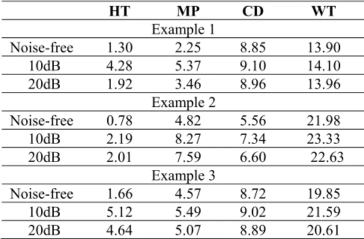
Table 1 shows the average percentage error for the four methods for three specific simulated examples.
TABLE 1 AVERAGE PERCENTAGE ERROR OVER NOISE-FREE AND NOISY
SIMULATED EXAMPLES
HT MP CD WT
Example 1
Noise-free 1.30 2.25 8.85 13.90
10dB 4.28 5.37 9.10 14.10
20dB 1.92 3.46 8.96 13.96
Example 2
Noise-free 0.78 4.82 5.56 21.98
10dB 2.19 8.27 7.34 23.33
20dB 2.01 7.59 6.60 22.63 Example 3
Noise-free 1.66 4.57 8.72 19.85
10dB 5.12 5.49 9.02 21.59
20dB 4.64 5.07 8.89 20.61
As we can see, in all cases, the average percentage error increases as the SNR becomes smaller. The same comparative performance across methods is obtained as in the noise-free data case [3].
B. Real data
Apart from simulated data, the analysis was extended to real data recorded from healthy young adults at the Sleep Research Unit of the Department of Psychiatry at the University of Athens. In Table 2 we can see two such examples. Reasonable parameter values are indicated in bold .
TABLE 2 ESTIMATED PARAMETER VALUES FOR REAL SPINDLES.
REASONABLE PARAMETER VALUES ARE IN BOLD
Parameters HT MP CD WT
Real spindle 1
A0 9.60 9.78 9.49 10.43
fa 2.38 2.39 2.32 2.39
ka 5.28 5.03 5.18 2.10
f0 12.10 12.31 12.35 11.95
fb 2.61 2.49 2.12 2.46
kb 0.78 0.45 0.76 0.51
Real spindle 2
A0 9.07 9.15 9.57 10.31
fa 2.39 2.51 2.18 2.39
ka 5.36 5.01 4.91 4.92
f0 12.73 12.55 12.75 13.57
fb 5.19 4.76 2.35 2.74
kb 0.53 0.19 0.70 0.31
The degree of reasonableness for the parameter values was assessed based on a heuristic visual examination of the estimated curves.
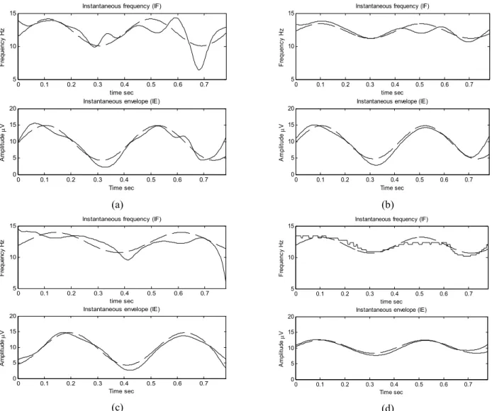
In some cases, where the IE or the IF curve may deviate from a “simple” sinusoidal shape, the curve-fitting method may fail, as expected. In these cases, we may not be able to approximate the sleep spindle waveform with the proposed model, or the curve-fitting method may not reflect obvious sinusoidal characteristics in the data. Figure 2 shows such an example. Here, although the IE curve could be fitted with a plausible sinusoidal model via the proposed methodology, the MP-based curve-fitting method leads to a waveform that fits the global trend in the IF data instead of the “local” sinusoidal changes.
0 0.1 0.2 0.3 0.4 0.5 0.6 0.7 0.8 0.9 5
10 15
Instantaneous frequency (IF)
time sec
F
reque
nc
y
H
z
0 0.1 0.2 0.3 0.4 0.5 0.6 0.7 0.8 0.9 0
5 10 15 20
Instantaneous envelope (IE)
Time sec
A
m
pl
it
ude
μ
V
Figure 2 An example where the MP-based curve-fitting fails to fit sinusoidal characteristics in the IF curve. The solid line is obtained from the analysis process and the dashed one is obtained from the curve-fitting process.
IV. CONCLUSION-FUTURE WORK
The HT method performs best although it requires a removal of 200 samples (about 0.4 sec with a 512 Hz sampling rate), whereas the CD method has higher error percentages but it could be utilized in the analysis of shorter spindles, since it requires a removal of 120 samples (about 0.24 sec with a 512 Hz sampling rate).
some parameters in real spindles. However, it requires the same removal of samples as the HT method. The WT method has the poorest performance with high error rates in simulated data. However, it leads to reasonable values for some parameters in real spindles.
The distortion introduced in each method prevents the analysis of very short spindles (e.g., spindles having length of 0.5 sec). Therefore, given the preliminary results in this paper and in [3], and assuming a sampling rate of 512 Hz, spindles of at least 0.8 sec in length could be analyzed with the CD method, since at least 0.5 sec of data are needed to investigate the presence of at least 2 Hz “oscillations” in the IE and IF curves. Such “oscillations” have been obtained in preliminary work [2].
Although the results reported here look promising, more work should be done in developing appropriate curve-fitting methodology, especially in case the IE and IF curves happen to deviate from “simple” sinusoids. However, in these cases, the proposed sleep spindle model may not hold. Therefore, additional investigation should take place with real data to examine if the proposed model is sufficient to capture important details in the time-varying microstructure of sleep spindles or if appropriate modifications will be needed. Methods like the Empirical Mode Decomposition (EMD) may prove useful in that investigation.
REFERENCES
[1] J C Principe, J R Smith “Sleep spindle characteristics as a function of age,” Sleep 5:73-84 1982.
[2] L Hu, P Ktonas ,“Automated study of sleep spindle morphology utilizing envelope and instantaneous frequency parameters,” Proc., 17th Congress of the European Sleep Research Society, Prague,
Czech Republic, 2004.
[3] P. Xanthopoulos, S. Golemati, V. Sakkalis, P. Y. Ktonas , M. Zervakis and C. R. Soldatos, “Modeling the time-varying microstructure of simulated sleep EEG spindles using time-frequency analysis methods,” Accepted to be presented during the 28th Annual International Conference of the
IEEE Engineering in Medicine and Biology Society, New York, USA, 2006.
0 0.1 0.2 0.3 0.4 0.5 0.6 0.7 5
10 15
Instantaneous frequency (IF)
time sec
F
req
ue
n
c
y
H
z
0 0.1 0.2 0.3 0.4 0.5 0.6 0.7 0
5 10 15 20
Instantaneous envelope (IE)
Time sec
A
m
pl
it
ud
e μ
V
(a)
0 0.1 0.2 0.3 0.4 0.5 0.6 0.7 5
10 15
Instantaneous frequency (IF)
time sec
F
req
ue
n
c
y
Hz
0 0.1 0.2 0.3 0.4 0.5 0.6 0.7 0
5 10 15 20
Instantaneous envelope (IE)
Time sec
A
m
pl
it
ud
e μ
V
(b)
0 0.1 0.2 0.3 0.4 0.5 0.6 0.7 5
10 15
Instantaneous frequency (IF)
time sec
F
reque
nc
y
H
z
0 0.1 0.2 0.3 0.4 0.5 0.6 0.7 0
5 10 15 20
Instantaneous envelope (IE)
Time sec
A
m
pl
it
ude
μ
V
(c)
0 0.1 0.2 0.3 0.4 0.5 0.6 0.7 5
10 15
Instantaneous frequency (IF)
time sec
F
requenc
y
H
z
0 0.1 0.2 0.3 0.4 0.5 0.6 0.7 0
5 10 15 20
Instantaneous envelope (IE)
Time sec
A
m
pl
it
ude
μ
V
(d)