UNIVERSIDADE DE LISBOA
FACULDADE DE CIÊNCIAS
DEPARTAMENTO DE QUÍMICIA E BIOQUÍMICA
Determination of partition coefficients between passive
samplers and the aquatic environment for trace levels of
organic pollutants
Luís Gonçalo Brás Gomes
Mestrado em Química
Especialização em Química Analítica
Dissertação orientada por:
Prof. Dr. Ricardo Silva
Acknowledgements
The realization of this work had important contributions without which it would not be possible to make it a reality and to which I will be eternally grateful.
To Prof. Dr. Ricardo Silva and Dr. Branislav Vrana, for their guidance, support, availability, transmission of knowledge and full collaboration in the accomplishment of this work.
To Dr. Smedes and Dra. Rusina, for the experimental follow-up in the execution of the experiments. To RECETOX research centre and to all those who contributed in some way to my work.
To Jaromír, Alča, Lukáš, Lidka and all the other colleagues, for the fantastic adventures all over the Czech Republic they provided.
To my friends Frederico, Filipe, Maria João, Mariana and Vanessa, for the support and companionship. To Margarida and my parents, brothers and sister, for the emotional strength they provided every day that helped to overcome all the difficulties felt when I was far away from home.
The passive sampling subject present in this dissertation, including experimental work, was developed in the Research Centre for Toxic Compounds in the Environment, located in Brno, Czech Republic.
Abstract
It is of greatest importance to preserve and safeguard the remaining water resources, and to ensure their sustainable management. Hence, environmental monitoring of water is becoming increasingly important and policy programs on water management have been adopted by authorities around the globe with ambitious goals and approaches that can be used for preserving quality of water. Therefore, there is a growing interest in assessing the concentration and distribution of new nonregulated organic contaminants (emerging contaminants) in the environment. The measurement of freely dissolved concentrations using conventional approaches is challenging due to the low concentrations that may be encountered and their temporally variable concentrations. The subsequent laboratory analysis of the sample provides only a snapshot of the levels of pollutants at the time of sampling and episodic pollution events can be missed. Passive sampling technology has been developing very quickly for the past 20 years and, today, these methods represent a viable alternative to traditional sampling methods as they have shown to be promise as tools for measuring concentrations of a wide range of priority pollutants. Depending on sampler design, the mass of pollutant accumulated by a sampler should reflect either the concentration with which the device is at equilibrium or the time-averaged concentration to which the sampler was exposed enabling the estimation of freely dissolved concentrations of contaminants of emerging concern in water.
The use of passive sampling method for estimation of freely dissolved concentrations of emerging contaminants requires the calibration of the passive sampler device. The partition coefficients of a target compound between the passive sampler and water is one of the needs for a successful calibration of the passive sampler device. Measurement of partition coefficients between silicone rubbers and water, Kpw, becomes more difficult as the hydrophobicity of the compound increases. Experimental challenges include long extraction times, sorption to various surfaces and materials, and incomplete dissolution of the compound in the aqueous phase. In order to avoid these artifacts and to shorten experimental time, a series of equilibration experiments of target compounds between the sampler and water in a closed system were performed.
For polycyclic aromatic hydrocarbons (PAHs) and personal care products (PCPs), polymer-water partition coefficients were determined in ultra-pure water for AlteSil™ silicone rubbers using equilibration by both compound release and uptake kinetics. The direct contact method is used to equilibrate polymers under enhanced pressure. A spiked silicone rubber sheet is sandwiched between two other unspiked sheets to decrease its concentration and perform new equilibration process for polymer-water partition coefficients estimation. Estimated polymer-water partition coefficient values are in good agreement with the values from different experimental methods and with the literature values. Also, a study of temporal evolution of the concentration of target compounds in the aqueous phase and the wall of the bottles was performed. However, only sampling rates from equilibration experiments were estimated.
The Monte Carlo method is used to evaluate the uncertainty of the complex determination of partition coefficients. For Monte Carlo simulation, a mathematical model is built to describe all interactions between input quantities that affect partition coefficients determination. From that model, mathematical samples from each parameter are generated, which represent estimated values of the input variables, and combined to estimate the distribution of the measurement result. Probability density functions are used to represent the statistical distribution of each input parameter. The results from the 105 Monte Carlo trials are used to estimate the output quantity value and its associated uncertainty.
Resumo
Nos dias de hoje, contamos com o acesso a água limpa e segura para consumo e utilidade em todos os aspectos das atividades da nossa rotina diária. No entanto, a água é também um meio de transporte e receptor dos produtos resultantes da actividade humana, os quais são disseminados pelo meio ambiente. É, portanto, da maior importância preservar e salvaguardar os recursos hídricos que restam e assegurar a sua gestão de uma forma sustentável. Como tal, a monitorização ambiental da água está a tornar-se cada vez mais importante, e políticas de gestão da água têm vindo a ser adoptados pelas autoridades responsáveis em todo o mundo com metas e abordagens cada vez mais ambiciosas. Com o surgimento de novos contaminantes ambientais, tem havido um interesse cada vez maior em avaliar a concentração e distribuição de compostos que não constam nas listas de compostos prioritários, isto é, não regulados no meio ambiente.
A medição de concentrações de contaminantes biodisponíveis na água usando métodos de amostragem convencionais é desafiante porque estas concentrações são, muitas vezes, baixas ao ponto de não serem detectáveis através do uso das técnicas instrumentais analíticas existentes, a não ser que sejam amostrados e concentrados volumes muito grandes de água. A monitorização destes compostos também é dificultada pela variação temporal da concentração dos compostos na água devido a variáveis externas, fazendo com que a análise laboratorial forneça apenas informação pontual dos níveis de poluentes no momento da amostragem o que torna indetetáveis as contaminações episódicas. A amostragem passiva da água supera estes problemas devido ao facto de apesar de o dispositivo de amostragem ter um volume pequeno, tem uma capacidade de absorção do analito muito elevada e é capaz de medir concentrações médias ponderadas ao longo do tempo de amostragem que se pode estender por várias semanas. A amostragem passiva é uma tecnologia baseada no fluxo livre de moléculas de analito a partir da matriz aquosa para o amostrador passivo. Os dispositivos utilizados para amostragem passiva baseiam-se na difusão dos compostos através de uma barreira de difusão ou na permeação através de uma membrana. As forças motrizes de difusão e os mecanismos de separação são resultado dos diferentes gradientes de concentração, pressão, temperatura e força electromotriz, os quais podem ser reduzidos a gradientes de potencial químico fundamentais do analito entre os dois meios, resultando no enriquecimento e isolamento de analitos no meio receptor: o amostrador passivo.
A tecnologia de amostragem passiva tem vindo a desenvolver-se muito rapidamente nos últimos 20 anos e já constitui uma alternativa viável aos métodos de amostragem tradicionais, uma vez que se desenvolveram ferramentas de medição de concentrações aquosas de uma ampla gama de poluentes. Dependendo do tipo de dispositivo de amostragem passiva, a massa de poluente acumulada no amostrador reflecte a concentração com a qual o dispositivo está em equilíbrio ou a concentração média no período de exposição do amostrador, permitindo a estimativa de concentrações biodisponíveis de contaminantes hidrofóbicos na água. O uso do método de amostragem passiva para estimar concentrações de contaminantes na água requer a calibração do dispositivo de amostragem. Os coeficientes de partição do composto alvo entre o material do amostrador passivo e a água é um dos requisitos de calibração do dispositivo de amostragem passiva. A medição dos coeficientes de partição entre borrachas de silicone (materiais poliméricos utilizados como amostradores passivos) e a água, Kpw, torna-se mais difícil à medida que a hidrofobicidade do composto aumenta. De entre as várias dificuldades experimentais, estão incluídos longos tempos de extração, adsorção dos compostos em várias superfícies e materiais, e dissolução incompleta dos compostos na fase aquosa devido à baixa solubilidade destes.
Foram realizadas uma série de experiências de equilíbrio dos compostos alvo entre o polímero e a fase aquosa num sistema fechado. Os coeficientes de partição dos hidrocarbonetos policíclicos aromáticos
viii
(PAHs) e de alguns conservantes de produtos de cuidados e higiene pessoais (PCPs) foram determinados em água ultrapura para as borrachas de silicone AlteSil ™, recorrendo ao processo de equilíbrio por difusão dos compostos presentes no amostrador para a água ou através da absorção dos compostos presentes na fase aquosa pelo amostrador passivo.
Os hidrocarbonetos policíclicos aromáticos são um grupo de compostos orgânicos constituídos por moléculas contendo dois ou mais anéis benzénicos fundidos, embora compostos bicíclicos sejam também, por vezes, incluídos neste termo. Quando um par de átomos de carbono é partilhado, então os dois anéis aromáticos que são partilhados são considerados fundidos. A estrutura resultante é uma molécula onde todos os átomos de carbono e hidrogénio estão no mesmo plano. Estes compostos são tóxicos e bioacumulam-se, especialmente em espécies invertebradas do ambiente aquático. Os conservantes de produtos de cuidados e higiene pessoais têm recebido crescente atenção nos últimos anos como contaminantes emergentes devido às suas potenciais ameaças no que respeita ao meio ambiente aquático e à saúde humana. Os PCPs são um grupo diversificado de compostos orgânicos que estão entre os compostos mais frequentemente detectados em águas superficiais em todo o mundo. O método de contacto directo é usado para estudar o equilíbrio entre concentrações de analito em polímeros, sob pressão. Um pedaço de borracha de silicone dopada (fortificada) é colocado entre dois outros pedaços não dopados de forma a diminuir em 3 vezes a concentração daquela. Após equilíbrio, os amostradores são sujeitos a um novo processo de equilíbrio para estimar os coeficientes de partição entre o material polimérico e a água.
Os valores de coeficientes de partição entre o amostrador e a água determinados por diferentes métodos experimentais são concordantes entre si e com os valores da literatura. Foi também estudada a evolução temporal da concentração dos compostos alvo na fase aquosa e na parede das garrafas de vidro onde eram realizados os estudos de exposição dos amostradores à água contaminada. A avaliação das quantidades de compostos hidrofóbicos adsorvidos à parede das garrafas pode ser importante, pois estes compostos tendem a se adsorver em grandes quantidades ao vidro da garrafa devido à sua baixa solubilidade em água, e desta forma, podem afectar a determinação dos coeficientes de partição. No entanto, apenas as velocidades de retenção (amostragem) dos compostos nos amostradores foram possíveis de estimar. Estas velocidades de amostragem são importantes para prever o tempo que leva um sistema a atingir o equilíbrio.
O método de Monte Carlo foi usado para avaliar a incerteza da determinação do coeficiente de partição e para identificar as componentes de incerteza mais relevantes. O método numérico de Monte Carlo usa o modelo de medição e modelos da incerteza das grandezas de entrada do coeficiente de partição para estimar a incerteza da determinação deste coeficiente. O modelo matemático tem em conta a correlação entre as variáveis e o impacto das mesmas no resultado final. A partir deste modelo, valores de cada grandeza de entrada são gerados aleatoriamente, os quais representam os valores estimados das variáveis de entrada. As funções de densidade de probabilidade são usadas para representar a distribuição estatística de cada parâmetro de entrada. Os resultados das 105 simulações de Monte Carlo são usadas para estimar o resultado final e a incerteza padrão associada a este. No futuro, esta ferramenta pode servir de base ao desenvolvimento de modelos de medição da concentração de compostos no meio ambiente por monitorização passiva deste. Esta monitorização é função da calibração do amostrador passivo, da heterogeneidade e amostragem do sistema aquático e da preparação do amostrador exposto ao meio ambiente.
PALAVRAS-CHAVE: Amostragem passiva, coeficientes de partição, HPAs, PCPs, método de Monte
Table of contents
Acknowledgements ... iii
Abstract ... v
Resumo ... vii
List of figures ... xiii
List of tables ... xvii
Symbols and abbreviations ... xix
Chapter 1 Introduction ... 1
1.1 Persistent organic pollutants ... 3
1.1.1 Polycyclic aromatic hydrocarbons ... 3
1.1.2 Personal care products ... 5
1.2 Environmental conventions and directives ... 5
1.2.1 Water Framework Directive ... 5
1.2.2 Stockholm Convention ... 6
1.2.3 OSPAR Convention ... 7
1.3 Water quality monitoring ... 7
Chapter 2 Background review ... 11
2.1 Conventional sampling ... 13
2.2 Passive sampling ... 13
2.2.1 Passive sampling principles ... 15
2.2.1.1 Laws of diffusion ... 17
2.2.1.2 Partition coefficient ... 19
2.2.1.3 Equilibration methods ... 20
2.2.1.3.1 Constant water concentration design ... 20
2.2.1.3.2 Single dose design ... 21
2.2.1.3.3 Cosolvent method ... 21
2.2.1.4 Passive sampling devices ... 22
2.2.1.5 Effect of environmental conditions on sampler performance ... 24
2.2.2 Theory and modeling ... 25
2.2.2.1 Kinetic and equilibrium sampling ... 25
x
2.2.2.4 Performance reference compounds ... 30
2.3 Separation techniques ... 31
2.3.1 Gas chromatography ... 31
2.3.1.1 GC-MS system ... 32
2.3.2 High performance liquid chromatography ... 32
2.3.2.1 LC-MS system ... 33
2.4 Measurement procedure validation ... 33
2.4.1 Uncertainty ... 34
2.4.1.1 Uncertainty associated to simple analytical steps ... 35
2.4.1.2 Least squares regression ... 37
2.4.2 Monte Carlo simulation ... 37
2.4.2.1 Propagation of distribution/uncertainty by the Monte Carlo ... 38
2.4.2.2 Estimate of the output quantity and the associated standard uncertainty ... 39
Chapter 3 Experimental work ... 41
3.1 Passive samplers and chemicals ... 43
3.2 Analytical instruments and materials ... 43
3.3 Experiments ... 44
3.3.1 Experiment A – Silicone sheets uptake comparison ... 44
3.3.2 Experiment B – Passive sampler-water partition coefficient ... 45
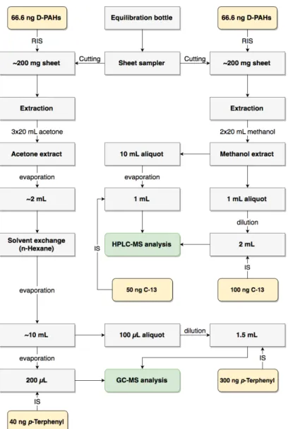
3.3.2.1 Sheet sampling and extraction ... 46
3.3.2.2 Extraction of compounds from water samples ... 47
3.3.2.3 Bottle wall sampling ... 49
3.3.3 Experiment C – Comparison of extraction methods ... 50
3.3.3.1 Speedisk® extraction method ... 51
3.3.3.2 Solvent extraction method ... 52
3.3.4 Experiment D – Direct contact method for decreasing the concentration in the polymer 53 3.3.4.1 Sample preparation ... 53
3.3.5 Experiment E – Passive sampler-water partition coefficient after direct contact method 54 3.3.6 Experiment F – Wall-water relation ... 55
3.4 Monte Carlo method for partition coefficient uncertainty estimation ... 56
3.4.1 Equation model ... 56
3.4.1.1 Passive sampler sample preparation ... 56
3.4.1.3 Calibrators ... 58
3.4.1.4 Final model equation ... 60
3.4.2 Uncertainty propagation ... 60
Chapter 4 Results and discussion ... 63
4.1 Silicone sheets comparison ... 65
4.2 Polymer-water partition coefficients ... 65
4.2.1 Equilibrium by compound release from silicone rubber to water ... 66
4.2.2 Equilibrium by compound uptake from water to silicone rubber ... 71
4.3 Sampling rate estimation ... 74
4.4 Monte Carlo method ... 76
Chapter 5 Conclusions ... 79
Literature ... 83
Annexes
A.1 GC-MS data for polymer-water partition coefficients calculations ... A-3 A.2 LC-MS data for polymer-water partition coefficients calculations ... A-6 A.3 Data used for direct contact method ... A-7 A.4 Data from temporal evolution experiment (experiment F) ... A-9 A.5 Compound distribution graphics between phases ... A-10 A.6 Direct contact method results from GC-MS analysis ... A-13 A.7 Direct contact method results from LC-MS analysis ... A-16 A.8 Sample preparation methods and techniques ... A-17
List of figures
Chapter 2 Background review
Figure 2.1 Number of peer-reviewed articles on the development and the application of passive
samplers for monitoring organic contaminants in water published between 2008 and 2017. ... 14
Figure 2.2 Main application areas of passive sampling used to monitor the quality of different
environment compartments between 2008 and 2017. ... 14
Figure 2.3 Conceptual diagram illustrating that the passive sampler detects the activity of the sampled
environment. Adapted from [60]. ... 16
Figure 2.4 Comparison of TWA concentration (dashed line) using passive sampling against spot
sampling concentrations. Adapted from [46]. ... 17
Figure 2.5 Schematic representation of the physical concentration gradient and the water turbulence
gradient established at the passive sampler-water interface at steady state. Adapted from [40]. .. 19
Figure 2.6 Differences in passive sampling and mass transfer between absorption-based and
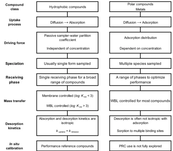
adsorption-based passive samplers. Adapted from [78]. ... 23
Figure 2.7 The two main operating regimes for passive sampling devices. Adapted from [46]. ... 25 Figure 2.8 Concentration distribution between the different layers with thickness d. Adapted from
[98]. ... 29
Figure 2.9 Uptake and release profile of a compound and a PRC, respectively, with similar Kpw, in an open system. Adapted from [29]. ... 30
Figure 2.10 Scheme of a typical GC-MS system. Adapted from [114]. ... 32 Figure 2.11 Scheme of a LC-MS system. Adapted from [114]. ... 33 Figure 2.12 Input-output model illustrating the propagation of uncertainty for three independent input
quantities X = (X1, X2, X3)T. Adapted from [125]. ... 39
Chapter 3 Experimental work
Figure 3.1 Schematic representation of experiment A sample preparation procedure. ... 45 Figure 3.2 Schematic representation of experiment B sample preparation procedure of passive
sampler samples. ... 47
Figure 3.3 Schematic representation of experiment B sample preparation procedure of water phase
samples. ... 49
Figure 3.4 Schematic representation of experiment B sample preparation procedure of bottle wall
samples. ... 50
Figure 3.5 Schematic representation of experiment C Speedisk® extraction procedure of water phase
samples for GC-MS analysis. ... 51
Figure 3.6 Schematic representation of experiment C solvent extraction procedure of water phase
samples for GC-MS analysis. ... 52
Figure 3.7 Schematic representation of the sample preparation for direct contact method experiment.
... 54
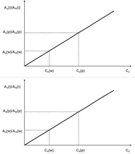
Figure 3.8 Calibration curves for the estimation of the concentration of water and passive sampler
extracts. Upper part: non-deuterated concentration related terms; Down part: deuterated
xiv
Figure 3.9 Map of all of the input quantities of the equation model. The equations red terms are
calculated from previously simulated terms. The slope and the intercept of the regression line are
estimated from all the terms involved in building the calibration curve. ... 61
Chapter 4 Results and discussion
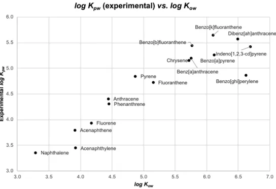
Figure 4.1 Concentration in different silicone rubber brands from silicone sheets comparison experiment. ... 65Figure 4.2 Graphical comparison between published [128] and measured log Kpw values for analysed PAHs by GC-MS. ... 68
Figure 4.3 Graphical comparison between log Kow and measured log Kpw values (by release) for analysed PAHs by GC-MS. ... 69
Figure 4.4 Graphical comparison between log Kow and measured log Kpw values (by release) for analysed PAHs and PCPs by GC-MS. PAHs #2 series excludes the three last points from PAHs series. ... 69
Figure 4.5 Graphical comparison between measured log Kpw values resulted from experiments B and C for analysed PAHs and PCPs by GC-MS. ... 70
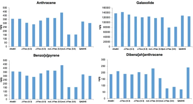
Figure 4.6 Relative amounts of selected compounds distributed between polymer, water and bottle wall. Percentages built from absolute mass (ng) values. Log Kow: Anthracene (4.45); Galaxolide (5.90); Benzo[a]pyrene (6.13); Dibenz[ah]anthracene (6.50). ... 70
Figure 4.7 Concentration levels (ng g-1) of inner and outer sheets and comparison against reference concentration for the selected compounds analysed by GC-MS (see subchapter 3.3.4 for experiment description). ... 72
Figure 4.8 Graphical comparison between log Kpw values calculated from release and uptake experiments for analysed PAHs and PCPs by GC-MS. ... 73
Figure 4.9 Graphical comparison between PCPs log Kpw values resulted from GC-MS and LC-MS analysis. ... 74
Figure 4.10 Temporal evolution of galaxolide concentration levels in the water phase and bottle wall over time. ... 75
Figure 4.11 Temporal evolution of octocrylene concentration levels in the water phase and bottle wall over time. ... 75
Figure 4.12 Modelling of octocrylene release over time. ... 76
Figure 4.13 Contribution of the various variables to the estimated uncertainty of log Kpw. ... 77
Figure 4.14 Log Kpw probability distribution function (log-normal) of phenanthrene. ... 77
Annexes
Figure A.1 Silicone polymer sheets cut-out after removal of the rod from the bottle. ... A-17 Figure A.2 Pieces of cut silicone polymer sheets in vials for solvent extraction. ... A-17 Figure A.3 Solvent extraction of silicone polymer sheets accompanied by stirring. ... A-18 Figure A.4 Resulted extract in evaporation flasks. ... A-18 Figure A.5 Kuderna-Danish evaporation system. ... A-19 Figure A.6 Extract in mini-vials after KD evaporation. ... A-19 Figure A.7 Nitrogen flow assisted evaporation system. ... A-20
Figure A.8 Sampling of the water phase from the equilibration bottles through Speedisk® by gravity.
... A-20
Figure A.9 Speedisk® water phase sampling. ... A-20 Figure A.10 Speedisk® elution to evaporation flasks. ... A-21 Figure A.11 Solvent extraction technique constituted by an extraction bottle with a phase separation
glassware. ... A-21
Figure A.12 Polymer sheets placed in glass rods inside the bottle for temporal evolution experiment
(experiment F). ... A-22
Figure A.13 Bottles in the stirrer during the exposure time regarding the temporal evolution
List of tables
Chapter 1 Introduction
Table 1.1 The 16 PAHs included in the US EPA priority pollutant list [9]. ... 4
Table 1.2 Advantages and disadvantages of direct and passive sampling [37]. ... 8
Table 3.1 Silicone rubbers used in the uptake comparison experiment. ... 44
Chapter 3 Experimental work
Table 3.2 Stepwise addition method for silicone rubber load-up. ... 46Table 3.3 Experiment B passive sampler samples listing and miscellaneous information. ... 47
Table 3.4 Experiment B water samples listing and miscellaneous information. ... 48
Table 3.5 Experiment B wall samples listing and miscellaneous information. ... 50
Table 3.6 Experiment C Speedisk® extraction samples list. ... 51
Table 3.7 Experiment C solvent extraction samples list. ... 52
Table 3.8 Sample listing for direct contact method experiment. ... 53
Table 3.9 Experiment E sample listing of passive sampler samples for analysis. ... 55
Table 3.10 Experiment E sample listing of water phase samples for analysis. ... 55
Table 3.11 Experiment F sample listing for GC-MS analysis. ... 56
Table 3.12 Summary of the preparation of calibrators 1 to 4. ... 58
Table 3.13 Summary of the preparation of calibrators 5 to 8. ... 59
Table 3.14 MS-Excel spreadsheet functions for Monte Carlo simulation [123]. ... 60
Chapter 4 Results and discussion
Table 4.1 List of selected compounds for equilibration and some of its relevant properties. ... 66Table 4.2 Silicone rubber-water partition coefficients from various equilibrations (log Kpw). ... 67
Table 4.3 Polymer-water partition coefficients (log Kpw) resulted from the set of experiments D and E. ... 73
Chapter 5 Conclusions
Table 5.1 Best estimated polymer-water partition coefficients. ... 82Annexes
Table A.1 GC-MS peak areas of samples from experiment B (subchapter 3.3.2). SD: Speedisk®
xviii
Table A.2 GC-MS peak areas of samples from experiment C (subchapter 3.3.3). SE: solvent
extraction; SD: Speedisk® extraction. ... A-4
Table A.3 GC-MS peak areas of samples from experiment E (subchapter 3.3.5). DIL: diluted samples
from extract subsampling. ... A-5
Table A.4 LC-MS peak areas of samples from experiment B (subchapter 3.3.2). CON: more
concentrated samples from extract subsampling; SD: Speedisk® extraction. ... A-6
Table A.5 LC-MS peak areas of samples from experiment E (subchapter 3.3.5). CON: more
concentrated samples from extract subsampling; DUP: duplicate. ... A-6
Table A.6 GC-MS data (in ng per vial) of samples from experiment D (subchapter 3.3.4). DIL: diluted
samples from extract subsampling; i: inner sheet; o: outer sheets. ... A-7
Table A.7 LC-MS data (in ng per vial) of samples from experiment D (subchapter 3.3.4). DIL: diluted
samples from extract subsampling; i: inner sheet; o: outer sheets. ... A-8
Symbols and abbreviations
Symbols
!"# Average of r sample readings
$#(&) Peak area of non-deuterated analyte in calibrator i
$((&) Peak area of deuterated analyte in calibrator i $)*(&) Peak area of internal standard in calibrator i
+,-#. Standard uncertainty associated with the scale calibration
+,/01 Standard uncertainty associated with weighing repeatability
+2-#. Standard uncertainty associated with volumetric material calibration
+2/01 Standard uncertainty associated with the volume measurement repeatability
+230,1 Standard uncertainty associated with the temperature effect
45**6 Volume of intermediate solution of non-deuterated analyte added for calibrators
preparation
45**7 Volume of intermediate solution of deuterated analyte added for calibrators preparation
4**6 Volume of stock solution of non-deuterated analyte added for calibrators preparation
4**7 Volume of stock solution of deuterated analyte added for calibrators preparation 4)* Volume of internal standard solution added for calibrators preparation
438. Volume of toluene added for calibrators preparation
9̅ Average of calibration standards concentrations !" Average of R readings of calibration standards ;<=> Density of water
r Density
d Dirac function
d Thickness
a Volume expansion coefficient
db Thickness of the biofilm layer
dm Thickness of the passive sampler membrane
dw Thickness of the water boundary layer
[p] Concentration of compound in the passive sampler [w] Concentration of compound in the water phase
A Area
a Half-range of a variable
a- Lower limit of an interval a+ Upper limit of an interval
xx
Aa(p) Peak area of non-deuterated analyte in the passive sampler sample Aa(w) Peak area of non-deuterated analyte in the passive sampler sample Ad(p) Peak area of deuterated analyte in the passive sampler sample Ad(w) Peak area of deuterated analyte in the passive sampler sample AIS(p) Peak area of internal standard in the passive sampler samples AIS(w) Peak area of internal standard in the water sample
b Slope
C Concentration
Ca(p) Concentration of non-deuterated analyte in the passive sampler sample Ca(w) Concentration of non-deuterated analyte in the water sample
Cd(p) Concentration of deuterated analyte in the passive sampler sample Cd(w) Concentration of deuterated analyte in the water sample
cinter Estimated concentration of the sample solution
Cmix Concentration of the D-PAHs recovery standard solution Cp Concentration of compound in the passive sampler Cstk Concentration of the D-PAHs stock solution Cw Concentration of compound in the water phase Cw,TWA TWA concentration in water
Cw0 Aqueous concentration at ? = 0
D Diffusion coefficient
d Molecular diameter
Db Diffusion coefficient in the biofilm layer
Dm Diffusion coefficient in the passive sampler membrane Dp Passive sampler material diffusion coefficient
Dw Diffusion coefficient in the water boundary layer feq Fraction of equilibrium
g Constant
Gx(x) Distribution function
gx(x) Probability density function of the value x I0 Total mass transfer resistance
Ib Mass transfer resistance of the biofilm layer
Im Mass transfer resistance of the passive sampler membrane Iw Mass transfer resistance of the water boundary layer
J Flux
k Mass transfer coefficient
kb Boltzmann constant
ke Release rate constant
km Mass transfer coefficient in the passive sampler membrane Kow Octanol-water partition coefficient
Kpm Polymer-methanol partition coefficient Kpw Polymer-water partition coefficient
ku Uptake rate constant
kw Mass transfer coefficient in the water boundary layer
L Thickness
M Number of trials
m(p) Mass of the passive sampler sample
ma(p) Mass of non-deuterated analyte in the passive sampler ma(w) Mass of non-deuterated analyte in the water phase
mdi(p) Mass of deuterated analyte spiked in the passive sampler sample mdi(w) Mass of deuterated analyte spiked in the water sample
mp Mass of the passive sampler
N Number of inputs
n Number of moles
Nmax Maximum amount of compounds that the passive sampler can handle ns Number of sheets composing the composite membrane
Nstart Amount of PRCs spiked prior to the deployment of the passive sampler Nt Amount of compound in the passive sampler after t days of exposure
q Diffusion cross-section
R Number of calibration standards readings
r Number of sample readings
Rd(p) Recuperation factor for passive sampler analysis Rd(w) Recuperation factor for water phase analysis
Rs Sampling rate
s(Y) Standard uncertainty associated with the output quantity
Sy Residual standard deviation of the calibration line
T Matrix transpose
T Temperature
t Time
t50 Time to reach half-equilibrium u Combined standard uncertainty
U Expanded combined uncertainty
u(xi) Standard uncertainty associated with a variable xi
xxii
uinter Standard uncertainty associated with the interpolation of the sample signal in the calibration line
um(u) Standard uncertainty associated with a single weighing uy Combined standard uncertainty of y
V(w) Volume of water sampled
VA Aliquot of d-phenanthrene VB Aliquot of d-naphthalene VC Aliquot of d-perylene
VD Aliquot from the intermediate solution VE Volume needed to assess the final volume VEN(p) Volume of the passive sampler sample VEN(p) Volume of the water sample
VF Volume of D-PAHs recovery standard solution spiked in the passive sampler sample VG Volume of D-PAHs recovery standard solution spiked in the water sample
Vp Passive sampler capacity
Vw Volume of water
x Diffusion path
X Vector of input quantities
xi Concentration of each i calibration standard
y Measurand
yr Output quantity of trial r
µ Dynamic viscosity
Abbreviations
D-PAH Deuterated-polycyclic aromatic hydrocarbon DBL Diffusion boundary layer
DCM Dichloromethane
DDT Dichlorodiphenyltrichloroethane DEQ Degree of equilibrium
EP European Parliament
EQS Environmental Quality Standard
EU European Union
GC Gas chromatography
GLC Gas-liquid chromatography GSC Gas-solid chromatography
GUM Guide to the Expression of Uncertainty in Measurement HOC Hydrophobic organic compound
KD Kuderna-Danish concentrator LAS Linear alkylbenzene sulfonates
LC Liquid chromatography
LDPE Low-density polyethylene LRT Long-Range Transport
LRTAP Long-Range Transboundary Air Pollution MCM Monte Carlo Method
MS Mass spectrometry
PAH Polycyclic aromatic hydrocarbon PCB Polychlorinated biphenyl
PCP Personal care product PDMS Polydimethylsiloxane
POM Polyoxymethylene
POP Persistent Organic Pollutant PRC Performance reference compound SPMD Semipermeable membrane device TWA Time weighted average
UNEP United Nations Environment Programme US EPA United States Environmental Protection Agency
UV Ultraviolet
WBL Water boundary layer WFD Water Framework Directive
Chapter 1
Introduction
Introduction
We rely on access to clean, safe water for consumption and utility in all aspects of our societal activities. Though, water is also a transport medium carrying away the byproducts of our settlements and dispersing them into the environment. As population and settlements grew larger, new types of waste produced became increasingly alien to the natural environment, and the problem of water pollution with endemic environmental degradation also became obvious. It is therefore of greatest importance to preserve and safeguard the remaining water resources, and to ensure their sustainable management. So, environmental monitoring of water is becoming increasingly important. Policy programs on water management have being adopted by authorities around the globe with ambitious goals and approaches that can be used for preserving quality of water.
1.1 Persistent organic pollutants
Persistent organic pollutants (POPs) are ubiquitous chemical contaminants that persist in the environment for long periods after their release and bioaccumulate heavily in the food chain, mainly in fatty tissues, reaching concentrations capable of having harmful effects on human health and on the environment [1-3]. In addition to this, POPs can potentially be transported over great distances and dispersed around the globe by air and ocean currents. They therefore pose a risk to the environment and human health not only locally and regionally, but also in parts of the world at a great distance from the point of emission [4, 5]. POPs are characterized by low aqueous solubilities, low vapor pressures, lipophilic properties, and extended half-lives in environmental media. There is, unsurprisingly, concern regarding the presence of POPs in the environment and the potential impact on human health and ecosystems balance due to their toxicity, carcinogenicity, mutagenicity, and teratogenicity. Human exposure to POPs may result from a variety of pathways including inhalation of contaminated dust and particulate matter, oral ingestion, or dermal absorption [3].
The concern around the presence of POPs in the environment has led to the adoption of an international treaty in 2001, the Stockholm Convention on POPs, intended at restricting and ultimately eliminating the release of POPs to the environment [3, 6]. Initially, 12 POPs were targeted, including pesticides, industrial chemicals like PCBs, and by-products such as dioxins and furans. Although not included in the list of restricted compounds, polycyclic aromatic hydrocarbons (PAHs) represent another class of POPs that have the potential to cause adverse effects on ecosystem and human health [3, 7].
1.1.1 Polycyclic aromatic hydrocarbons
Polycyclic aromatic hydrocarbons (PAHs) are a group of organic compounds consisting of molecules containing two or more fused benzene rings, although bicyclic compounds sometimes are included in the term. When a pair of carbon atoms is shared, then the two sharing aromatic rings are considered fused. The resulting structure is a molecule where all carbon and hydrogen atoms lie in one plane [8, 9]. These compounds are toxic, and they bioaccumulate, especially in invertebrates in the aquatic environment. Despite vertebrates can metabolize PAHs, their metabolites are reactive compounds and some of those are carcinogenic as well. The environmentally significant PAHs range between naphthalene and coronene. In this range, there is a large number of PAHs, differing in the number and position of aromatic rings, with varying number, position and eventual chemical substituents on the basic ring system. Physicochemical properties of PAHs vary with molar mass [10], and they are included in the US EPA and in the European Union priority lists of pollutants due to the environmental concern around these group of compounds. US EPA has identified sixteen unsubstituted PAHs as priority pollutants, some of which are considered to be possible or probable human carcinogens, and hence their
Chapter 1
4
distribution in the environment and potential risks to human health have being the focus of much attention. The sixteen US EPA PAHs along with their structures and physicochemical constants are given in Table 1.1.
Table 1.1 The 16 PAHs included in the US EPA priority pollutant list [11].
PAHs are introduced into the environment mainly via natural and anthropogenic combustion processes. Important anthropogenic sources include combustion of fossil fuels, oil refining, incomplete combustion of organic material, aluminum and coke and asphalt production and many other industrial activities [12]. From combustion processes PAHs are emitted to the air when no abatement systems are in place. In general, all thermal processes containing carbon and hydrogen are potential sources of PAHs. The formation of PAHs from these processes are closely correlated to the processes conditions, and the quantity emitted depends on the applied abatement system.
PAHs are spread to the marine environment by both atmospheric and aquatic pathways. They can reach water bodies mainly through dry and wet deposition, road runoff, industrial wastewater, and leaching from creosote-impregnated wood [13-17]. After entering the aquatic environment, the behavior and fate of PAHs depend on their physicochemical properties. Volatilization, dissolution, adsorption onto
Introduction
suspended solids and subsequent sedimentation, biotic and abiotic degradation, uptake by aquatic organisms and accumulation, are all major processes to which PAHs in water are subject [8, 9].
1.1.2 Personal care products
Personal care products (PCPs) have received growing attention in recent years as emerging contaminants due to their potential threats to aquatic environment and human health. They are a diverse group of organic compounds and integrate of daily personal care products such as soaps, lotions, toothpaste, fragrances, sunscreens, to name a few. The primary classes include disinfectants, fragrances, insect repellants, preservatives and UV filters [18, 19]. PCPs are widely used in high quantities throughout the world, and since they are intended for external use, they are not subjected to metabolic alterations. Therefore, large quantities of PCPs enter the environment unaltered through regular use [20]. Some studies have indicated that many PCPs are environmentally persistent, bioactive, and have the potential for bioaccumulation [21, 22]. While not all PCPs are persistent, their continuous use and release to the environment means many are considered “pseudo-persistent”. This suggest that they have greater potential for environmental persistence because their source emission sources continually replenish, unlike other organic contaminants like pesticides [23]. Persistent exposure by PCPs can be significant even at low concentration levels [19].
PCPs are among the most commonly detected compounds in surface waters throughout the world [21]. So, there has being increasing awareness of the unintentional presence of PCPs in various compartments of the aquatic environment at concentrations capable of causing adverse effects to aquatic organisms. The continuous use of PCPs and release to the environment resulted in the identification of some of these compounds as future emerging priority candidates, in 2007. Some have even been proposed to integrate the list of priority substances as musks and triclosan were identified as future emerging priority candidates under the EU Water Framework Directive (WFD) 2000/60/EC [23].
1.2 Environmental conventions and directives
1.2.1 Water Framework Directive
In 2000, the European Parliament’s (EP) and Council’s conciliation committee finally reached an agreement on the proposed Framework Directive for Community action in the field of Water (WFD). Building on the achievements of existing EU water legislation in 2000, the WFD introduced new and ambitious objectives to protect aquatic ecosystems in a more holistic way, while considering the use of water for life and human development.
Water is the sector with the most comprehensive coverage in EU environmental regulation. EU water directives have effected considerable changes in national legislative statutes even in the countries with the most developed environmental regulation. The WFD sets common approaches and goals for the management of water in 27 countries and a number of new accession countries. The overall goal is a good and non-deteriorating status for all waters through planning at a hydrologic level and implementation of a number of pollution-control measures [24]. The WFD marked the beginning of a new era in EU environmental policy by providing guidance to MS on how to achieve and maintain good quality of waters and how the various aspects of the WFD should be reported to the European Commission [25].
Chapter 1
6
Article 16 of the Water Framework Directive sets out the strategy against chemical pollution of surface waterbodies. The chemical status assessment is used alongside the ecological status assessment to determine the overall quality of a waterbody. Environmental Quality Standards (EQSs) are key tools used for assessing and classifying the chemical status and can therefore affect the overall classification of a waterbody under the WFD. The European EQS Directive (2013/39/EU) establishes the maximum acceptable concentration and annual average concentration for 45 priority substances (Annex I) which, if met, allows the chemical status of the waterbody to be described as “good”. The current list of priority substances includes some PAHs, however PCPs are not regulated by the WFD at European level. In addition, the WFD (Annex V, section 1.2.6) establishes the principles to be applied by the MS to develop EQSs for river basin specific pollutants that are discharged in significant quantities [26]. To determine whether water bodies are of good status and what measures need to be included in order to reach good status precise and reliable monitoring results are needed, playing therefore a key role for sound planning of measurement programs. Article 8.1 of the WFD requires member states to establish monitoring programs for the assessment of the status of surface water and of groundwater in order to provide a coherent and comprehensive overview of water status. Directive 2009/90/EC on the quality and comparability of chemical monitoring specifies minimum performance criteria for methods of analysis applied by member states when monitoring water status, sediments, and biota, to ensure the quality of the analytical results [25].
1.2.2 Stockholm Convention
Detection and analysis of bioavailable pollutants at very low concentrations and investigation of the environmental concentration of organic and inorganic pollutants are being made not only on the local scale but also on continental and global scales. This issue concerns the environmental long-range transport (LRT) of organic chemicals problem, identified in the 1970s by the presence of organochlorine compounds, such as dichlorodiphenyltrichloroethane (DDT) or polychlorinated byphenils (PCBs) at remote regions, including the Arctic and Antarctic [4, 27-29]. Despite it has been well known in the 1970s, only in the 1990s this topic has received considerable attention due to the increasing scientific knowledge about organic chemicals transported to the Artic that became available in the late 1980s. Then, in the 1990s, the issue regarding LRT of organic chemicals was addressed within the framework of the Long-Range Transboundary Air Pollution (LRTAP) by the development of the 1998 Protocol on Persistent Organic Pollutants (POPs), known as the Aarhus Protocol on POPs. Also motivated by the concern about LRT of persistent organic chemicals, the beginning for a second international agreement addressing the LRT of organic chemicals was established in the 1990s. This is the Stockholm Convention on Persistent Organic Pollutants which came into force in 2004.
The Stockholm Convention has the objective of ensuring human health and the environment are protected from POPs, and any action take intended to reducing and eliminating their release is informed by the precautionary approach. To this end, different levels of regulation are laid down for the various substances it covers. It is the global treaty under the United Nation Environment Programme (UNEP) with the participation of 172 countries, and in context of this convention and the global monitoring programs, there is an increased need for development of new sampling tools that enable reliable measurement of POPs for the assessment of their spatial and temporal pollution trends [2, 5, 30-32]. Furthermore, the convention stipulates how stockpiles of the substances individually, in mixtures or in articles are to be dealt with. It requires that provisions be put in place concerning the transport of substances and their management as wastes.
Introduction
As a party to the Stockholm Convention, the EU has committed itself to implement the requirements of this international agreement. They are addressed within the framework laid down by POPs Regulation. In implementing the Stockholm Convention on Persistent Organic Pollutants, the parties to the Convention commit to take appropriate measures to prevent the release of these substances into the environment or at least reduce such releases as far as is technically feasible and economically acceptable [5].
1.2.3 OSPAR Convention
The 1992 OSPAR Convention is the current legal instrument guiding international co-operation on the protection of the marine environment of the North-East Atlantic. It combines and updates the 1972 Oslo Convention on dumping waste at sea and the 1974 Paris Convention on land-based sources of marine pollution. The work under the convention is managed by OSPAR Commission, made up of representatives of the Governments of 15 Contracting Parties and the European Commission, representing the European Community. The work applies the ecosystem approach to the management of human activities and is guided by the following thematic strategies: protection and conservation of marine biodiversity and ecosystems; eutrophication; hazardous substances; offshore oil and gas industry; radioactive substances; and monitoring assessment. Under each theme, work is undertaken in relation to the monitoring and assessment of the status of the marine environment, the results of which are used to follow up implementation of the strategies and the resulting benefits to the marine environment [33].
Since 2010, OSPAR has been working with other Regional Seas Conventions and the European Commission to develop assessment tools, such as indicators of the state of the marine environment. Measures at OSPAR, EU and international level had contributed to decreasing pressures from chemical pollution over the past 20 years. A third of OSPAR’s 26 groups of chemicals which pose a risk to the marine environment are expected have been phased out by 2020. OSPAR, while working in partnership with EU, has identified threats from a wide range of substances of possible concern for the marine environment which need to be tackled by the appropriate forum, and continues to focus on substances posing risks to the marine environment that are not yet adequately covered by the EU and to actively generate input to the EU on the identification, selection, and prioritization of hazardous substances which are of concern for the marine environment [34].
1.3 Water quality monitoring
A wide range of methods and instruments can be used for sampling and analysis of pollutants present in the environment. Nowadays, the techniques used to monitor environmental pollutants should enable not only direct monitoring the concentration of chemical pollutants but also allow evaluation of their effects and assessment of the risk for aquatic organisms and human health. Estimation of biological exposure to toxic and genotoxic environmental pollutants is a fundamental aspect of biological hazard assessment [35, 36]. Generally, assessment of the risk of pollutants is based on the concentrations determined by analytical chemistry and on toxicity and genotoxicity data of the pollutants [37]. Protection against the harmful effects of environmental pollutants requires their levels to be carefully measured. This means that in order to establish the quality of the different compartments of our environment, a large number of samples have to be taken to determine daily, monthly, and annual time-weighted average concentrations of the pollutants of interest. Based on those results further conclusions can be drawn and, moreover, prevention and improvement can be performed. As a result, long-term and
Chapter 1
8
much potential as a low-tech and cost-effective monitoring tool, avoiding almost every disadvantage of active sampling and/or sample preparation techniques. It is especially important for multipoint sampling over large and remote areas. In most cases, passive sampling vastly simplifies sample collection and preparation by elimination of electric power requirements, significant reduction of analysis costs and protection of analytes against decomposition during transport, storage, and enrichment [38], and reflects freely dissolved concentration in water. It was observed in a wide range of studies that bioaccumulation and toxicity of hydrophobic organic compounds are controlled by freely dissolved concentrations rather than by total concentrations that include bond forms [39]. Additionally, passive sampling has the advantage of collecting time integrated samples which may be more representative of predominant water concentrations when compared with direct sampling. The major disadvantage though lies on its complexity [40] and it requires further planning and experience. Table 1.2 highlights some advantages and drawbacks.
Introduction
Passive sampling has been widely accepted throughout the world for environmental sampling, as evidenced by many regulatory guidelines, manuals, and protocols published by various environmental and standards introducing authorities throughout the world [38, 41, 42].
Chapter 2
Background review
Background review
2.1 Conventional sampling
Conventional sampling is currently the major set of sampling techniques for monitoring water quality in compliance with regulatory provisions, and it is based on chemical analysis of spot samples of water taken at defined points and frequency [43, 44]. This approach is associated with a number of disadvantages that can make the determination of organic compounds erroneous. When taking a grab sample, its composition may alter at any time during sampling, transportation, preservation, storage and work-up procedures associated with contamination and analyte loss, and while the magnitude of this perturbation may be minimized, it cannot be eliminated completely. In addition, spot samples provide only instantaneous data. Thus, when monitoring for regulatory purposes the use of occasional grab sampling may result in a non-representative estimate of the pollution load status of the water bodies due to temporal and spatial variability. If the analyte concentration fluctuates, grab sampling may either miss recurring pollution episodes, and therefore underestimate the total pollution load, or catch a pollution episode as it occurs, and possibly overestimate the total pollution load. To address the problem with fluctuating pollutant levels, frequent grab sampling can be used where sampling interval is sufficiently short as to detect sporadic events. This is common solved by using automated sampling. This does not, however, address the other drawbacks related to grab sampling outlines above. Further, the laboratory methods commonly used for the analysis of spot samples of water are often not sensitive enough to fulfil the required minimum performance criteria associated with the current environmental quality standards for many priority pollutants and demonstrate reduced reproducibility with decreasing concentrations of organic pollutants in water samples [44]. This questions the fitness for purpose of traditional sampling in regulatory environmental management.
An alternative approach to measure pollutants in water is provided by the introduction of passive sampling. This technology measure time weighted average (TWA) concentrations over periods of weeks, and it has been gaining acceptance for use in regulatory environmental monitoring [44]. For organic pollutants priority pollutants, spot sampling provides total concentrations whereas passive sampling measures only the freely dissolved fraction of the compounds. This approach is especially useful in water bodies where concentrations fluctuate in time, providing more reliable routine monitoring data.
2.2 Passive sampling
Passive sampling devices are environmental monitoring tools that have been developed to facilitate the assessment of chemical pollutants concentrations in different environmental mediums, for example air, water, and soil, from the mass of targeted analytes absorbed within a receiving phase [41, 45-48]. Such devices have been extensively employed by industry for monitoring air quality since the early 1970s in order to measure toxic chemicals in workplace air.
Later the principles of passive dosimetry were brought to bear in monitoring of aqueous environments. Passive sampling methods have shown much promise as tools for measuring aqueous concentration of a wide range of priority pollutants due to their many significant advantages, including simplicity regarding handling and deployment, low cost analysis, no power requirement, unattended operation, and the ability to produce accurate results since passive samplers collect the target analyte in situ and without affecting the bulk solution [38, 49].
Passive sampling is still a technology under development though, and in the last decade remarkable progress has been made in passive devices design, calibration methods, and quality assurance. A large
Chapter 2
14
and yet still growing number of publications dedicated to this technology proves its large potential and testifies to its utilization for environment monitoring. Figure 2.1 proves that the interest in passive technology has grown over the last ten years as it presents the number of peer-reviewed publications during that time regarding the application of passive sampling technology for water monitoring pollutants only [46, 49, 50-53]. The search was done employing the Scopus database of peer-reviewed literature applying passive, sampling and water key-words [54].
Figure 2.1 Number of peer-reviewed articles on the development and the application of passive samplers for
monitoring organic contaminants in water published between 2008 and 2017.
Since its first deployment in air quality assessment, the application of passive sampling techniques had spread to other research areas. Environmental Sciences are unquestionably the predominating areas of passive sampling application particularly in water compartment monitoring [38, 55-58]. Approximately 47% of the total number of publications in the last ten years (from 2008 to 2017) describes the use of passive samplers to monitor water environmental quality conditions, as it is shown in Figure 2.2 [54].
Figure 2.2 Main environmental compartments monitored by passive sampling between 2008 and 2017.
A few new applications can be observed, however. In general, passive sampling has been mostly applied for [38]:
§ Screening studies and source identification – determination of occurrence or
identification of pollutants in a given environmental compartment;
0 30 60 90 120 150 2008 2009 2010 2011 2012 2013 2014 2015 2016 2017 Nu m b er o f p u sb lis h p ap er s Water 45% Sediment 7% Ground water 2% Air 36% Soil 10%
Background review
§ Determination of the pollutant concentrations in the environment – integration of
ambient concentrations of ambient concentrations of pollutants over time scales;
§ Mapping the ambient distribution of pollutants to support national and international
monitoring networks – spatial distribution of pollution levels in the form of maps;
§ Studying changes in pollutant concentrations and composition along environmental
gradients;
§ Human exposure assessment;
§ Determination of concentrations of environmental pollutants by equilibrium
sampling;
§ Water quality monitoring;
§ Bio-availability of contaminants in sediments;
§ Bioanalytical assessment – determination of bioaccumulation levels of pollutants in
biological samples;
§ Ecotoxicology testing – collection of material for toxicity tests.
Regarding the use of passive sampling to assess the quality of the environment, research is continuously been conducted to enable better understanding of kinetic uptake and sampling rates of passive samplers and better understanding of samplers’ performance.
2.2.1 Passive sampling principles
Passive sampling is a technology that is based on the free flow of analyte molecules from sample matrix to the receiving phase. The devices used for passive sampling consists on diffusion through a diffusion barrier or permeation through a membrane [49-51, 59]. Diffusion driving forces and separation mechanisms are an outcome of the different concentration, pressure, temperature, and electromotive force gradients, which can be reduced to fundamental chemical potential gradients, of the analyte between the two media resulting in the enrichment and isolation of analytes onto the receiving phase [49, 60, 61]. The receiving phase of a passive sampler can be solvent, polymer, chemical reagent or porous adsorbent [61]. The affinity of chemicals to the sampling material depends on the strength of interactions such as van der Waals interactions and hydrogen bonding [62].
These contaminants of concern concentrations are frequently so low that they are not detectable with the existing analytical techniques unless very large volumes of water are extracted. The passive sampling system overcomes this problem by reason of the sampler device having a small volume, but a very high uptake capacity for the analyte. The uptake capacity of a sampler, expressed as an equivalent maximum sampled volume of water, can be expressed by equation 2.1:
41 = B1C ∙ F1 (2.1)
where Vp (L) is the sampler’s uptake capacity, Kpw (L×kg-1) is the compound’s partition coefficient between the sampler and the water medium, and mp (kg) is the sampler’s mass. Common contaminants like polychlorinated biphenyls (PCBs) and polycyclic aromatic hydrocarbons (PAHs) are hydrophobic,
Chapter 2
16
therefore passive sampling takes advantage of the hydrophobicity of these contaminants to collect and concentrate them by deploying material in the system been assessed or monitored that is also hydrophobic, like organic polymer-based passive samplers. If a hydrophobic material is placed into water, hydrophobic contaminants will partition from water into the passive sampler. The greater the affinity of a given contaminant to the sampler material the greater is the partition coefficient between the sampler material and aquatic medium, and the greater is the capacity of the sampler for that particular contaminant.
When a passive sampler is deployed in water with contaminants, such as PCBs and PAHs, present in the dissolved phase, they will partition into the sampler. Over time, contaminants will accumulate in the sampler until the contaminants are considered to be at equilibrium between the passive sampler and the various environmental phases. At thermodynamic equilibrium, the chemical activity across environmental compartments is by definition equal, and freely dissolved concentration is directly related to the concentration in the passive sampler polymer phase (figure 2.3). Thus, while the mass of compounds in different phases may vary depending on the phase uptake capacity of the phases, the activity across phases is constant [63]. Equilibrium is established when the change in the amount of contaminants transferring from one phase to another is no longer significant. Though it can be an abstract concept, equilibrium simply indicates that we do not expect any significant change over time in the concentration of a given contaminant in any phase we may want to measure. A clear way to visualize equilibration for contaminants concentrations is to plot concentration versus time.
.
Figure 2.3 Conceptual diagram illustrating that the passive sampler detects the activity of the sampled
environment. Adapted from [63].
Once the concentration in the sampler is no longer changing with time, we can conclude that equilibrium has been achieved [64]. Equilibrium can also be predicted if the partition coefficient between the sampler and the water medium for a given contaminant, and the passive sampler uptake rate are known. The equilibrium times of a passive sampler for different compounds range from a few days to months. The determination of freely dissolved fraction of contaminants in water is an important feature of passive sampling technique especially for organism exposure and bioavailability assessment [65]. Though, contaminants may be associated with several environmental phases in water and not all are equally bioaccessible or bioavailable. Contaminants truly dissolved in water are considered very bioaccessible and therefore likely to be bioavailable and taken up by an organism. It is critical to note that contaminants freely dissolved in the water are not the only bioavailable contaminants in an environmental system. Other phases can contribute bioavailable concentration in a given environmental system. Understanding environmental phases and where a contaminant resides in these phases can assist
Background review
in establishing whether the contaminants will be in a form resulting in exposure to aquatic organisms, wildlife and humans.
Passive samplers collect contaminants only from the bioaccessible form and thus are good estimators of what is bioavailable [39, 64, 66]. The passive samplers are time-integrative samplers because they typically integrate the concentrations of analytes over the whole exposure time (when a passive sampler remains far from equilibrium) making such a method less bias-prone to fluctuation of pollutant concentrations, providing the uptake capacity is so large that equilibrium with the sampled phase is not established [62, 65]. Knowing the long-term average concentrations is critical when we want to understand what local organisms are being exposed to over longer time periods. The more representative time-integrated measurement that passive samplers provide better reflects the average exposures experienced by organisms. Figure 2.4 shows the dissolved water column concentration of a hydrophobic contaminant as the actual concentration and the passive sampler-based concentration.
Figure 2.4 Comparison of TWA concentration (dashed line) using passive sampling against spot sampling
concentrations. Adapted from [49].
2.2.1.1 Laws of diffusion
Diffusion is the spontaneous molecular transport of a substance in gaseous, liquid or solid media. The forces behind this substance transport are differences in concentration, partial pressure and temperature. In general, diffusion is understood to be the process whereby molecules spontaneously migrate within a system as a result in differences in potential [67]. During passive sampling the only force behind the transport of a substance is the difference in chemical activity of that particular substance in the surrounding medium and that on the collection phase. The diffusion process can be described mathematically by Fick’s first law of diffusion (Equation 2.2):
J = −L ∙MN
M9 (2.2) where J is the flux (mol×m-2×s-1), D is the diffusion coefficient (m2×s-1), C is the concentration, the dimension of which is amount of substance per unit volume (mol×m-3), and x is the diffusion path, represented in length units (m). Fick’s first law relates diffusive flux to the concentration assuming that the transport of the substance takes place without any apparent flow, that is without movement of the whole medium. It postulates that the flux goes from region of high concentration to regions of low
![Figure 2.7 The two main operating regimes for passive sampling devices. Adapted from [49]](https://thumb-eu.123doks.com/thumbv2/123dok_br/19186085.947625/49.892.214.678.853.1109/figure-main-operating-regimes-passive-sampling-devices-adapted.webp)


![Figure 4.2 Graphical comparison between published [131] and measured log K pw values for analysed PAHs by GC-MS](https://thumb-eu.123doks.com/thumbv2/123dok_br/19186085.947625/92.892.178.726.112.480/figure-graphical-comparison-published-measured-values-analysed-pahs.webp)