THERMAL PERFORMANCE OF FIRE PROTECTION MATERIALS

(1)

THERMAL PERFORMANCE OF FIRE PROTECTION

MATERIALS

Zourkane Abdelkader

Final thesis submitted to the

School of Technology and Management

Polytechnic Institute of Bragança

For the fulfilment of the requirements for a Master’s Degree in

Industrial Engineering

Mechanical Engineering Branch

(2)

(3)

THERMAL PERFORMANCE OF FIRE

PROTECTION MATERIALS

Zourkane Abdelkader

Final thesis submitted to the

School of Technology and Management

Polytechnic Institute of Bragança

For the fulfilment of the requirements for a Master’s Degree in

Industrial Engineering

Mechanical Engineering Branch

Supervisor at IPB:

Prof Dr. Luis Mesquita

Supervisor at UHBC:

Dr. Abdellah Benarous

(4)

(5)

Thermal performance of fire protection materials

ACKNOWLEDGEMENTS:

I would like to express my gratitude and appreciation to Professors Luis Mesquita and Abdellah Benarous for their excellent guidance, supervision, dedication and support throughout this year. The advices and comments of both professors that have been a considerable help and of great value for the successful and conclusion of this work.

Special thanks go to my family and friends for their continuous support and patience. I would like to thank the Erasmus + ICM, Internship and double diploma award between the

Polytechnic Institute of Braganҫa (IPB) and the University Hassiba ben Bouali de Chlef

(UHBC).

Thank you for your helpful technical advice, your support and encouragement during this period, for your cheerfulness, patience and love; thank you for always being at my side. Fruitful result would not hasten without the moral support and encouragement of my family, my lovely and beautiful mother Lalia, my father Ahmed, my brothers Taher and Moussa and my sisters Aicha and Hadjer, that have enabled me to achieve this today.

Friendship is a wonderful blessing from God, I am blessed with my friends Thabet Ridha, Rami, Mohamed, Billel, Houssin, Soufyane, Hakima, Sabrina, Habib, Djilali, Hakim, Amhamed, Khaled, Belkacem, Jhony Lima, Hasmik, Seddik, Yassin, Younes, Youssef, Yasser, Abdelrahman, benouda, Amin, Khalil, Remdan, Lid, Nasser, Meloud, Howari, Aboubakr, Saif dean, Ferdous and Khaled for their moral support and encouragement, I am so glad to share this experience with you.

(6)

(7)

Resumo

O método mais comum de se obter a resistência ao fogo requerida é através do uso de sistemas passivos de proteção contra fogo, nos quais o material mais utilizado são as placas de silicato de cálcio.

A utilização do Eurocódigo 3 parte 1.2 para a evolução da temperatura do aço dos elementos protegidos contra o fogo requer o conhecimento das propriedades térmicas dos materiais aplicados em função da temperatura. Normalmente, estas propriedades não são conhecidas para todos os materiais e nem para toda a gama de temperaturas necessárias na verificação de segurança ao fogo.

O objetivo deste trabalho é desenvolver um conjunto de testes experimentais realizados com o objetivo de caraterizar a eficiência térmica durante a sua exposição a temperaturas elevadas. Os testes são conduzidos num calorímetro de cone usando diferentes espessuras de placas de aço e espessuras de placas de isolamento e fluxos de calor por radiação. Os resultados dos testes experimentais são comparados com os obtidos a partir de resultados numéricos usando o método de diferenças finitas, implementado em Matlab. Uma atenção particular é dedicada à modelação numérica das reações químicas e da evaporação da água devidas ao aumento da temperatura do material de isolamento, placas de silicato de cálcio.

Os resultados mostram a comparação entre as temperaturas medidas na chapa de aço carbono expostas a temperatutras elevadas e as temperaturas obtidas pelo método simplificado do Eurocódigo e pelo modelo numérico, seguem a mesma tendência. A diminuição da temperatura do aço ocorre com o aumento da espessura da placa de aço carbono, do fluxo de calor e com o aumento da espessura das placas de isolamento.

Palavras-chave:

(8)

(9)

Abstract

The most common method of achieving the required fire resistance is by the use of passive fire protection systems, in which the most common material calcium silicate board is used.

The use of the Eurocode 3 part 1.2 for the steel temperature evolution of fire protected elements require the knowledge of the thermal properties of the applied materials in function of the temperature. Usually these properties are not known for all the materials and not for all the temperature range needed for fire design.

The aim of this work is to develop an experimental set of tests made with a fire insulation material in order to characterize the thermal efficiency during the temperature exposure. Tests are made in a cone calorimeter using different steel plate thickness, insulation plate thickness and radiative heat fluxes. The experimental tests results are compared with the one obtained from numerical results using the finite difference method by implementing in Matlab. Special care is made to include the chemical reactions and evaporation of water from the heating of the insulation material, calcium silicate boards.

Results showed the comparison between the measured temperatures in carbon steel plate exposed to fire and the corresponding calculated temperatures presented a very good agreement and the decrease in the temperature vary with the increase of the thickness of carbon steel plate and heat flux and the fire insulation boards.

Keywords:

(10)

(11)

INDEX

ACKNOWLEDGEMENTS: ... I

RESUMO ... III

ABSTRACT ... V

INDEX ... VII

LIST OF FIGURES ... IX

LIST OF TABLES ... XIII

SYMBOLOGY ... XV

CHAPTER 1: MOTIVATION AND OUTLINE ... 1

1.1 MOTIVATION ... 1

1.2 OBJECTIVE ... 1

1.3 OUTLINE ... 2

CHAPTER 2: STATE OF THE ART ... 3

CHAPTER 3: SIMPLE METHOD OF EUROCODE ... 7

3.1 INTRODUCTION ... 7

3.2 STEEL TEMPERATURE DEVELOPMENT UNPROTECTED INTERNAL STEELWORK ... 7

3.3 NUMERICAL RESULT ... 10

CHAPTER 4: CONE CALORIMETER EXPERIMENTAL TESTS ... 14

4.2 PREPARATION OF THE SPECIMENS ... 15

4.3 CALIBRATION OF THE CONE CALORIMETER: ... 16

4.4 EXPERIMENTAL TESTS FOR UNPROTECTED STEEL: ... 17

4.5 EXPERIMENTAL TESTS FOR PROTECTED STEEL: ... 20

4.6 EXPERIMENTAL TESTS FOR PROTECTED STEEL ... 21

4.7 COMPARISON BETWEEN THE UNPROTECTED AND PROTECTED CARBON STEEL PLATE ... 25

(12)

CHAPTER 5: THE HEAT TRANFER EQUATION BY THE FINITE DIFFERENCE

METHOD 29

5.2 STEEL AND INSULATION ENERGY EQUATION ... 29

5.3 THE FINITE DIFFERENCE METHOD ... 34

5.4 METHOD OF LINES ... 35

5.5 COMPARISON BETWEEN EXPERIMENTAL AND NUMERICAL RESULTS OF UNPROTECTED STEE37 5.1 COMPARISON BETWEEN EXPERIMENTAL AND NUMERICAL RESULT OF PROTECTED STEEL .... 42

CHAPTER 6: CONCLUSIONS AND FUTURE WORK ... 52

6.1 MAIN CONCLUSIONS ... 52

6.2 FUTURE LINES OF INVESTIGATION ... 53

REFERENCES ... 54

(13)

LIST OF FIGURES

Figure 1: Specific heat of carbon steel as a function of the temperature, [8]. ... 9

Figure 2 : The temperature variation with time for ISO834 and unprotected steel plate. .. 10

Figure 3 : The temperature variation with time for ISO834 and protected steel plate, ds=5. ... 11

Figure 4 : The temperature variation with time for ISO834 and protected steel plate, ds=7.5. ... 12

Figure 5 : The temperature variation with time for ISO834 and protected steel plate, ds=10. ... 12

Figure 6: Picture of the Cone Calorimeter... 14

Figure 7: The materials used. ... 15

Figure 8: The specimen of the unprotected carbon steel plate prepared. ... 16

Figure 9 -: Programme MLCCalc to calibrate the cone calorimeter. ... 16

Figure 10: Schematic drawing of apparatus, [12]... 17

Figure 11: Cone calorimeter and experimental setup. ... 17

Figure 12: The temperature variation with time for the 3.6 [mm] thickness plate. ... 18

Figure 13: The temperature variation with time for the 7.75 [mm] thickness plate. ... 18

Figure 14: The temperature variation with time for the 14 [mm] thickness plate. ... 19

Figure 15: The specimen of the protected carbon steel plate prepared. ... 20

Figure 16: Cone calorimeter and experimental setup. ... 21

Figure 17: The temperature variation with time for the 3.6 [mm] thickness plate and dp 15 [mm]. ... 21

(14)

Figure 20: The temperature variation with time for the 3.6 [mm] plate and dp 20 [mm]. .. 23

Figure 22: The temperature variation with time for the 14 [mm] thickness plate and dp 20 [mm]. ... 24

Figure 23: The temperature variation with time for unprotected and protected steel plate with insulation of 15 [mm] thickness. ... 25

Figure 24: The temperature variation with time for unprotected and protected steel plate dp=20 [mm] thickness. ... 26

Figure 25 : Mass loss after 24 h at 100 [°c]. ... 27

Figure 26 : schematic drawing for specimen ... 30

Figure 27: Triangular variation of specific heat during moisture evaporation. ... 33

Figure 28: Finite Difference discretization of a function u or T. ... 34

Figure 29: Results of the numerical method and experimental with thickness ds=3.6[mm] and heat flux q=35[KW/m²]. ... 38

Figure 32: Results of the numerical method and experimental with thickness ds=7.75[mm] and heat flux q=35 [KW/m²]. ... 39

Figure 33: Results of the numerical method and experimental with thickness ds=7.75[mm] and heat flux q=50 [KW/m²]. ... 39

Figure 34: Results of the numerical method and experimental with thickness ds=7.75[mm] and heat flux q=75[kw/m²]. ... 40

Figure 35: Results of the numerical method and experimental with thickness ds=14[mm] and heat flux q=35[kw/m²]. ... 40

Figure 38: Parametric analysis of the moisture evaporation. ... 43

(15)

Figure 40: The experimental result and numerical result of protected carbon steel plate ds=3.6 [mm] with insulation dp=15 [mm] thickness. ... 45 Figure 41: The experimental result and numerical result of protected carbon steel plate

ds=7.75 [mm] with insulation dp=15 [mm] thickness. ... 45 Figure 42: The experimental result and numerical result of protected carbon steel plate

ds=14 [mm] with insulation dp=15 [mm] thickness. ... 46 Figure 43: The experimental and numerical result of protected carbon steel plate with

ds=3.6 [mm], dp=20 [mm] and q=35 [kw/m²]. ... 48 Figure 44: The experimental and numerical result of protected carbon steel plate with

ds=3.6[mm], dp=20 [mm] and q=50 [kw/m²]. ... 48 Figure 45: The experimental and numerical result of protected carbon steel plate with

ds=14 [mm], dp=20 [mm] and q=35 [kw/m²]. ... 50 Figure 50: The experimental and numerical result of protected carbon steel plate with

ds=14 [mm], dp=20 [mm] and q=50 [kw/m²]. ... 50 Figure 51: The experimental and numerical result of protected carbon steel plate with

(16)

(17)

LIST OF TABLES

Table 1 - Recent publications on insulation materials ... 3

Table 2 - Results of protected and unprotected steel in Matlab. ... 13

Table 3 - Results of experimental test of unprotected steel plate. ... 19

Table 4 - Results of experimental test of protected steel dp=15[mm]. ... 23

Table 5 - Results of experimental test of protected steel dp=20[mm]. ... 24

Table 6 – Mass loss of calcium silicate board with different thickness. ... 28

Table 7 – The result of temperature between experimental and numerical result for unprotected steel plate. ... 41

Table 8 - Thermal Conductivity and Heat Capacity of Mild Steel vs. Temperature, [13]. . 42

Table 9 – Thermal properties of Promatect-200, [10]. ... 43

Table 10 - Thermal properties of Promatect-H, [19]. ... 43

Table 11 - The result of temperature between experimental and numerical result for protected steel plate with dp =15 [mm]. ... 47

(18)

(19)

SYMBOLOGY

LATIN UPPERCASE LETTERS

Am /V is the section factor

Ap is the appropriate area of fire protection material per unit length of the member

[m²]

Ksh is the correction factor for shadow effect

N is the number of grid points T is the temperature

Tg is the gas temperature in the vicinity of the fire exposed member

Ts is the surface temperature of the member

UNP is the unprotected steel plate XL is the left boundary condition

XR is the right boundary condition

LATIN LOWERCASE LETTERS

a

c

is the specific heat of steel

p

(20)

dp is the thickness of fire protection material

ds is the thickness of steel

𝑑𝑡 is the time interval

f is the spatial differential operator ℎ̇net is the net heat flux

ℎ̇net,r is the net radiative heat flux

ℎ̇net,c is the net convective heat flux per unit surface area

i is the spatial grid points 𝑞𝑔𝑒𝑛′′′ is the generation function

t

is the time

u is the vector of dependent variables

ut is the first order partial deriavative of u with respect to t

ux is the first order partial deriavative of u with respect to x x is the boundary value independent variables

GREEK UPPERCASE LETTERS

∆𝑥 is the distance between grid points ∆t is the time interval

(21)

Error! Reference source not found.

GREEK LOWERCASE LETTERS

𝛼 is the coefficient of heat transfer by convection ρs is the unit mass of steel

𝜌𝑝 is the unit mass of the fire protection material 𝜀𝑠 is the surface emissivity member

𝜀𝑓 is the emissivity of the fire

𝜎 is the Stephan Boltzmann (= 5,67. 10−8[𝑊/m2K4]) 𝜆𝑝 is the fire protection system

(22)

(23)

Chapter 1:

MOTIVATION AND OUTLINE

1.1 Motivation

The most fundamental block building constructures nowadays are safety particularly the fire safety requirements of design. Saving human life is the aim of fire safety. Nevertheless, minimizing the financial loss incurred as a result of damage to properties and contents should be considered.

There are many different techniques to reduce the risk of fire; it can be by including fire management department in order to minimize occurrence of ignition and control of combustible materials. However, the design of buildings has great effect of controlling fires when it takes place. Forcing the governments in terms of regulations and insurance conditions can be helpful to reduce the risk of fire.

The basic and most widely used technique is adding and using calcium silicate board a fire resistance material in the building structures. Those materials help the structures to hold under extreme high temperatures until firemenarrive. Great example of the effect of considering fire resisting materials is the last incident that took place at apartment tower in London. It started with a small fire, but the building could not hold because there were no fire resistance materials in the design of the building; in result, twelve civilians were dead and losing everything inside the building.

1.2 Objective

(24)

1.3 Outline

Chapter 2: A general review of the recent works is presented in the state of the art Chapter 3: Presents the simple method of Eurocode 3 part 1.2

Chapter 4: The experimental tests for unprotected and protected carbon steel plate with different insulation PROMATECT-H and PROMATECT-200 in high temperature

Chapter 5: Presents the numerical solution using method of lines (MOL) in finite difference method, compared with experimental result

(25)

Fire protection durability of intumescent coatings after accelerated aging

Chapter 2:

STATE OF THE ART

The main published works are about using different insulation materials for supporting building structures. Where, the properties of insulation material were studied in different experimental conditions. Those studies are presented in Table 1.

Table 1 - Recent publications on insulation materials Author Year Study Software/Method Insulation

Material

Building Structures

Thomas 2002

Thermal properties of gypsum plasterboard at high

temperatures, thermal conductivity TASEF ABAQUS Gypsum plasterboard Modelling of thermal behaviour

for fire resistance Bartholmai et al 2003 Influence of heat flux

thermal insulation properties, cone-calorimeter tests IOPT2D FORTRAN Polymeric intumescent coatings Steel Plates

Adl-Zarrabi et al 2006 Determining the thermal properties of concrete and

wood

TPS method Concrete and wood -

Chi et al 2007 Microstructure and thermal conductivity of hydrated

calcium silicate board

Hot Disk computer software Calcium silicate board Sicrostructure of steel Kodur and Shakya

2013 Effect of temperature on thermal properties of spray

applied in fire resistive materials

Hot Disk computer software; ANSYS program

Spray applied fire resistive materials;

Gypsum

Steel structures

Elliott et al 2014 Novel testing of intumescent coatings under non-standard

heating regimes

Furnace; thermal imaging camera

Reactive coatings Steel structures

Qiang Li et al 2016 Predicting steel temperature using constant thermal

conductivity

Big furnace Intumescent coating

Steel plate

Mróz et al 2016 Material solutions for passive fire protection of

buildings

- Concrete; Gypsum Structural steel element, electrical

installation Ferreira et al 2017 Behaviour of

non-loadbearing tabique wall subjected to fire –

experimental and numerical analysis

Fire-resistance furnace; numerical models

(26)

A thermal study of properties for gypsum plasterboard at high temperatures was published by Geoff Thomas in 2002 [1]. In that work, the determination of thermos-physical properties of gypsum was done in order to estimate the thermal behaviour, a review of dehydration reactions of gypsum undergoes in terms of heating situations were considered. There was a great agreement of the enthalpy and thermal conductivity curve for input into a finite element heat transfer model, an engineering plasterboard product was tested in that work, the values of conductivity of gypsum plasterboard at very high temperatures and specific heat had been modified to some extent in the calibration of the heat transfer model. However, they found that the heat transfer model has some limitations, such as the inability to model mass transfer, the movement of moisture and pyrolysis products through the wall materials and across the void.

Another study was published by Bartholmai et al in 2003, it was about the effect of external heat flux and coating thickness on the thermal insulation. In that work, they found that using a polymeric intumescent coating is allowing a better resistance when exposed to high temperatures. Nevertheless, it protects the structures from damage, [2].

Another published work by Adl-Zarrabi et al 2006, about the use of TPS method to determine the thermal properties of materials at room temperature as well as a higher temperature up to 700 [ºC], [3]. In that study, wood and concrete were used in order to determine the thermal properties named conductivity and diffusivity. A comparison between the predicted results and some values in literatures were studied.

Kodur and Shakya reported in 2013, they studied the thermal properties of fire insulation such as thermal conductivity, specific heat and thermal strain were done to improve fire resistance of steel structural members, [4]. The effect of temperature on thermal properties of different types of spray applied fire resistive materials were studied in that work. They found that the temperature has significant effect on thermal conductivity, specific heat, thermal strain and mass loss of spray applied in fire resistive materials.

(27)

Fire protection durability of intumescent coatings after accelerated aging

mineral wool, perlite, shale, clay, slate and vermiculite, and the cellulose insulation which is made in a loose form from a recycled paper, newspaper, cardboard or other similar materials, concrete and gypsum plus the intumescent and ablative materials.

Another study in 2016 was carried out by Qiang et al by using constant thermal conductivity, they found that it was protecting the steel temperature in fire together with intumescent coating. In that work, they used analysing of a series of fire tests on intumescent coating protected steel sections with a range of section factors and intumescent coating thicknesses, [6].

(28)

(29)

Chapter 3:

SIMPLE METHOD OF EUROCODE

3.1 Introduction

This chapter study numerical result for unprotected and protected carbon steel plate by using eurocode 1993 part 1.2 for the insulation using thermal properties for gypsum board.

Firstly, it is necessary to write the equation for the steel plate temperature development.

3.2 Steel temperature development unprotected internal steelwork

For an equivalent uniform temperature distribution in the cross-section, the increase of temperature (T_s,t[k]) in an unprotected steel member during a time interval (∆t )[second] should be determined from Eq (1), [8].

The increase of the temperature in an unprotected steel member during a time interval (T_s,t, expressed on [K]) depends on value of the net heat flux per unit area (h_net, expressed on [W/m2]) and the specific heat of steel (C_a, expressed on [J/kgK]), the correction factor for the shadow effect (Ksh = 1), the section factor for the unprotected steel members (A_m⁄V expressed on [1/m]), the unit mass of steel (ρ_s =, expressed on [kg/m3]) and the time interval (∆t, expressed in [seconds]).

_T_s,t_{= Ksh}Am⁄V

Caρs hnet ∆t

(30)

On the fire exposed surfaces, (Using Eurocode 1 Part 1.2) the net heat flux (h_net) Eq (2), should be determined by considering heat transfer by convection and radiation as, [9].

Where the net convective heat flux (h_net,c[ w/m²]) Eq (3) and the coefficient of heat transfer by convection (𝛼_𝑐 = 4 [𝑊/m2𝐾]), the gas temperature in the vicinity of the fire exposed member (T_g) [°C] and the surface temperature of the member (T_s [°c]).

The net radiative heat flux (h_net,r[w/m²]), Eq (4) determined by the configuration factor (∅), the surface emissivity member (𝜀_𝑠), the emissivity of the fire (𝜀_𝑓), the Stephan

Boltzmann (𝜎 = 5,67. 10−8[𝑊/m2K4]), the gas temperature to the fourth (T_g [K]), the steel temperature to the fourth (T_s[K]).

Specific heat is the measure of the materials ability to absorb heat. For steel, specific heat is a function of temperature and is independent of the composition of steel. The variation of specific heat with temperature is represented in Figure 1. The specific heat of steel Ca

defined in accordance to CEN - EN 1993-1-2, as the following in Eq(5), (6),(7) and Eq(8), [8].

If 20°c <= 𝑇_𝑠 < 600°𝑐

𝑐𝑎 = 425 + 7,73. 10−1∗ 𝑇𝑠− 1,69. 10−3+ 2,22. 10−6∗ 𝑇𝑠−3 (5)

If 600°C <= 𝑇𝑠 < 735°𝑐

𝑐𝑎 = 666 + 13002/(738 − 𝑇𝑠) (6)

If 735°c <= 𝑇𝑠 < 900°𝑐

𝑐𝑎 = 545 + 17820/(𝑇𝑠− 731) (7)

If 900°c <= 𝑇𝑠 < 1200°𝑐

𝑐𝑎 = 650 (8)

Where, Ts is the steel temperature[°c]

hnet = hnet,c + hnet,r (2)

hnet,c = 𝛼𝑐(Tg− Ts) (3)

(31)

Figure 1 shows variation of the specific heat with temperature.

Figure 1: Specific heat of carbon steel as a function of the temperature, [8].

For a uniform temperature distribution in a cross-section, the temperature increase (dT_s,t) ,Eq(9) of an insulated steel member during a time interval (dt) should be obtained

from ,[8].

𝑑𝑇𝑠,𝑡= 𝜆𝑝_𝑑𝐴𝑝/𝑉(𝑇𝑔,𝑡−𝑇𝑠,𝑡)

𝑝𝑐𝑎𝜌𝑠(1+∅/3) 𝑑𝑡 − (𝑒 ∅

10− 1) 𝑑𝑇_𝑔,𝑡, (9)

(but 𝑑𝑇_𝑠,𝑡>0 if 𝑑𝑇_𝑔,𝑡>0)

With ∅ =𝑐𝑝𝜌𝑝

𝑐𝑎𝜌𝑠𝑑𝑝𝐴𝑝/𝑉

Where the section factor for steel members insulated by fire protection material (𝐴_𝑝/𝑉), the appropriate area of fire protection material per unit length of the member

(𝐴_𝑝)[m²/m], the volume of the member per unit length (V) [𝑚3/𝑚], the temperature dependent specific heat of steel, from section 3 (𝑐_𝑠 expressed on [J/kgK]; the temperature independent specific heat of the fire protection material (𝑐_𝑝 = 1700 [J/kgK]); the thickness

(32)

conductivity of the fire protection system (𝜆_𝑝=02 [W/mK]); the unit mass of steel, from section 3 (𝜌_𝑠 [𝑘𝑔

𝑚2]) and the unit mass of the fire protection material (𝜌𝑝 = 800[

𝑘𝑔 𝑚2]).

3.3 Numerical result

After putting those equations from protected and unprotected steel members in Matlab (see ANNEX A1, A2) it gives us the result in graph below.

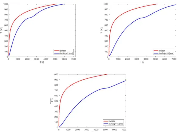
Figure 2 represents the temperature variation with time for the ISO-834 and unprotected steel plate, when the thickness of steel plate increases, in result the

temperature decreases.

Figure 2 : The temperature variation with time for ISO834 and unprotected steel plate.

(33)

(34)

Figure 4 : The temperature variation with time for ISO834 and protected steel plate, ds = 7.5.

Figure 5 : The temperature variation with time for ISO834 and protected steel plate, ds = 10.

(35)

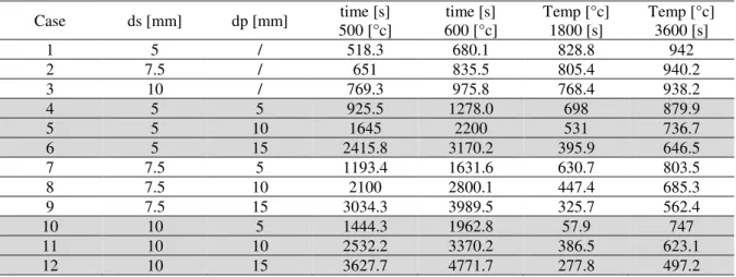
Table 2 - Results of protected and unprotected steel in Matlab.

Where ds is the thickness of the steel plate and dp is the thickness of the insulation Case ds [mm] dp [mm] time [s]

500 [°c]

time [s] 600 [°c]

Temp [°c] 1800 [s]

Temp [°c] 3600 [s]

1 5 / 518.3 680.1 828.8 942

2 7.5 / 651 835.5 805.4 940.2

3 10 / 769.3 975.8 768.4 938.2

4 5 5 925.5 1278.0 698 879.9

5 5 10 1645 2200 531 736.7

6 5 15 2415.8 3170.2 395.9 646.5

7 7.5 5 1193.4 1631.6 630.7 803.5

8 7.5 10 2100 2800.1 447.4 685.3

9 7.5 15 3034.3 3989.5 325.7 562.4

10 10 5 1444.3 1962.8 57.9 747

11 10 10 2532.2 3370.2 386.5 623.1

(36)

Chapter 4:

CONE CALORIMETER EXPERIMENTAL TESTS

The cone calorimeter is a fire testing device based on the principle of oxygen consumption during combustion, used to study the fire behaviour of small samples of various materials in condensed phase, and this device is used by the most leading fire research groups as a data source for properties of materials and as a source for inputting data to models when predicting fire behaviour. It gathers data regarding the ignition time, mass loss, combustion products, heat release rate and other parameters associated with its burning properties, (see Figure 6).

Figure 6: Picture of the Cone Calorimeter.

(37)

this application is performance of construction materials for construction and technical fire protection in according to EN standard in all the fields of building construction and industrial construction, [11].

In this chapter, we talk about the result of the experimental test and the steps for how to make the test, we use the cone calorimeter to measure the temperature according to specimen. For the specimen, we have different carbon steel plate where they have 3.6, 7.75 and 14 [mm] thickness, the first step is, we test unprotected carbon steel plate and the second step is we test the protected carbon steel plate with two different insulation named promatect-200 and promatect-H. They have different thickness of 15 and 20 [mm].

4.2 Preparation of the specimens

In this step, the specimens are prepared firstly, in total, the tests will be done on 3 carbon steel plates, with different thickness, with the dimensions of (100 × 100) [mm²]. To do this laboratory test four steps should be done, the first step should be the preparation of the carbon steel plates, then cleaning with using the grinder machine (Figure 7), the second step should be the welding of the two thermocouples in the top of the steel plate and another two in the bottom. Thirdly, put the plate in the ceramic blanket (see Figure 8) and the last step is the calibration of calorimeter.

(38)

a) The thermocouples. b) The thermocouples type K are welded in surface plate.

c) The ceramic blanket. d) The prepared specimen. Figure 8: The specimen of the unprotected carbon steel plate prepared.

4.3 Calibration of the cone calorimeter:

Before testing the specimens to give the required heat flux calibration is done according to the ISO 13927, [12]. This calibration is a process which consist to stabilize the heat flux using the temperature Figure 9. A heat flux meter is placed under the cone heater at the point corresponding to the centre of the specimen surface and the temperature controller

adjusted until the required test heat flux is achieved, the three heat flux values needed are 35, 50 and 75 [kW/m2_{] and in order, the three temperature values are 657, 749 and 867 [°C].}

(39)

The Figure 10 shows schematic drawing of apparatus, where (1) Inner shell, (2) Refractory-fibre packing, (3) Thermocouple, (4) Outer shell, (5) Heating element and (6) Steel plate.

Figure 10: Schematic drawing of apparatus, [12].

4.4 Experimental tests for unprotected steel:

After preparing the specimens and calibrating the cone calorimeter, we start testing the specimens Figure 11, firstly set the distance between the bottom of the cone calorimeter and top of the specimen equal 15 [mm], secondly, turn on the cone calorimeter and the computer, after that start increasing the temperature of the cone calorimeter to reach the required heat flux. The spacimen is covered by heat isolant. We put it under the cone calorimeter, run the software with this and remove the isolant at the same time.

Figure 11: Cone calorimeter and experimental setup.

(40)

and heat flux. With the passage of time when the heat flux increases the temperature also increase.

For example, having a 3.6 [mm] thickness plate, in Table 8 we see that the maximum temperature for minimum heat flux (q=35 [kw/m²]) is 600 [°C]; furthermore, the temperature increase upto 800 [°C] when the maximum heat flux is (q=75[kw/m²].

The same result comes from different thickness plate what is shown below on Table 9 and Table 10.

Figure 12: The temperature variation with time for the 3.6 [mm] thickness plate.

(41)

Figure 14: The temperature variation with time for the 14 [mm] thickness plate. From the graphs of above figures, the following table is obtained that shows the behavior of the steel plate under high temperature, as it can be seen in the Table 3, at same time the temperature decreases when we increase the thickness of the carbon steel plate. And also, when we increase the thickness of the steel plate, the time increases in a selected temperature.

And in another side, in heat flux q=35 [kw/m²], for 3.6 [mm] thickness of steel plate, it has 593 [°c] decreasing to 292.81 [°c] when the thickness plate is increasing to 14 [mm] at the same time 900[s]; more, it takes 375.5[s] for 3.6[mm] thickness plate where for 14 [mm] it increases to 2267.5[s]. The same output will come for heat flux q=50 and q=75 [kw/m²] as well as.

Table 3 - Results of experimental test of unprotected steel plate. q

[kw/m²] Ds [mm]

Taverage [°c] time[s]

900 [s] 1800 [s] 2700 [s] 3600 [s] 300 [°c] 400 [°c] 500

[°c] 600 [°c]

35

3.6 593 607.1 607.24 610.55 152.5 241.5 375.5 1044.5 7.75 528.99 585.68 591.16 594 315.5 494 769.5 /

14 292.81 439.85 536.36 564.43 935 1527 2267.5 /

50

3.6 702.52 705.26 704.60 705.41 111.5 165 231 325.5 7.75 619.99 656 660.38 662.58 209.5 318 470.5 770

14 496.03 620.61 645.61 654.13 405 623 913 1488

75

(42)

4.5 Experimental tests for protected steel:

In this step, it’s the same procedure for unprotected carbon steel plate; the difference is that we need to put the calcium silicate board in the upper side of the carbon steel plate in order to assure a protection, it has the same dimension with the carbon steel plate and two different calcium silicate board named PROMATECT-200 and PROMATECT-H, they have different thickness of 15 and 20 [mm], see

Figure 15.

a) Two calcium silicate plates of different thickness: 15 and 20 [mm].

b) Protected carbon steel plate with calcium silicate 15 [mm].

c) Protected carbon steel plate with calcium silicate plate 20[mm]

(43)

After preparing the specimen, we put it in the bottom of the cone calorimeter, where the distance is between the top of specimen and the bottom of the cone calorimeter is 25 [mm], see Figure 16.

Figure 16: Cone calorimeter and experimental setup.

4.6 Experimental tests for protected steel

About protected carbon steel plate with calcium silicate board which has 15 [mm] of thickness, by obtaining the following results transformed to graph in Figure 17, Figure 18 and Figure 19, it can be seen that the temperature of the steel plate increases slowly between 100 and 200 [°c] because the water starts to vaporize at 100 [° C]. After 200 [°c] we can see that there is a sharp increase in steel substrate temperature due to the total evaporation of water, [13].

(44)

Figure 18: The temperature variation with time for the 7.75 [mm] thickness plate and dp 15 [mm].

Figure 19: The temperature variation with time for the 14 [mm] thickness plate and dp 15[mm].

After getting result from above graphs, the following (Table 4) is obtained that shows the behavior of the steel plate under high temperature as the result for experimental test of protected steel with different thickness with the same insulation of 15 [mm] thickness and different heat flux in special temperature and special times.

(45)

So, finally on 400 [°c] for 4 [mm] thickness plate it takes 3347 [s] when the heat flux is q=35 [kw/m²]. On the mentioned temperature with heat flux it takes 2474 [s] when the heat flux is q=50 [kw/m²] and 1787 [s] when the heat flux is q=75 [kw/m²].

The steel is more protected when the thickness of steel is increased in the same heat flux and in another side we see that when the heat flux increases in the same thickness of steel plate, the steel takes short time for heating and in result it is less protected.

Table 4 - Results of experimental test of protected steel dp=15[mm]. q

[kw/m²] ds [mm]

900 [s] 1800 [s] 2700 [s] 3600 [s] 200 [°c] 300 [°c] 400 [°c]

500 [°c]

35

3.6 132.71 272.21 368.64 407.68 1407.5 1986 3347 / 7.75 106.03 189.74 276.30 326.74 1886.5 3057 / / 14 88.02 136.12 198.94 247.27 2717.5 / / /

50

3.6 140.48 323.33 415.97 452.53 1219 1664.5 2474 / 7.75 121.51 247.18 340.87 392.96 1490 2238.5 / / 14 92.86 163.79 235.83 290.13 2219.5 / / /

75

3.6 178.31 402.08 489.97 524.11 977.5 1299 1787 2896 7.75 148.67 332.48 435.06 486.36 1138 1607 / /

14 135.78 270.47 369.16 435.98 1313 2035.5 3072 /

Here, for Figure 20, Figure 21 and Figure 22 and Table 5 it is 20 [mm] of thickness steel plate and we get different value of result like the same conclusion done in previous experimental test using protected carbon steel plate with 15 [mm] thickness of calcium silicate board.

(46)

Figure 21: The temperature variation with time for the 7.75 [mm] thickness plate and dp 20 [mm].

Figure 22: The temperature variation with time for the 14 [mm] thickness plate and dp 20 [mm].

Table 5 - Results of experimental test of protected steel dp=20[mm]. q

[kw/m²] ds [mm]

900 [s] 1800 [s] 2700 [s] 3600 [s] 200 [°c] 300 [°c] 400 [°c] 500 [°c]

35

3.6 130.67 255.26 332.98 372.38 1357.5 2251 / / 7.75 109.06 206.78 275.69 321.26 1728.5 3128 / / 14 80.17 143.72 200.43 244.04 2691.5 / / /

50

3.6 171.13 329.99 413.38 448.30 1040.5 1593 2496 / 7.75 109.53 216.30 293.79 343.96 1643.5 2790.5 / / 14 99.31 188.81 260.15 312.62 1925 3356 / /

75

3.6 249.03 440.47 516.12 542.24 733 1086.5 1543 2415 7.75 190.73 349.89 442 492.92 943 1467.5 2222.5 /

(47)

4.7 Comparison between the unprotected and protected carbon steel plate

Now, it is needed to make the last result of unprotected and protected carbon steel plate in the same graph, see graph of Figure 23 and Figure 24, that shows us the temperature variation with time, different heat flux and different thickness steel plate. The temperature is higher in unprotected carbon steel plate than protected carbon steel plate.

For instance, in Figure 23(a) for q=35, q=50 and q=75 [kw/m²] heat flux, the maximum temperature for unprotected steel plate is 610.55, 705.41 and 805.05 [°c]; for protected steel is 407.68, 452.53 and 524.11 [°c].

So, the result comes for 3.6 [mm] thickness protected steel plate is that the temperature decreases between 64.15% and 66.77% than unprotected steel plate, for 7.75 [mm] thickness protected steel plate it is between 55.00% and 66.46% and finally for 14 [mm] it is between 43.81% and 55.39% than unprotected steel plate.

a) for 3.6 [mm] thikness plate b) for 7.75 [mm] thikness plate

c) for 14 [mm] thikness plate

(48)

Again, in Figure 24(a) for q=35, q=50 and q=75 [kw/m²] heat flux, it is the same thickness plate of Figure 23(a) what has the same maximum temperature for unprotected steel plate but now it is different insulation of 20 [mm] thickness. Moreover, about the maximum temperature for protected steel plate is 372.38, 448.30 and 542.24 [°c].

Here, for 3.6[mm] thickness protected steel plate the outcome we get is the temperature decreases between 60.99% and 67.35% than unprotected steel plate; for 7.75 [mm] it is between 51.91% and 67.35%; ultimately for 14 [mm] it is between 43.24% and 47.79% than unprotected steel plate.

In conclusion, from the above explanation and examples, the outcome comes for comparison between unprotected and protected steel plate that protected steel plate absorbs more temperature when the thickness of steel plate increases.

Figure 24 presents the comparison between protected and unprotected experimental test is the steel plate absorbs more energy when the thickness of steel plate increases.

a) for 3.6 [mm] thickness plate b) for 7.75 [mm] thickness plate

c) for 14 [mm] thickness plate

(49)

4.8 Measure the mass loss of calcium silicate board

An experimental test was made to know the mass loss of the insulation (calcium silicate board) and to measure the mass loss after 24h at 100 [°c], which is presented in Figure 25, we put the result in Table 6. Also, the thermal properties of the calcium silicate board were used in Table 9 and Table 10 and for the reaction of calcium silicate board in Table 8.

a) Mass before testing of thickness plate dp=20 [mm]

b) Mass after testing of thickness plate dp=20 [mm]

c) Mass before testing of thickness plate dp=15 [mm]

d) Mass after testing of thickness plate dp=15 [mm]

Figure 25 : Mass loss after 24 h at 100 [°c].

After measuring the mass loss of the calcium silicate board, results are presented in Table 6, where the mass loss of thickness dp = 15 [mm] is 15.9% moisture content, and 3%

(50)

Table 6 – Mass loss of calcium silicate board with different thickness. dp [mm] M0 [g] Mfinal [g] Mass loss % moisture

15 117.1508 98.4774 15.9%

(51)

Chapter 5:

THE HEAT TRANFER EQUATION BY THE FINITE

DIFFERENCE METHOD

The finite difference method is one of several techniques for obtaining numerical solutions to Eq (10). In all numerical solutions, the continuous partial differential equation (PDE) is replaced with a discrete approximation. In this context, the word “discrete” means that the numerical solution is known only at a finite number of points in the physical domain. The number of those points can be selected by the user of the numerical method. In general, increasing the number of points not only increases the resolution (i.e., detail), but also the accuracy of the numerical solution, [14].

The discrete approximation results in a set of algebraic equations that are evaluated (or solved) for the values of the discrete unknowns.

The mesh is the set of locations where the discrete solution is computed. These points are called nodes, and if one is to draw lines between adjacent nodes in the domain the resulting image would resemble a net or mesh. Two key parameters of the mesh are Δx, the local distance between adjacent points in space and Δt, the local distance between adjacent time steps. For the simple examples considered in this article Δx and Δt are uniform throughout the mesh, [14].

In the next sections, the development of a numerical method will be presented and a solution is obtained for unprotected steel plates and plates with fire insulation.

5.2 Steel and insulation energy equation

Making a program in Matlab in which the compare between experimental and numerical result can be done.

(52)

ρ𝑠𝑐𝑠𝜕𝑇_{𝜕𝑡 =}_{𝜕𝑥 (𝑘}𝜕 𝜕𝑇_{𝜕𝑥) + 𝑞}𝑔𝑒𝑛′′′ (10)

Also, Eq(10) works in initial boundary condition Eq(11) and boundary condition Eq(12) and Eq(13).

Figure 26 : Schematic drawing for specimen.

Initial boundary condition

boundary condition

In (14, x = ds is the thermal equilibiration (see Figure 26).

If t=0 𝑇(𝑥, 𝑡 = 0) = 𝑇₀ (11)

If

x=ds+dp 𝑘

𝜕𝑇

𝜕𝑥 = 𝑞1(𝑡) = 𝜀𝑞0 − ℎ(𝑇 − 𝑇𝑠) − 𝜀𝜎(𝑇4− 𝑇𝑠4) (12)

If x=0 𝑘𝜕𝑇

𝜕𝑥 = 𝑞2(𝑡) = 0 (13)

Tsteel = T ins 𝐾_𝑠𝜕𝑇𝑠

𝜕𝑥 = 𝐾𝑖𝑛𝑠 𝜕𝑇𝑖𝑛𝑠

(53)

On the other hand, for protected carbon steel plate, Eq 14 is used to solve 𝑞_𝑔𝑒𝑛′′′ and to

be calculated as a function of space and time according to the manufactured solution described, [15].

Where Eq(15) shows the Generation equation, which is defined as a function of the pyrolysis rate 𝑞_𝑔𝑒𝑛′′′ and the heat-of-pyrolysis H. Here, H is positive value for endothermic pyrolysis.

By using Eq(15), the following equation can be obtained which is presented as Eq (16). When dt≈0, Eq (17) can be obtained from Eq (16)

By replacing Eq (17) in Eq (11) we obtain Eq (24) whereas, Eq (19) is obtained from Eq (18).

If the phase transition takes place instantaneously at a fixed temperature, then a mathematical function is presented in Eq (19), [16].

Where U is a step function with value zero when T < Tf and otherwise

𝛿(T − 𝑇𝑓) is the direct delta function, whose value is infinity at the transition temperature

Tf, but zero at all other temperatures, presented in Eq(20)

𝑞𝑔𝑒𝑛′′′ = 𝐻𝑑𝜌_{𝑑𝑡 ,}𝑠 (15)

𝑑𝑡 ≈ 0 𝑑𝜌𝑠

𝑑𝑡 = 𝑑𝜌𝑠

𝑑𝑇 × 𝑑𝑇

𝑑𝑡 , (16)

ρ𝑐𝑝𝜕𝑇_{𝜕𝑡 − 𝐻}𝑑𝜌_{𝑑𝑇 ×}𝑠 𝑑𝑇_{𝑑𝑡 =}_{𝜕𝑥 (𝑘}𝜕 𝜕𝑇_{𝜕𝑥) ,} (17)

𝜕𝑇

𝜕𝑡 (ρ𝑐𝑝− 𝐻 𝑑𝜌𝑠

𝑑𝑇 ) = 𝜕 𝜕𝑥 (𝑘

𝜕𝑇

𝜕𝑥) , (18)

(54)

To alleviate this singularity the direct delta function can be approximated by the normal distribution function in which is presented in Eq (21)

where ∆𝑇 is one-half of the assumed phase change interval.

The similar specific heat is gained by affixing to the basis standard additional energy which is necessary because of volatilization of water or endothermic reaction or by deducting from base value energy released in time of endothermic reaction. Here, the base value normally depends on temperature but the extent is usually small. Hence, a certain value may be used if the appropriate variation is not available.

For this study, specific heat of the insulation (calcium silicate board) has four reactions. Each reaction has two equations or each reaction is determined by two equations (see Table 8).

When a fire protection material increases in temperature, external energy is required. The required external energy is reduced if the fire protection material generates heat through exothermic reaction or increased if the fire protection material undergoes endothermic reaction or if water is evaporated. The amount of energy required to raise the temperature of unit mass material by 1 [°C] is defined as the specific heat of the material. In simplistic heat transfer analysis, an equivalent specific heat may be used to represent the combined effects. The equivalent specific heat is obtained by adding to the base value additional energy that is required due to endothermic reaction or evaporation of water or by deducting from the base value energy that is released during exothermic reaction. The base value is usually temperature dependent. However, the range of this change is usually small. Therefore, if the precise variation is not available, a constant value may be used. To allow for heat generated/consumed during exothermic/endothermic chemical reactions and heat consumed

𝑑∅

𝑑𝑇 = 𝛿(T − 𝑇𝑓) (20)

𝑑∅

𝑑𝑇 = 𝜖𝜋−1/2𝑒−𝜖

2_(T−𝑇

𝑓)2 , 𝜖 = 1

√2∆𝑇 (21)

𝜌𝑓 = 𝜌0− ∆𝜌[0.5 + 0.5 tanh (𝑇 − 𝑇_∆𝑇 𝑓

(55)

during water evaporation, a simple method is to distribute the energy involved through the temperature duration of the chemical reactions/water evaporation. The precise distribution may be difficult to quantify, but since the degree of accuracy required is not high, a triangular distribution may be conveniently used, [17], as represented in Figure 27.

Figure 27: Triangular variation of specific heat during moisture evaporation. The effect of moisture evaporation and other chemical reactions, on specific heat is simulated by assuming a simple mechanism driven only by the moisture concentration. It is assumed to take place during a temperature interval (with a specific heat given by:

The reaction starts at 𝑇_{𝑖𝑛𝑖𝑡𝑖𝑎𝑙} is the primary temperature, 𝑇_{𝑚𝑒𝑑𝑖𝑢𝑚} is the temperature in peak water evaporation and 𝑇_𝑒𝑛𝑑 is the final temperature; 𝑇₂ is the temperature for insulation, 𝐶𝑝₀ is the initial specific heat, 𝐶𝑝_𝑣 is moisture specific heat.

Where H is enthalpy for each reaction and moisture percentage is dependent on Table 8. More, T is interval of each reaction, T2 is temperature of insulation.

𝐶𝑝= Cp0+ Cp𝑣 (23)

(56)

5.3 The finite difference method

Applying the finite-difference method to a differential equation involves replacing all derivatives with difference formulas. In the heat equation, there are derivatives with respect to time and derivatives with respect to space. Using different combinations of mesh points

in the difference formulas results in different schemes. In the limit as the mesh spacing (Δx and Δt) go to zero, the numerical solution obtained with any useful1 scheme will approach the true solution to the original differential equation.

Figure 28: Finite Difference discretization of a function u or T. Consider a Taylor series expansion u(x) about the point xi



  

.... ! 3 2 3 3 3 2 2 2                 i i

i x x

x i i x u x x u x x u x x u x x u ₍₂₅₎

Solve for (∂u/∂x)xi

 



  

.... ! 3 2 3 3 2 2                  i i

i x x

i i x i x x u x x u x x x u x x u x u x u ₍₂₆₎

Substitute the approximate solution for the exact solution.

i

i-1

i+1



x=h



x=h

u

i-1

u

i

u

i+1

i-2

i+2

(57)

 

x O x

u u

u i i

x _  



 1 ₍₂₇₎

This equation is called the forward difference formula for (∂u/∂x)xi because it involves

nodes xi and xi+1. The forward difference approximation has a truncation error that is O(Δx). The size of the truncation error is (mostly) under our control because we can choose the mesh size Δx.

Finite difference approximations to higher order derivatives can be obtained with the additional manipulations of the Taylor Series expansion about u(xi).

.... ! 4 2 2 ₄ 4 4 2 2 2 1

1 _ 

         _  i i x x i i i x u x x u x u u

u , ₍₂₈₎

This is also called the central difference approximation, but it is the approximation to the second derivative.

 

2 2

1

1 2 _O _x

x u u u

u i i i

xx _  

 

  

(29)

5.4 Method of Lines

The author A. Vande Wouwer et al in 2001 discussed a system of PDEs with u which is a dependent vector. A vector is denoted by a bold face and a partial deriavative is denoted by a subscript. About the coordinates, Cartesian, Cylinderical and Spherical have components of (x, y, z), (r, θ, z) and (r, θ, φ), [18].

A general equation considering PDE problem is described where the equation encloses in one, two and three spatial dimensions plus time, Eq (30)

ut = f (u),

XL < X < XR, t > 0

(58)

Here, ut = 𝜕𝑢

𝜕𝑡 is the first order partial deriavative of u with respect to t, u is vector of

dependent variables, t is initial value independent variable, x is boundary value independent variables, f is spatial differential operator f (x, t, u, ux, uxx….), [18].

For instance, the scalar advection Eq (31) comes from the spatial differential operator f if f (x, t, u, ux, uxx….) = −𝑣𝑢_𝑥

Where ux = 𝜕𝑢

𝜕𝑥is the first order partial deriavative of u with respect to x, 𝑣 is the

velocity as constant.

PDE problems like Eq (30) is solved by the Method of Lines (MOL) which is a computational approach and that emanates into two different steps. Firstly, the spatial deriavatives and secondly, the resulting system of semi-discrete ODEs in the initial value variable is integrated in time, t.

According to the mentioned book, representing the MOL in Eq (31) gives us the Eq (33) using 2nd order centered FD in spatial deriavative at grid point i,

Then, substituting this estimation in Eq (31) with 𝑣 = 1 gives a system of N ODEs Eq (33)

Library ODE integrator can integrate the spatial grid index i what has the value similar to a system of N initial value of ODEs. Using the initial condition Eq (34) in boundary condition (i = 1 and i = N) gives us the fictitious point what is outside of the spatial domain, [18]. The integrator used in this work was the ode15s from the Matlab library.

𝜕𝑢 𝜕𝑡 = −𝑣

𝜕𝑢

𝜕𝑥 (31)

𝜕𝑢 𝜕𝑥 = −𝑣

𝑢𝑖 − 𝑢𝑖−1

2∆𝑥 + 𝑂(∆𝑥2), 𝑖 = 1, 2, … , 𝑁 (32)

𝑑𝑢𝑖 𝑑𝑡 = −

𝑢𝑖+1− 𝑢𝑖−1

(59)

About Spatial Discretization, to show the concept of upwinding in the book it is used as the approximation of 𝜕𝑢

𝜕𝑥 in Eq (31) the first order, two-point upwind FD, Eq (35)

In Eq (36) the system of ODEs comes

In Eq (35) the approximation for 𝜕𝑢

𝜕𝑥 is called an upwind FD as it uses, besides to

the point of the approximation, i, the point upwind, i -1 (for 𝑣 > 0), but not the point downwind i+1.

More about time integration, a system of ODEs with widely separated eigenvalues called stiff ODEs is produced by spatial discretization. ∆𝑥 – which is usually equal to the order of the highest spatial deriavative the time step restriction in a finely gridded region with small ∆𝑥 that can be more acute than in coarsely gridded region as the durability limitation of an obvious time integration method is inversely proportional to some power of the grid spacing. A wide choice option of quality library ODE is available, even, one of the big benefits of the MOL approach to PDE systems is the scope to use the progression in ODE integrators and their associated codes, [18].

5.5 Comparison between experimental and numerical results of unprotected

steel

When the program was prepared, for unprotected carbon steel plate the experimental results were used and obtained the following results transformed to graph charts and for the program see (ANNEX A3).

𝑢(𝑥, 0) = 𝑓(𝑥) (34)

𝜕𝑢 𝜕𝑥 =

𝑢𝑖− 𝑢𝑖−1

∆𝑥 + 𝑂(∆𝑥), 𝑖 = 1, 2, … , 𝑁 (35)

𝑑𝑢𝑖 𝑑𝑡 = −𝑣

𝑢𝑖 − 𝑢 𝑖 − 1

(60)

From Figure 29 to Figure 37, a variation of temperature is noticed through out the time and shows the numerical and experimental results with different thikness and different heat flux in which all results are similar. Whereas, a change in temperature is noticed in the curve of the numerical results what is presented in the Figure 31, Figure 34 and Figure 37 above 700[°C]. These changes are due to the presence of the peak of the specific heat of steel in 700[°C] that is presented in Figure 1.

Figure 29: Results of the numerical method and experimental with thickness ds=3.6[mm] and heat flux q=35[KW/m²].

(61)

Figure 31: Results of the numerical method and experimental with thickness ds=3.6[mm] and heat flux q=75[KW/m²].

Figure 32: Results of the numerical method and experimental with thickness ds=7.75[mm] and heat flux q=35 [KW/m²].

(62)

Figure 34: Results of the numerical method and experimental with thickness ds=7.75[mm] and heat flux q=75[kw/m²].

Figure 35: Results of the numerical method and experimental with thickness ds=14[mm] and heat flux q=35[kw/m²].

(63)

Figure 37: Results of the numerical method and experimental with thickness ds=14[mm] and heat flux q=75[kw/m²].

All results from the graphs were converted into values which were presented in Table 7. Analysis of results, showed variation of temperature through out time, thickness of steel plate and heat flux in which the temperature from carbon steel plate was very similar in the experimental and numerical result.

For the heat flux 35 q [kw/m²], the error for the experimental and numerical result is very similar dependent between 1.32% and 2.78% in 3.6 [mm] thickness steel plate. Moreover, in 7.75 [mm] thickness steel plate the error for both result is between 0.14% and 6.07%; in 14 [mm] it is dependent between 1.75% and 11.69%. The same thing happens for heat flux 50 and 75 q [kw/m²].

Table 7 – The result of temperature between experimental and numerical result for unprotected steel plate.

q[kw/m²] ds[mm] Temperature [°c]

900 [s] 1800 [s] 2700 [s] 3600 [s] T-top[°c] TBot[°c] T-top[°c] TBot[°c] T-top[°c] TBot[°c] T-top[°c] TBot[°c]

35

3.6 Ex 593 593 607 606 607 607 611 611

Nu 585 585 594 594 594 594 594 594

7.75 Ex 528 528 587 586 592 591 594 593

Nu 497 496 582 582 593 593 593 593

14 Ex 406 403 524 524 549 548 555 553

Nu 359 356 514 513 569 568 569 568

50

3.6 Ex 702 702 705 705 704 704 704 704

Nu 674 674 679 679 679 279 679 679

7.75 Ex 620 619 656 656 660 660 662 661

Nu 606 606 672 672 678 678 679 679

14 Ex 542 537 639 638 654 653 657 656

Nu 470 466 623 622 664 644 675 674

75

3.6 Ex 798 798 802 802 804 803 804 804

Nu 779 778 784 784 784 784 784 784

7.75 Ex 751 748 787 786 791 790 792 791

Nu 726 725 775 775 784 784 784 784

14 Ex 663 655 753 750 780 779 785 784

(64)

5.1 Comparison between experimental and numerical result of protected

steel

Table 8 represents the reaction of calcium silicate board where it absorbs 2330 [kj/kg] in a specific temperature [75°C] interval between 25 and 100 [°C] for evaporation of free water in first reaction and in second reaction it absorbs 1440 [kj/kg] in a specific temperature 125 [°C] interval between 100 and 400 [°C] for dehydration of calcium silicate board, Moreover, calcium silicate board absorbs 450 [kj/kg] in specific temperature 450 [°C] in interval between 400 and 600 [°C] for dehydration of calcium hydroxide , Finally the last reaction absorbs 750 [kj/kg] in a specific temperature 750°C between 600 and 1000 [°C] for decarbonation, [13].

Table 8 - Thermal Conductivity and Heat Capacity of Mild Steel vs. Temperature, [13].

∆𝑇[°c] Treaction [°c] Mass loss [kg] Enthalpy [kj/kg] ∆𝑚total[kg] Evaporation of free

water 25 to 100

75 9% 2330

12% Dehydration of

‘calcium silicate hydrate get’

100 to 400

125 23.5% 1440

Dehydration of calcium hydroxide

400 to 600

450 21.5% 450

decarbonation

600 to 1000 750 46% 750

(65)

Table 9 – Thermal properties of Promatect-200, [10].

T [°c] λ [w/mk] ρ [kg/m3_]

20 0.189 835

Table 10 - Thermal properties of Promatect-H, [19].

T[°C] λw/mk Cp(400 °C)KJ/KgK ρKg/m³ moisture

20 0.17

0.92 870 5,95%

100 0.19

200 0.21

After making the program for the reaction of the calcium silicate board, it can be seen that the result in Figure 38 shows the parametric analysis of the moisture evaporation and for the Figure 38(a) we can see (1) is the first reaction (dT1= 5 [°c]), (2) is the second reaction (dT2= 150 [°c]), (3) is the third reaction (dT3= 100 [°c]) and (4) is the last reaction (dT4=200 [°c]). Finally, for Figure 38(b) and (c) the same interval for all reactions but changing the first reaction dT1 = 25 [°c] for (b) and 50 [°c] for (b).

a) Interval for the first reaction dT1=5 [°c]

b) Interval for the first reaction dT1=25 [°c]

(66)

Figure 39 : Specific mass variation with temperature.

Now, after preparing the program, for protected carbon steel plate the experimental results are used and get the following results what are transformed to graph charts and for the program, it is the same of (ANNEX A3) but the difference for the function of ‘Solve

Parabolic’, see (ANNEX A4).

According to curves presented in Figure 40, Figure 41 and Figure 42, evaporation of water occurred in range of temperature from 25 to 100[°C]. Above 100[°C], curves of the experiemental and numerical results increase normally through out time.

a)Temperature variation with time in heat flux q= 35 [kw/m²]

(67)

c)Temperature variation with time in heat flux q= 75 [kw/m²]

Figure 40: The experimental result and numerical result of protected carbon steel plate ds=3.6 [mm] with insulation dp=15 [mm] thickness.

b)Temperature variation with time in heat flux q= 50 [kw/m²]

c)Temperature variation with time in heat flux q= 75 [kw/m²]

(68)

b) Temperature variation with time in heat flux q= 50 [kw/m²]

c) Temperature variation with time in heat flux q= 75 [kw/m²]

Figure 42: The experimental result and numerical result of protected carbon steel plate ds=14 [mm] with insulation dp=15 [mm] thickness.

As it was done in protected carbon steel plate, all curves were represented into values in the following table that shows the behavior of the steel plate under high temperature

(69)

Table 11, also shows the results of experimental and numerical tests of protected steel plate with different thickness with the same insulation of 15 [mm] and different heat flux during 15, 30, 45 and 60 [min].

For the heat flux 35 q [kw/m²], the error for the experimental and numerical result is similar dependent between 0.75% and 10.48% in 3.6 [mm] thickness steel plate. Moreover, in 7.75 [mm] thickness steel plate the error for both result is between 24.48% and 29.72%; in 14 [mm] it is dependent between 0.51% and 27.51%. Here, the same thing also happens for heat flux 50 and 75 q [kw/m²].

Table 11 - The result of temperature between experimental and numerical result for protected steel plate with dp =15 [mm].

q[kw/m²] ds[mm] 900[°c] 1800[°c] 2700[°c] 3600[°c] T-top[°c] TBot[°c] T-top[°c] TBot[°c] T-top[°c] TBot[°c] T-top[°c] TBot[°c]

35

3.6 Ex 133 132 272 271 369 367 407 405

Nu 133 133 284 284 400 400 453 453

7.75 Ex 98 97 163 161 243 241 294 292

Nu 139 139 251 250 331 331 389 389

14 Ex 88 87 136 135 199 198 245 245

Nu 64 63 137 136 201 201 255 255

50

3.6 Ex 141 139 324 322 416 415 452 450

Nu 174 174 351 350 442 448 485 485