www.geosci-model-dev.net/9/697/2016/ doi:10.5194/gmd-9-697-2016
© Author(s) 2016. CC Attribution 3.0 License.
ASHEE-1.0: a compressible, equilibrium–Eulerian model for
volcanic ash plumes
M. Cerminara1,2,3, T. Esposti Ongaro2, and L. C. Berselli3 1Scuola Normale Superiore, Pisa, Italy
2Istituto Nazionale di Geofisica e Vulcanologia, Sezione di Pisa, Pisa, Italy 3Dipartimento di Matematica, Università degli Studi di Pisa, Pisa, Italy
Correspondence to:M. Cerminara ([email protected])
Received: 4 September 2015 – Published in Geosci. Model Dev. Discuss.: 19 October 2015 Revised: 20 January 2016 – Accepted: 20 January 2016 – Published: 18 February 2016
Abstract. A new fluid-dynamic model is developed to nu-merically simulate the non-equilibrium dynamics of polydis-perse gas–particle mixtures forming volcanic plumes. Start-ing from the three-dimensional N-phase Eulerian transport equations for a mixture of gases and solid dispersed particles, we adopt an asymptotic expansion strategy to derive a com-pressible version of the first-order non-equilibrium model, valid for low-concentration regimes (particle volume frac-tion less than 10−3) and particle Stokes number (St– i.e., the ratio between relaxation time and flow characteristic time) not exceeding about 0.2. The new model, which is called ASHEE (ASH Equilibrium Eulerian), is significantly faster than the N-phase Eulerian model while retaining the capa-bility to describe gas–particle non-equilibrium effects. Direct Numerical Simulation accurately reproduces the dynamics of isotropic, compressible turbulence in subsonic regimes. For gas–particle mixtures, it describes the main features of den-sity fluctuations and the preferential concentration and clus-tering of particles by turbulence, thus verifying the model re-liability and suitability for the numerical simulation of high-Reynolds number and high-temperature regimes in the pres-ence of a dispersed phase. On the other hand, Large-Eddy Numerical Simulations of forced plumes are able to repro-duce the averaged and instantaneous flow properties. In par-ticular, the self-similar Gaussian radial profile and the de-velopment of large-scale coherent structures are reproduced, including the rate of turbulent mixing and entrainment of atmospheric air. Application to the Large-Eddy Simulation of the injection of the eruptive mixture in a stratified at-mosphere describes some of the important features of tur-bulent volcanic plumes, including air entrainment, buoyancy
reversal and maximum plume height. For very fine particles (St→0, when non-equilibrium effects are negligible) the model reduces to the so-called dusty-gas model. However, coarse particles partially decouple from the gas phase within eddies (thus modifying the turbulent structure) and prefer-entially concentrate at the eddy periphery, eventually being lost from the plume margins due to the concurrent effect of gravity. By these mechanisms, gas–particle non-equilibrium processes are able to influence the large-scale behavior of volcanic plumes.
1 Introduction
After injection in the atmosphere, this multiphase erup-tive mixture can rise convecerup-tively in the atmosphere, either forming a buoyant volcanic plume or collapsing catastroph-ically forming pyroclastic density currents. These two end-members have different spatial and temporal scales and dif-ferent impacts on the surrounding of a volcano. Understand-ing the dynamics of volcanic columns is one of the topical aims of volcanology and the main motivation for this work.
The term volcanic column will be adopted in this pa-per to generically indicate the eruptive character (e.g., con-vective/collapsing column). Following the fluid-dynamic nomenclature, we will term jet the inertial regime of the
volcanic column and plume the buoyancy-driven regime.
A forced plume is characterized by an initial momentum-driven jet stage, transitioning into a plume.
In this work, we present a new computational fluid-dynamic model to simulate turbulent gas–particle forced plumes in the atmosphere. Although the focus of the paper is on subsonic regimes, the model is also suited to be applied to transonic and supersonic flows. In many cases, indeed, the eruptive mixture is injected into the atmosphere at pressure higher than atmospheric, so that the flow is initially driven by a rapid, transonic decompression stage. This is suggested by numerical models predicting choked flow conditions at the volcanic vent (Wilson, 1980; Wilson et al., 1980), im-plying a supersonic transition above the vent or in the crater (Kieffer, 1984; Woods and Bower, 1995; Koyaguchi et al., 2010) and it is supported by field evidences of the emission of shock waves during the initial stages of an eruptions (Mor-rissey, 1997). Despite the importance of the decompression stage for the subsequent development of the volcanic plume (Pelanti and LeVeque, 2006; Ogden et al., 2008b; Orescanin et al., 2010; Carcano et al., 2013) and for the stability of the eruptive column (Ogden et al., 2008a), our analysis is lim-ited to the plume region where flow pressure is equilibrated to the atmospheric pressure. From laboratory experiments, this is expected to occur within less than 20 inlet diameters above the ground (Yüceil and Ötügen, 2002).
A wide set of numerical tests are presented in this paper (Sect. 4) to assess the adequacy of the model for the intended volcanological application (Sect. 5) and the reliability of the numerical solution method.
1.1 Dusty-gas modeling of volcanic plumes
Starting from the assumption that the large-scale behavior of volcanic columns is controlled by the bulk properties of the eruptive mixture, most of the previous models of vol-canic plumes have considered the eruptive mixture as homo-geneous (i.e., they assume that particles are perfectly coupled to the gas phase). Under such a hypothesis, the multiphase transport equations can be largely simplified and reduce to a set of mass, momentum and energy balance equations for a single fluid (named dusty-gasor pseudo-gas) having av-erage thermo-fluid dynamic properties (mixture density,
ve-locity and temperature) and an equation of state accounting for the incompressibility of the particulate phase and gas co-volume (Marble, 1970).
By adopting the dusty-gas approximation, volcanic plumes have been studied in the framework of jet (Prandtl, 1963) and plume theory (Morton et al., 1956; Morton, 1959). One-dimensional, steady-state dusty-gas models of volcanic plumes have thus had a formidable role in volcanology to identify the main processes controlling their dynamics and scaling properties (Wilson, 1976; Woods, 1988; Sparks et al., 1997).
Accordingly, volcanic plume dynamics are schematically subdivided into two main stages. The lower, jet phase is driven by the initial flow momentum. Mixture buoyancy is initially negative (the bulk density is larger than atmospheric) but the mixture progressively expands adiabatically thanks to atmospheric air entrainment and heating, eventually under-going a buoyancy reversal. When buoyancy reversal does not occur, partial or total collapse of the jet from its maximum thrust height and generation of pyroclastic density currents are expected.
Above the jet thrust region, the rise of volcanic plumes is driven by buoyancy and it is controlled by turbulent mixing until, in the stratified atmosphere, a level of neutral buoyancy is reached. Above that level, the plume rises up to its maxi-mum height and then starts to spread out as a gravity current (e.g., Costa et al., 2013) forming an umbrella ash cloud dis-persing in the atmosphere and slowly falling-out.
In one-dimensional, time-averaged models, entrainment of atmospheric air is described by one empirical coefficient (the entrainment coefficient) relating the influx of atmospheric air to the local, vertical plume velocity. The entrainment coeffi-cient also determines the plume shape (Ishimine, 2006) and can be empirically assessed by means of direct field observa-tions or ad hoc laboratory measurements.
Further development of volcanic plume models have in-cluded the influence of atmospheric stratification and humid-ity (Woods, 1993; Glaze and Baloga, 1996), the effect of crosswind (Bursik, 2001), loss and re-entrainment of solid particles from plume margins (Woods and Bursik, 1991; Veitch and Woods, 2002), wet aggregation (Folch et al., 2015) and transient effects (Scase, 2009; Woodhouse et al., 2015). However, one-dimensional models strongly rely on the self-similarity hypothesis, whose validity cannot be ex-perimentally ascertained for volcanic eruptions.
To overcome the limitations of one-dimensional models, three-dimensional dusty-gas models have been developed to simulate volcanic plumes. Suzuki (2005) have developed a three-dimensional dusty-gas model (SK-3D) able to ac-curately resolve the relevant turbulent scales of a volcanic plume, allowing a first, theoretical determination of the en-trainment coefficient (Suzuki and Koyaguchi, 2010), without the need of an empirical calibration.
microphysics of water in volcanic plumes, the ATHAM (Ac-tive Tracer High Resolution Atmospheric Model) code has been designed (Oberhuber et al., 1998; Graf et al., 1999; Van Eaton et al., 2015). ATHAM describes the dynamics of gas– particle mixtures by assuming that particles are in kinetic equilibrium with the gas phase only in the horizontal compo-nent, whereas along the vertical direction they are allowed to have a differential velocity. Thermal equilibrium is assumed. In this sense, ATHAM relaxes the dusty-gas approximation (while maintaining its fundamental structure and the same momentum transport equations) by describing the settling of particles with respect to the gas.
1.2 Multiphase flow models of volcanic plumes
Notwithstanding all the above advantages, dusty-gas models are still limited by the equilibrium assumption, which can be questionable at least for the coarsest part of the granulometric spectrum in a plume. Turbulence is indeed a nonlinear, mul-tiscale process and the time and space scales of gas–particle interaction may be comparable with some relevant turbulent scales, thus influencing the large-scale behavior of volcanic plumes.
To model non-equilibrium processes, Eulerian multiphase flow models have been developed, which solve the full set of mass, momentum and energy transport equations for a mix-ture of gas and dispersed particles, treated as interpene-trating fluids. Valentine and Wohletz (1989), Dobran et al. (1993) and Neri and Dobran (1994) first analyzed the in-fluence of erupting parameters on the column behavior. By means of two-dimensional numerical simulations, they in-dividuated a region of transition from collapsing to convec-tive columns. Lately, two-dimensional (Di Muro et al., 2004; Dartevelle et al., 2004) and three-dimensional numerical sim-ulations (Esposti Ongaro et al., 2008) have contributed to further modify the view of a sharp transition between con-vecting and collapsing columns in favor of that of a tran-sitional regime, characterized by a progressively increasing fraction of mass collapsing. However, previous works could not investigate in detail the non-equilibrium effects in vol-canic plumes, mainly because of their averaged description of turbulence: a detailed resolution of the relevant turbulent scales in three dimensions would indeed be computationally prohibitive for N-phase systems.
The main objective of the present work is therefore to de-velop a new physical model and a fast three-dimensional nu-merical code able to resolve the spatial and temporal scales of the interaction between gas and particles in turbulent regimes and to describe the kinetic non-equilibrium dynamics and their influence on theobservablefeatures of volcanic plumes. To this aim, a development of the so-called equilibrium– Eulerian approach (Ferry and Balachandar, 2001; Balachan-dar and Eaton, 2010) has been adopted. It is a general-ization of the dusty-gas model keeping the kinematic non-equilibrium as a first-order correction of the Marble (1970)
model with respect to the Stokes number of the solid particles in the mixture. Here, we generalize the Ferry and Balachan-dar (2001) model to the compressible two-way case.
The derivation of the fluid dynamic model describing the non-equilibrium gas–particle mixture is described in detail in Sect. 2. The computational solution procedure and the nu-merical code development are reported in Sect. 3. Section 4 focuses on verification and evaluation issues in the context of applications to turbulent volcanic plumes. In particular, we discuss three-dimensional numerical simulations of com-pressible isotropic turbulence (with and without particles), experimental-scale forced plumes and the Sod (1978) shock tube problem. Finally, Sect. 5 presents numerical simulations of volcanic plumes and discusses some aspects related to nu-merical grid resolution in practical cases.
2 The multiphase flow model
To derive an appropriate multiphase flow model to de-scribe gas–particle volcanic plumes, we introduce the non-dimensional scaling parameters characterizing gas–particle and particle–particle interactions.
The drag force between gas and particles introduces into the system a timescaleτs, theparticle relaxation time, which is the time a particle needs to equilibrate to a change of gas velocity. Gas–particle drag is a nonlinear function of the local flow variables and, in particular, it depends strongly on the relative Reynolds number, defined as
Res= ˆ
ρg|us−ug|ds
µ . (1)
Here ds is the particle diameter, ρˆg is the gas density, µ is the gas dynamic viscosity and ug(s) is the gas (solid)
phase velocity field. With ρˆg(s) being the gaseous (solid)
phase density and ǫs=Vs/V the volumetric concentration of the solid phase, it is useful to define the gas bulk den-sityρg≡(1−ǫs)ρˆg≃ ˆρgand the solid bulk densityρs≡ǫsρˆs (even though in our applicationsǫsis order 10−3,ρs is non-negligible sinceρˆs/ρˆgis of order 103).
For an individual point-like particle (i.e., having diameter ds much smaller than the scale of the problem under analy-sis), atRes<1000, the drag force per volume unity can be given by Stokes’ law:
fs=ρs τs
(ug−us), (2)
where τs≡ρˆs
ˆ
ρg ds2
18ν φc(Res) (3)
et al., 1978; Balachandar, 2009; Balachandar and Eaton, 2010; Cerminara, 2016) and for spherical particles (Ganser, 1993). In Eq. (2) we disregard all effects due to the pres-sure gradient, the added mass, the Basset history and the Saffman terms, because we are consideringheavy particles:
ˆ
ρs/ρˆg≫1 (see Ferry and Balachandar, 2001; Bagheri et al., 2013). Equation (2) has a linear dependence on the fluid– particle relative velocity only whenRes≪1, so thatφc≃1 and the classic Stokes drag expression is recovered. On the other hand, if the relative Reynolds numberRes grows, non-linear effects become much more important in Eq. (3). The Clift et al. (1978) empirical relationship used in this work has been used and tested in a number of papers (e.g., Wang and Maxey, 1993; Bonadonna et al., 2002; Balachandar and Eaton, 2010), and it is equivalent to assuming the following gas–particle drag coefficient:
CD(Res)= 24
Res(1+0.15Re 0.687
s ). (4)
Wang and Maxey (1993) discussed nonlinear effects due to this correction on the dynamics of point-like particles falling under gravity in a homogeneous and isotropic turbulent sur-rounding. We recall here the terminal velocity that can be found by settingug=0 in Eq. (2) is
ws= s
4dsρˆs 3CDρgg
g=τsg. (5)
As previously pointed out, the correction used in Eq. (4) is valid ifRes<103, the regime addressed in this work for ash particles much denser then the surrounding fluid and smaller than about 1 mm. As shown by Balachandar (2009), maxi-mum values ofResare associated with particle gravitational settling (not with turbulence). Using Eqs. (4) and (5), it is thus possible to estimate theResof a falling particle with di-ameterds. We obtain thatResis always smaller than 103for ash particles finer than 1 mm in air. If regimes with a stronger decoupling need to be explored, more complex empirical cor-rections have to be used forφc(Neri et al., 2003; Bürger and Wendland, 2001). It is also worth noting that ash particles can differ significantly from spheres and terminal settling veloc-ities of volcanic particles can be up to a factor 2–3 with re-spect to spherical assumption. To account for this effect vari-ous modifications to Eq. (4) have been devised (e.g., Dellino et al., 2005; Pfeiffer et al., 2005).
The same reasoning can be applied to estimate the ther-mal relaxation time between gas and particles. In terms of the solid phase specific heat capacityCsand its thermal con-ductivitykg, we have
τT =
2
Nus
ˆ
ρsCs kg
ds2
12, (6)
where Nus=Nus(Res,Pr) is the Nusselt number, usually function of the relative Reynolds number and of the Prandtl
number of the carrier fluid (Neri et al., 2003). In terms ofτT,
the heat exchange between a particle at temperatureTs and the surrounding gas at temperatureTgper unit volume is Qs=ρsCs
τT
(Ts−Tg). (7)
Comparing the kinetic and thermal relaxation times we get τT
τs = 3 2
2φc
Nus Csµ
kg . (8)
In order to estimate this number, firstly we notice that factor 2φc/Nus tends to 1 ifRes→0, and it remains smaller than
≃2 ifRes<103(Neri et al., 2003; Cerminara, 2016). Then, in the case of ash particles in air, we have (in SI units)µ≃ 10−5, C
s≃103,kg≃10−2. Thus we have that τT/τs≃1, meaning that the thermal equilibrium time is typically of the same order of magnitude as the kinematic one. This bound is very useful when we write the equilibrium–Eulerian and the dusty-gas models, because it ensures that the thermal Stokes number is of the same order as the kinematic one, at least for volcanic ash finer than about 1 mm.
The non-dimensional Stokes number (St) is defined as
the ratio between the kinetic relaxation time and a char-acteristic time of the flow under investigation τL, namely Sts=τs/ τL. The definition of the flow timescale can be
problematic for high-Reynolds number flows (typical of vol-canic plumes), which are characterized by a wide range of interacting length- and timescales, a distinctive feature of the turbulent regime. For volcanic plumes, the more energetic timescale would be of the order ofτL=L / U, whereLand
U are the plume diameter and velocity at the vent, which gives the characteristic turnover time of the largest eddies in a turbulent plume (e.g., Zhou et al., 2001). On the other hand, the smallest timescale (largestSts) can be defined by the Kolmogorov similarity law byτη∼τLRe−L1/2, where the
macroscopic Reynolds number is defined, at first instance, byReL=U L/ν, withνbeing the kinematic viscosity of the
gas phase numerical models. It is also useful to introduce the Large-Eddy Simulation (LES) timescale τξ, relative to the
LES length scaleξ. This is related to the numerical grid res-olution, size of the explicit filter and discretization accuracy (Lesieur et al., 2005; Garnier et al., 2009; Balachandar and Eaton, 2010; Cerminara et al., 2015). At LES scaleξ,Stsis not as large as at the Kolmogorov scale, thus the decoupling between particles and the carrier fluid is mitigated by the LES filtering operation. Dimensional analysis shows (see Sect. 5) thatSts.0.2 for LES of volcanic ash finer than about 1 mm.
The model presented here is conceived for resolving di-lutesuspensions, namely mixtures of gases and particles with volumetric concentration Vs
V ≡ǫs.10−
collisions. In the dilute regime, in which we can assume an equilibrium Maxwell distribution of particle velocities, the mean free path of solid particles is given by (Gidaspow, 1994)
λp-p= 1 6√2
ds
ǫs. (9)
Consequently, particle–particle collisions are relatively in-frequent (λp-p∼0.1 m≫ds), so that we can neglect, as a first approximation, particle–particle collisions and con-sider the particulate fluid as pressure-less, inviscid and non-conductive.
In volcanic plumes the particle volumetric concentra-tion can exceed by one order of magnitude the threshold ǫs≃10−3only near the vent (see, e.g., Sparks et al., 1997; Esposti Ongaro et al., 2008). However, the region of the plume where the dilute suspension requirement is not ful-filled remains small with respect the size of the entire plume, weakly influencing its global dynamics. Indeed, as we will show in Sect. 5, air entrainment and particle fallout induce a rapid decrease of the volumetric concentration. In contrast, the mass fraction of the solid particles cannot be considered small, because particles are heavy: ǫsρˆs≡ρs≃ρg. Thus, particle inertia will be considered in the present model: in other words, we will consider thetwo-waycoupling between dispersed particles and the carrier gas phase.
Summarizing, our multiphase model focuses and carefully takes advantage of the hypotheses characterizing the follow-ing regimes: heavy particles (ρˆs/ρˆg≫1) in dilute suspension (ǫs.10−3) with dynamical length scales much larger than the particles diameter (point-particle approach) and relative Reynolds number smaller than 103.
2.1 The Eulerian model in “mixture” formulation WhenSt≤1 and the number of particles is very large, it is convenient to use an Eulerian approach, where the carrier and the dispersed phases are modeled as interpenetrating con-tinua, and their dynamics is described by the laws of fluid mechanics (Balachandar and Eaton, 2010).
Here we model a polydisperse mixture of i∈ [1,2, . . ., I] ≡I gaseous phases and j∈ [I+1, I+ 2, . . ., I+J] ≡J solid phases. From now on, we will use the subscript(·)jinstead of(·)sfor thejth solid phase. Thus, the bulk density of the mixture reads:ρm=PIρi+PJρj.
The mass fractions will be denoted by the symbol y – i.e., yj=ρj/ρm. The bulk density of the gas phase thus
is ρg=PIρi=PIyiρm, while that of the solid phases
ρs=PJρj =PJyjρm. Thus,ρm=ρg+ρs. The volumet-ric concentration of theith(jth) phase is given byǫi=ρi/ρˆi.
Solid phases represent the discretization of a virtually con-tinuous grain-size distribution into discrete bins, as usually done in volcanological studies (see Cioni et al., 2003; Neri et al., 2003). Another possible approach is the method of moments, in which the evolution of themomentsof the grain
size distribution is described. This has recently been applied in volcanology to integral plume models by de’ Michieli Vitturi et al. (2015). In the present work we opted for the classical discretization of the grain size distribution (see Neri et al., 2003). In Cerminara (2016), we analyze the Eulerian–Eulerian model under the barotropic regime to show the existence of weak solutions of the corresponding partial differential equations problem.
In the regime described above, the Eulerian–Eulerian equations for each phase (either gaseous or solid) are written. In Appendix B we reformulate the Eulerian–Eulerian model in a convenient equivalent formulation (“mixture” formula-tion). We use the subscriptsi, j,m to associate a generic field ψwith the gas phases (ψi), with the solid phases (ψj), and
with the mixture (ψm=PIyiψi+PJyjψj). All the fields
are defined in a spatial domainx∈and a temporal interval t∈T. The field variables to be solved are: the density of the mixtureρm(x, t ); the mass fractionsyi(x, t )andyj(x, t ); the
velocity fieldsum(x, t )anduj(x, t ); the enthalpyhm(x, t ); the temperature fieldsTj(x, t ).
The Eulerian–Eulerian model in mixture formulation thus reads
∂tρm+ ∇ ·(ρmum)= X
j∈J
Sj; (10a)
∂t(ρmyi)+ ∇ ·(ρmugyi)=0, i∈I; (10b)
∂t(ρmyj)+ ∇ ·(ρmujyj)=Sj, j∈J; (10c)
∂t(ρmum)+ ∇ ·(ρmum⊗um+ρmTr)
= −∇p+ ∇ ·T+ρmg+ X
j∈J
Sjuj; (10d)
∂t(ρmhm)+ ∇ ·[ρmhm(um+vh)]=∂tp−∂t(ρmKm)
− ∇ ·[ρmKm(um+vK)]+ ∇ ·(T·ug−q)+ρm(g·um)
+X
j∈J
Sj(hj+Kj). (10e)
The termsKg=12|ug|2andKj=12|uj|2are the kinetic
en-ergy per unity of mass of the gaseous and solid phases, re-spectively. The acceleration due to gravity is g. The other terms, needing closure constitutive equations, are: the pres-sure of the gas phasep; the stress tensor of the gas phaseT;
the heat flux in the gas phaseq; the source (or sink) term for thejth phaseSj.
The first equation is redundant, because it is contained in the second and third set of continuity equations and P
Iyi+PJyj=1. The system is missing the 4J
The equilibrium–Eulerian model described in the Sect. 2.2 provides a way to solve the decoupling equations in a fast, explicit way, avoiding the need to solve the complete system of PDEs of the Eulerian–Eulerian model.
2.1.1 Constitutive equations
To close the system, constitutive equations are needed. They are listed here:
– Perfect gas:p=PIρˆiRiTg, withRithe gas constant of
theith gas phase. This law can be simplified by nothing thatǫs≪1, thusǫi ≃1 andρˆi≃ρi (see Suzuki, 2005).
Anyway, in this work we use the complete version of the perfect gas law. It can be written in convenient form for a poly-disperse mixture as
1 ρm =
X
j∈J
yj ˆ
ρj +
X
i∈I
yiRiTg
p . (11)
– Newtonian gas stress tensor:
T=2µ(Tg) sym(∇ug)−1 3∇ ·ugI
, (12)
whereµ(T )=PI̹iµi(T )is the gas dynamic
viscos-ity,µiis that of theith gas component, and̹iis the
mo-lar fraction of theith component (see Graham, 1846). – Enthalpy per unit of mass of the gas (solid) phase:
hg=PIρiCiTg/ρg+p/ρg hj=CjTj
, withCi Cj
the specific heat at constant volume of the ith (jth) phase. Thus:hi=CiTg+p/ρg;PIyihi=yghg; hm=PIyiCiTg+PJyjCjTj+p/ρm.
– The Fourier law for the heat transfer in the gas: q= −kg∇T, wherekg=PI̹iki andkiis the
conduc-tivity of theith gas component.
– Sj is the source or sink term (when needed) of thejth
phase. Ki = |ui|2/2 is the kinetic energy per unit of
mass of theith gas phase (Kj for thejth solid phase).
2.2 Equilibrium–Eulerian model
In the limitStj≪1, the drag termsfj and the thermal
ex-change terms Qj can be calculated by knowing ugandTg only, and the Eulerian–Eulerian model can be largely sim-plified by considering the dusty-gas approximation (Marble, 1970). In this approximation, the coupling is so strong that the decoupling terms vj andTj−Tg go to zero, making it unnecessary to solve the 4J equations for the decoupling in Eq. (10).
A refinement of the dusty-gas approximation (valid if
Stj.0.2), has been developed by Maxey (1987) and is
dis-cussed in what follows.
2.2.1 Kinematic decoupling
The Lagrangian particle momentum balance (see Eq. B1d for its Eulerian counterpart) reads
∂tuj+uj· ∇uj=
1 τj
(ug−uj)+g. (13)
By using the Stokes law and a perturbation method (see Ap-pendix C), and by defininga≡Dtug(with Dt=∂t+u· ∇),
we obtain a correction to particle velocity up to first order: uj=ug+wj−τj(∂tug+uj· ∇ug)+O(τj2). (14)
It can be restated that uj=ug+Gj−1· wj−τja
+O(τj2) (15)
Gj≡I+τjα(∇ug)T, (16)
leading to the so-called equilibrium–Eulerian model de-veloped by Ferry and Balachandar (2001), Ferry et al. (2003) and Balachandar and Eaton (2010) for incompress-ible multiphase flows. Hereαis a local correction coefficient inserted to avoid singularities (introduced by Ferry et al., 2003). At the zeroth order we recoveruj=ug+wj, where
wj is the settling velocity defined in Eq. (5).
It is worth noting from Eq. (3) thatτjdepends onRej, and
it cannot be determined untiluj is known. One solution to
this problem has been proposed by Ferry and Balachandar (2002), whereτjis evaluated directly by knowing
e Rej ≡
ˆ
ρjdj3|a−g|
18ν , (17)
by approximating Eq. (3) in the range 0<Rej <300. We
here improve that approximation in the range 0<Rej<103
by using the inversion formula:
Rej =
e Rej
1+0.315Ree0j.4072
. (18)
Another strategy we use in ASHEE, is to evaluateRej
ex-plicitly from the previous time step and correct it iteratively (within the PISO loop, see Sect. 3.2).
Equation (15) highly simplifies the Eulerian–Eulerian Eq. (B1) because it gives an explicit approximation of the de-coupling velocityvj, which can be used directly in Eq. (10).
There, we keep the term∇ ·(ρmTr)because of the presence of the settling velocitywjinvjwhich is at the leading order.
2.2.2 Thermal decoupling
Balachandar (2005), demonstrating that the error made by assuming thermal equilibrium is at least one order of magni-tude smaller than that on the momentum equation (at equal Stokes number), thus justifying the limit Tj →Tg=T as done for the thermal equation in the dusty-gas model.
This approximation allows to write in a convenient way the constitutive equation for the enthalpy:
hm=CmT+ p
ρm (19)
Cm=X
i∈I
yiCi+
X
j∈J
yjCj. (20)
2.2.3 Advantages of the equilibrium–Eulerian model Summarizing, in ASHEE we refer to the compressible equilibrium–Eulerian model as the PDEs listed in Eq. (10) with the constitutive equations described in Sect. 2.1.1, the decoupling velocityvj=uj−ugwritten in Eq. (15), and nil thermal decouplingTj−Tg=0.
It is worth noting that in the Navier–Stokes equations it is critical to accurately take into account the nonlinear term
∇ ·(ρu⊗u)because it is the origin of the major difficulties in turbulence modeling. A large advantage of the dusty-gas and equilibrium–Eulerian models is that in both models the most relevant part of the drag (PJfj) and heat exchange
(PJQj) terms have been absorbed into the conservative
derivatives for the mixture. This fact allows the numerical solver to implicitly and accurately solve the particles’ con-tribution to mixture momentum and energy (two-way cou-pling), using the same numerical techniques developed in Computational Fluid Dynamics for the Navier–Stokes equa-tions. The dusty-gas and equilibrium–Eulerian models are best suited for solving multiphase system in which the parti-cles are strongly coupled with the carrier fluid and the bulk density of the particles is not negligible with respect to that of the fluid.
The equilibrium–Eulerian model thus reduces to a set of mass, momentum and energy balance equations for the gas– particle mixture plus the equations for the mass transport of the particulate and gaseous phases. In this respect, it is similar to the dusty-gas equations, to which it reduces for τs≡0. With respect to the dusty-gas model, the ASHEE model solves for the mixture velocityum, which is slightly different from the carrier gas velocity ug. Moreover, it can compute the kinematic decoupling (i.e., the difference be-tween the fieldsuganduj), responsible for preferential
con-centration and settling phenomena (the vector vj includes
a convective and a gravity accelerations terms).
The equilibrium–Eulerian method becomes even more ef-ficient (relative to the standard Eulerian–Eulerian) for the polydisperse case (J >1). For each bin of particle tracked, the standard Eulerian method requires four scalar fields; the fast method requires one. Furthermore, the computation of the correction tovj needs only to be done for one particle
species. The correction has the form−τja, so once the term
ais computed, velocities for all species of particles may be obtained simply by scaling the correction factor based on the species’ response timesτj. As already stated, the standard
Eulerian method needsI+4+5J scalar partial differential equations, while the equilibrium–Eulerian model needs just I+4+J – i.e., 4J equations less.
2.3 LES formulation
The spectrum of the density, velocity and temperature fluctu-ations of turbulent flows at high Reynolds number typically spans over many orders of magnitude. When the smallest turbulent length scales cannot be resolved by the numerical grid, it is necessary to model the effects of the high-frequency fluctuations on the resolved flow. This leads to the LES tech-nique, in which a low-pass filter is applied to the model equa-tions to filter out the small scales of the solution. In the in-compressible case the theory is well developed (see Berselli et al., 2005; Sagaut, 2006), but LES for compressible flows is still an open research field. In ASHEE, we apply a spatial filter, denoted by an overbar (hereδis the filter scale): ψ=
Z
G(x−x′;δ)ψ (x′)dx′. (21)
Some example of LES filtersG(x;δ)used in compressible turbulence are reviewed in Garnier et al. (2009). In com-pressible turbulence it is also useful to introduce the so-called Favre filter:
e ψ=ρmψ
ρm . (22)
In Appendix D, we apply this filter to Eq. (15), in order to obtain the LES filtered version of the equilibrium–Eulerian model, Eq. (D3).
By applying the Favre filter to Eq. (10) (for the applica-tion of the Favre filter to the compressible Navier–Stokes equations see Garnier et al., 2009, Moin et al., 1991 and Er-lebacher et al., 1990), we obtain
∂tρm+ ∇ ·(ρmeum)= X
j∈J e
Sj; (23a)
∂t(ρmeyi)+ ∇ ·(ρmeugeyi)= −∇ ·Yi, i∈I; (23b)
∂t(ρmeyj)+ ∇ · [ρmeujyej] =eSj− ∇ ·Yj, j ∈J; (23c)
∂t(ρmeum)+ ∇ ·(ρmeum⊗eum+ρmeTr)+ ∇ ¯p
= ∇ ·eT+X j∈J e
Sjeuj+ρmg− ∇ ·B (23d)
∂t(ρmehm)+ ∇ · [ρm(eum+evh)ehm] =∂tp¯−∂t(ρmKem)
− ∇ · [ρm(eum+evK)Kem]∇ ·(eT·eug−eq)+ρm(g·eum)
+X
j∈J e
The termsY,B,Qrepresent the contribution of the subgrid turbulent scales (SGS). They must be modeled to close the system in terms of the resolved fields. In ASHEE, they are Yi =ρm(ygiug−eyieug)= −µt
Prt∇e
yi (24a)
Yj =ρm(ygjuj−eyieuj)= −
µt
Prt∇e
yj (24b)
B=ρm(u^m⊗um−eum⊗eum)= 2
dρmKtI−2µteSm (24c) Q=ρm(h^mum−ehmeum)= −µt
Prt∇ e
hm (24d)
QK=ρm(K^mum−Kemeum)= −µt
Prt∇ e
Km, (24e)
respectively: the subgrid eddy diffusivity vector of the ith phase; of thejth phase; the subgrid-scale stress tensor; the diffusivity vector of the enthalpy and kinetic energy. The rate-of-shear tensor iseSm=sym(∇eum)−13∇ ·eumI. In or-der to close the system, the SGS viscosity µt, the SGS ki-netic energy Kt and the SGS Prandtl number Prt must be expressed in terms of the resolved variables, as detailed in Appendix D2.
These coefficients can be computed either statically or dynamically (see Moin et al., 1991; Bardina et al., 1980; Germano et al., 1991). In ASHEE, we implemented several SGS models (Cerminara, 2016). Currently, the code offers the possibility of choosing between: (1) the compressible Smagorinsky model, both static and dynamic (see Fureby, 1996; Yoshizawa, 1993; Pope, 2000; Chai and Mahesh, 2012; Garnier et al., 2009), (2) the subgrid-scale K-equation model, both static and dynamic (see Chacón-Rebollo and Lewandowski, 2013; Fureby, 1996; Yoshizawa, 1993; Chai and Mahesh, 2012), (3) the dynamical Smagorinsky model in the form used by Moin et al. (1991), (4) the WALE model, both static and dynamic (see Nicoud and Ducros, 1999; Lodato et al., 2009; Piscaglia et al., 2013).
Throughout this paper, we present results obtained with the dynamic WALE model (see Fig. 5 and the correspond-ing section for a study on the accuracy of this LES model). A detailed analysis of the influence of subgrid-scale models to simulation results is beyond the scope of this paper and will be addressed in future works (Cerminara et al., 2016).
3 Numerical solver
The Eulerian model described in Sect. 2, is solved numer-ically to obtain a time-dependent description of all inde-pendent flow fields in a three-dimensional domain with pre-scribed initial and boundary conditions. We have chosen to adopt an open-source approach to the code development in order to guarantee control on the numerical solution proce-dure and to share scientific knowledge. We hope that this will
help in building a wider computational volcanology commu-nity. As a platform for developing our solver, we have chosen the unstructured, finite volume (FV) method, open-source C++ library, OpenFOAM® (version 2.1.1). OpenFOAM®, released under the Gnu Public License (GPL), has gained a vast popularity in recent years. The readily existing solvers and tutorials provide a quick start to using the code and also to inexperienced users. Thanks to a high level of abstrac-tion in the programming of the source code, the existing solvers can be freely and easily modified in order to cre-ate new solvers (e.g., to solve a different set of equations) and/or to implement new numerical schemes. OpenFOAM® is well integrated with advanced tools for pre-processing (in-cluding meshing) and post-processing (in(in-cluding visualiza-tion). The support of the OpenCFD Ltd, of the OpenFOAM® foundation and of a wide developers and users community guarantees ease of implementation, maintenance and exten-sion, suited for satisfying the needs of both volcanology re-searchers and of potential users – e.g., in volcano observato-ries. Finally, all solvers can be run in parallel on distributed memory architectures, which makes OpenFOAM® suited for envisaging large-scale, three-dimensional volcanological problems.
The new computational model, called ASHEE (the ASH Equilibrium Eulerian model) is documented in the VMSG (Volcano Modeling and Simulation Gateway) at Istituto Nazionale di Geofisica e Vulcanologia (http://vmsg.pi.ingv. it) and is made available through the VHub portal (https: //vhub.org).
3.1 Finite volume discretization strategy
In the FV method (Ferziger and Peri´c, 1996), the govern-ing partial differential equations are integrated over a com-putational cell, and the Gauss theorem is applied to convert the volume integrals into surface integrals, involving surface fluxes. Reconstruction of scalar and vector fields (which are defined in the cell centroid) on the cell interface is a key step in the FV method, controlling both the accuracy and the sta-bility properties of the numerical method.
solution procedure based on a pressure correction algorithm makes such a coupling implicit. Similarly, the pressure ad-vection terms in the enthalpy equation and the relative ve-locityvj are made implicit when the PIMPLE (mixed
SIM-PLE and PISO algorithm, Ferziger and Peri´c, 1996) proce-dure is adopted. The same PIMPLE scheme is applied treat-ing all source terms and the additional terms derivtreat-ing from the equilibrium–Eulerian expansion.
In all described test cases, the spatial gradients are dis-cretized by adopting an unlimited centered linear scheme (which is second-order accurate and has lownumerical dif-fusion – Ferziger and Peri´c, 1996). Analogously, implicit
advective fluxes at the control volume interfaces are recon-structed by using a centered linear interpolation scheme (also second-order accurate). The only exception is for pressure fluxes in the pressure correction equation, for which we adopt a TVD (Total Variation Diminishing) limited linear scheme (in the subsonic regimes) to enforce stability and non-oscillatory behavior of the solution. To enforce stabil-ity, the PISO loop in OpenFOAM®usually has incorporated a term of artificial diffusion for the advection term∇ ·(ρu⊗ u). As studied and suggested in Vuorinen et al. (2014), we avoid using this extra term which is not present in the original PISO implementation. We refer to Jasak (1996) for a com-plete description of the discretization strategy adopted in OpenFOAM®.
3.2 Solution procedure
Instead of solving the set of algebraic equations deriving from the discretization procedure as a whole, most of the existing solvers in OpenFOAM®are based on a segregated solution strategy, in which partial differential equations are solved sequentially and their coupling is resolved by iterat-ing the solution procedure. In particular, for Eulerian fluid equations, the momentum and continuity equation (coupled through the pressure gradient term and the gas equation of state) are solved by adopting the PISO algorithm. The PISO algorithm consists of one predictor step, where an intermedi-ate velocity field is solved using pressure from the previous time step, and of a number of PISO corrector steps, where in-termediate and final velocity and pressure fields are obtained iteratively. The number of corrector steps used affects the so-lution accuracy and usually at least two steps are used. Addi-tionally, coupling of the energy (or enthalpy) equation can be achieved in OpenFOAM® through additional PIMPLE iterations (which derives from the SIMPLE algorithm by Patankar, 1980). For each transport equation, the linearized system deriving from the implicit treatment of the advection– diffusion terms is solved by using the PbiCG solver (Pre-conditioned bi-Conjugate Gradient solver for asymmetric matrices) and the PCG (Preconditioned Conjugate Gradi-ent solver for symmetric matrices), respectively, precondi-tioned by a Diagonal Incomplete Lower Upper decomposi-tion (DILU) and a Diagonal Incomplete Cholesky (DIC)
de-composition. The segregated system is iteratively solved un-til a global tolerance thresholdǫPIMPLE is achieved. In our simulations, we typically useǫPIMPLE<10−7for this thresh-old.
The numerical solution algorithm is designed as follows: 1. Solve the (explicit) continuity Eq. (23a) for mixture
densityρm (predictor stage: uses fluxes from previous iteration).
2. Solve the (implicit) transport equation for all gaseous and particulate mass fractions: yi, i=1, . . ., I and
yj, j=1, . . ., J.
3. Solve the (semi-implicit) momentum equation to obtain um(predictor stage: uses the pressure field from previ-ous iteration).
4. Solve the (semi-implicit) enthalpy equation to update the temperature fieldT, the compressibilityρm/p (pres-sure from previous iteration) and transport coefficients. 5. Solve the (implicit) pressure equation and the relative
velocitiesvj to update the fluxesρu.
6. Correct density, velocity with the new pressure field (keepingT andρm/pfixed).
7. Iterate from 5 evaluating the continuity error as the dif-ference between the kinematic and thermodynamic cal-culation of the density (PISO loop).
8. Compute LES subgrid terms to update subgrid transport coefficients.
9. Evaluate the numerical errorǫPIMPLEand iterate from 2 if prescribed (PIMPLE loop).
With respect to the standard solvers implemented in OpenFOAM® (v2.1.1) for compressible fluid flows (e.g.,
sonicFoam or rhoPimpleFoam), the main
modifica-tions required are the following:
1. The mixture density and velocity replaces the fluid ones. 2. A new scalar transport equation is introduced for the
mass fraction of each particulate and gas species. 3. The equations of state are modified as described in
Eq. (11).
4. First-order terms from the equilibrium–Eulerian model are added in the mass, momentum and enthalpy equa-tions.
5. Equations are added to compute flow acceleration and velocity disequilibrium.
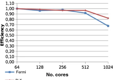
Figure 1.ASHEE parallel efficiency on Fermi and PLX supercom-puters at CINECA (www.cineca.it).
Concerning point 5, it is worth remarking that, according to Ferry et al. (2003), the first-order termτj in Eq. (15) must
be limited to avoid the divergence of preferential concentra-tion in a turbulent flow field (and to keep the effective Stokes number below 0.2). In other words, we impose at each time step that|vj−wj| ≤0.2|ug+wj|. We test the effect of this
limiter on preferential concentration in Sect. 4.2. 3.3 Parallel performances
Figure 1 reports the parallel efficiency of the numerical tests described in Sect. 4.1, on both the Fermi and the PLX (a Linux cluster based on Intel Xeon ESA- and quad-core processors @2.4 GHz) machines at CINECA. The ASHEE code efficiency is very good (above 0.9) up to 512 cores (i.e., up to about 30 000 cells core−1), but it is overall satisfactory for 1024 cores, with efficiency larger than 0.8 on PLX and slightly lower (about 0.7) on Fermi probably due to the lim-ited level of cache optimization and input/output scalability (Culpo, 2011). The code was run also on 2048 cores on Fermi with parallel efficiency of 0.45 (Dagna, 2013).
4 Model verification and evaluation
Evaluation tests are focused on the dynamics of gas (Sect. 4.1) and multiphase (Sect. 4.2) turbulence and on the mixing properties of buoyant plumes (Sect. 4.3). Compress-ibility likely exerts a controlling role to the near-vent dynam-ics during explosive eruptions (e.g., Carcano et al., 2013). Although this is not the focus of this work, we briefly dis-cuss in Sect. 4.4 the performance of the model on a standard one-dimensional shock wave numerical test.
4.1 Compressible decaying homogeneous and isotropic turbulence
Turbulence is a key process controlling the dynamics of vol-canic plumes since it controls the rate of mixing and air en-trainment. To assess the capability of the developed model to resolve turbulence (which requires low numerical diffu-sion and controlled numerical errors; Geurts and Fröhlich, 2002), we have tested the numerical algorithm against differ-ent configurations of decaying homogeneous and isotropic turbulence (DHIT).
In this configuration, the flow is initialized in a domain which is a box with sideL=2π with periodic boundary conditions. As described in Blaisdell et al. (1991), Honein and Moin (2004), Pirozzoli and Grasso (2004), Lesieur et al. (2005) and Liao et al. (2009), we chose the initial velocity field so that its energy spectrum is
E(k)=16 3
r 2 π
urms k0
k
k0 4
e− 2k2
k20 , (25)
with peak initially in k=k0 and so that the initial kinetic energy and enstrophy are
K0= ∞ Z
0
E(k)dk=1 2u
2
rms (26)
H0= ∞ Z
0
k2E(k)dk=58u2rmsk02. (27)
As reviewed by Pope (2000), the Taylor microscale can be written as a function of the dissipationε=2νH:
λ2T≡5νu 2 rms
ε =
5K
H, (28)
thus in our configuration, the initial Taylor microscale is
λT,0= s
5K0 H0 =
2
k0. (29)
We have chosen the non-dimensionalization keeping the root mean square of the magnitude of velocity fluctuations (u′) equal tourms:
urms≡
D√ u′·u′E
≡
1 (2π )3
Z
√
u′·u′dx=2 ∞ Z
0
E(k)dk. (30) We also chose to make the system dimensionless by fixing ρm,0=1,T0=1,Pr=1, so that the ideal gas law becomes
p=ρmRmT =Rm, (31)
and the initial Mach number of the mixture based on the ve-locity fluctuations reads
Marms= s
u2rms cm2 =
s 2K0ρm
γmp =
urms(γmp)− 1
This means that Marms can be modified keeping fixedurms and modifying p. Following Honein and Moin (2004), we define the eddy turnover time:
τe=
√
3λT urms
. (33)
The initial compressibility ratio C0is defined as the ratio between the kinetic energy and its compressible component Kc:
C0=KKc,0
0 = 1 2(2π )3K
0 Z
p
u′c·u′cdx. (34)
Here,u′cis the compressible part of the velocity fluctuations, so that∇ ·u′= ∇ ·u′cand∇ ∧u′c=0.
The last parameter – i.e., the dynamical viscosity – can be given by fixing the Reynolds number based either onλT,0or k0:
Reλ=
ρmurmsλT,0
√
3µ (35)
Rek0= ρmurms
k0µ
. (36)
It is useful to define the maximum resolved wavenumber on the selected N-cells grid and the Kolmogorov length scale based onRek0. TheyRek0– respectively,
kmax=
N 2 −1
2π
L N
N−1, (37)
η=2π k0Re
−34
k0 . (38)
In order to have a Direct Numerical Simulation (DNS), the smallest spatial scale δ should be chosen in order to have kmaxη >2 (Pirozzoli and Grasso, 2004).
We compare the DNS of compressible decaying homo-geneous and isotropic turbulence with a reference, well-tested numerical solver for DNSs of compressible turbulence by Pirozzoli and Grasso (2004) and Bernardini and Piroz-zoli (2009). For this comparison we fix the following initial parameters: p=Rm=1, γm=1.4, Pr=1, Marms=0.2, C0=0,u2rms=2K0=0.056,k0=4,λT=0.5,τe≃3.6596, µ=5.885846×10⁻⁴,Reλ≃116, Rek0≃100. Thus a grid withN=2563cells giveskmax≃127 andkmaxη=2π, big enough to have a DNS. The simulation has been performed on 1024 cores on the Fermi Blue Gene/Qinfrastructure at Italian CINECA super-computing center (http://www.cineca. it), on which about 5 h are needed to complete the highest-resolution runs (2563cells) up to time t /τe=5.465 (about 3500 time steps). The average computing speed on 1024 Fermi cores is about 1–3 Mcells/s, with the variability as-sociated with the number of solid phases described by the model. This value is confirmed in all benchmark cases pre-sented in this paper.
Figure 2.Isosurface atQu≃19 Hz2andt /τe≃2.2, representing
zones with coherent vortices.
k
E(
k)
100 101 102 10-10
10-9 10-8 10-7 10-6 10-5 10-4 10-3 10-2
DNS Bernardini & Pirozzoli
ASHEE
Figure 3. Comparison of a DNS executed with the eight order scheme by Pirozzoli and Grasso (2004) and our code implemented using theC++libraries of OpenFOAM®att /τe=1.093. TheL2 norm between the two spectra is 4.0×10⁻⁴. The main parameters areReλ≃116,Marms=0.2.
Figure 2 shows an isosurface of the second invariant of the velocity gradient, defined as
Qu=
1 2
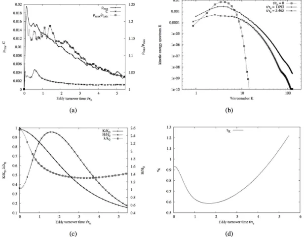
Figure 4. Evolution of dynamical quantities in DHIT withReλ≃116 andMarms=0.2 att /τe=5.465.(a)Density fluctuationsρrms, compressibility C and density contrastρmax/ρmin;(b)evolution of the energy spectrumE(k);(c)non-dimensional kinetic energyK/K0, enstrophyH/H0and Taylor microscaleλT/λT,0;(d)Kolmogorov timescaleτη.
In Fig. 3 we present a comparison of the energy spec-trum E(k)obtained with the ASHEE model and the model by Bernardini and Pirozzoli (2009) after approximatively 1 eddy turnover time; theL2norm of the difference between the two spectra is 4.0×10⁻⁴. This validates the accuracy of our numerical code in the single-phase and shock-free case.
Figure 4 shows the evolution of several integral param-eters describing the dynamics of the decaying homoge-neous and isotropic turbulence. Figure 4a displays the den-sity fluctuations ρrms=ph(ρ− hρi)2i, the density
con-trast ρmax/ρmin and the standard measure of compressibil-ity C= h|∇ ·u|2i/h|∇u|2i which takes value between 0
(incompressible flow) and 1 (potential flow) (Boffetta et al., 2007). All the quantities shown in Fig. 4a depend on the ini-tial Mach number and compressibility. For the case shown,
Marms=0.2 and we obtain very similar results to those re-ported in Figs. 18 and 19 by Garnier et al. (1999).
Figure 4b shows the kinetic energy spectrum at t /τe= 0,1.093,5.465. The energy spectrum widens from the ini-tial condition until its tail reachesk≃kmax≃127. Then the system dissipates and the maximum of the energy spectrum decreases. The largest scales tend to lose energy more slowly
than the other scales and the spectrum widens also in the larger-scale direction.
Table 1.Stokes time, maximum Stokes number and diameter of the solid particles inserted in the turbulent box.
τj Stmax=τj/0.6 dj (ρˆj=103)
0.60 1.0 2.521×10⁻³ 0.30 0.5 1.783×10⁻³ 0.15 0.25 1.261×10⁻³ 0.075 0.125 8.914×10⁻⁴ 0.0375 0.0625 6.303×10⁻⁴
In Fig. 4d we show the evolution of the Kolmogorov timescaleτηduring the evolution of the decaying turbulence.
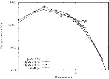
We finally compare in Fig. 5 the DNS described with simulations at lower resolution withN=323cells andN= 643cells. In this case, it is expected that the spectra diverge from the DNS, unless an appropriate subgrid model is intro-duced to simulate the effects of the unresolved to the resolved scales. Several subgrid models have been tested (Cerminara, 2016), both static and dynamic. Figure 5 presents the result-ing spectrum usresult-ing the dynamic WALE model (Nicoud and Ducros, 1999; Lodato et al., 2009). In this figure, we notice how the dynamic WALE model works pretty well for both the 323and 643LES, avoiding the smallest scales to accu-mulate unphysical energy.
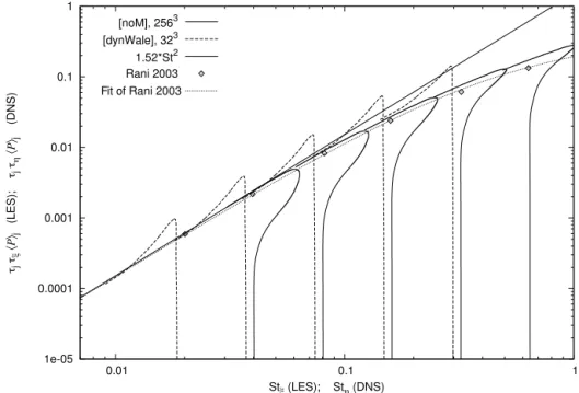
4.2 Multiphase isotropic turbulence
In this section we test the capability of ASHEE to cor-rectly describe the decoupling between solid and gaseous phases whenStj<0.2 and to explore its behavior when the
equilibrium–Eulerian hypothesisStj<0.2 is not fulfilled so
that a limiter to the relative velocityug−uj is applied. We
mainly refer to Rani and Balachandar (2003) for a quantita-tive assessment of numerical model results.
To this aim, we performed a numerical simulation of ho-mogeneous and isotropic turbulence with a gas phase ini-tialized with the same initial and geometric conditions de-scribed in Sect. 4.1. We added to that configuration five solid particle classes chosen in such a way that Stj∈ [0.03,1],
homogeneously distributed and with zero relative velocity: vj(x,0)=0. From Fig. 4d, we see that, during turbulence
decay, approximately τη∈ [0.6,1.2]. Therefore, for a given
particle class with τj fixed, during the time intervalt /τe∈
[0,5.5]we haveStmax/Stmin≃2. In Table 1 we report the main properties of the particles inserted in the turbulent box. To evaluate the Stokes time here we usedτj = ˆρjdj2/(18µ)
because in the absence of settling, Rej <1 when Stj<1
(Balachandar, 2009). We set the material density of all the particles toρˆj=103. In order to have a small contribution of
the particle phases to the fluid dynamics – one way coupling – here we set the solid particle mass fraction to a small value, yj=0.002, so thatyg=0.99.
1e-06 1e-05 0.0001 0.001
1 10
Energy spectrum E(k)
Wavenumber k [noM] 2563
[dynWale] 643 [dynWale] 323 [noM] 323
Figure 5. Energy spectrum E(k) at t /τe=5.465 obtained with different spatial resolutions and with/without subgrid-scale LES model.
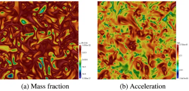
In Fig. 6 we show a slice of the turbulent box att /τe≃2.2. Panel (a) displays the solid mass fraction, highlighting the preferential concentration and clustering of particles in re-sponse to the development of the acceleration field (panel b) associated with turbulent eddies.
As described in Maxey (1987) and Rani and Balachandar (2003), a good measure for the degree of preferential concen-tration in incompressible flows is the weighted average on the particle mass fraction of the quantity(|D|2− |S|2), whereS is the vorticity tensor – i.e., the skew-symmetric part of the gas velocity gradient – and Dis its symmetrical part. For compressible flows, we choose to consider
hPij≡ h|D|2− |S|2− |Tr(D)|2ij≡h
yj(P− hPi)i
hyji
. (40) This is a good measure because (use integration by parts, the Gauss theorem and Eq. 15) withwj =0,
h∇ ·uji= −τj
* X
l,m
(∂lum∂mul−∂lul∂mum)
+
= −τj
D
|D|2− |S|2− |Tr(D)|2E
. (41)
Moreover, it is worth noting thathPij vanishes in the
ab-sence of preferential concentration. By dimensional analysis, preferential concentration is expected to behave as
hPij∝
τj/τη3 DNS
τj/τξ3 LES, (42)
because it must be proportional toτj and have a dimension
Figure 6.Slice of the turbulent box att /τe≃2.2. The two panels represent respectively a logarithmic color map ofy3(Stmax=0.5) and of
|ag|.
corresponding to an eddy length scale ξ in the inertial sub-range, can be evaluated by means of the Kolmogorov’s the-ory as
τξ=τλ
ξ
λT 2
3
, (43)
where the Taylor microscaleλTis defined by Eq. (28). Since the time based on the Taylor microscale is defined as
τλ= √
3λT
urms , (44)
we can evaluate the typical time at the smallest resolved LES scaleξ knowing the kinetic energyK(t )andλT(t ):
τξ(t )=
s 3 2K(t )ξ
2
3λT(t )13. (45)
In Fig. 7 we show the time evolution of the degree of pref-erential concentration as a function of the Stokes number for both DNS with 2563cells and the LES with 323cells. There, we multiplyhPij byτξτj in order to make it dimensionless
and to plot on the same graph all the different particles at different times together.
At t=0 the preferential concentration is zero for all Stokes numbers. Then, preferential concentration of each particle class increases up to a maximum value and then it de-creases because of the decaying of the turbulent energy. The maximum degree of preferential concentration is reached by each particle class whenτη is minimum (att /τe≃1.7, see Fig. 4d). Then, hPij decreases and merges with the curve relative to the next particle class at the final simulation time, whenτη is about twice its minimum. Note that the expected
behavior of Eq. (42) is reproduced forStj<0.2 and in
par-ticular we find
hPij≃
(
1.52Stjτη−2 DNS
1.52Stjτξ−2 LES. (46)
Moreover, by comparing our results with the Eulerian– Lagrangian simulation described in Rani and Balachandar (2003), we note that our limiter for the preferential concen-tration whenSt>0.2 is well behaving.
For the sake of completeness, we found that the best fit in the rangeSt<2.5 for the data found by Rani and Balachan-dar (2003) is
hPij≃1.52× Stj
1+3.1×Stj+3.8×St2j
τη−2, (47)
with root mean square of residuals 8.5×10⁻³.
Regarding the 323LES simulation, Fig. 7 shows that the Stokes number of each particle class in the LES case is much smaller than its DNS counterpart. In accord with Balachan-dar and Eaton (2010), we have
Stξ=Stη
η
ξ 2
3
, (48)
1e-05 0.0001 0.001 0.01 0.1 1
0.01 0.1 1
τj τξ
〈
P
〉j
(LES);
τj τη
〈
P
〉j
(DNS)
Stξ (LES); Stη (DNS) [noM], 2563
[dynWale], 323 1.52*St2 Rani 2003 F
it of Rani 2003
Figure 7. Evolution of the degree of preferential concentration withStξ (LES) orStη (DNS). We obtain a good agreement between
equilibrium–Eulerian LES/DNS and Lagrangian DNS simulations. The fit for the data by Rani and Balachandar (2003) is found in Eq. (47).
4.3 Turbulent forced plume
As a third benchmark, we discuss high-resolution, three-dimensional numerical simulation of a forced gas plume, produced by the injection of a gas flow from a circular in-let into a stable atmospheric environment at lower tempera-ture (and higher density). Such an experiment allows us to test the numerical model behavior against some of the funda-mental processes controlling volcanic plumes, namely den-sity variations, non-isotropic turbulence, mixing, air entrain-ment and thermal exchange. This study is mainly aimed at assessing the capability of the numerical model to describe the time-average behavior of a turbulent plume and to repro-duce the magnitude of large-scale fluctuations and large-eddy structures. We will mainly refer to laboratory experiments by George et al. (1977) and Shabbir and George (1994) and nu-merical simulations by Zhou et al. (2001) for a quantitative assessment of model results.
Numerical simulations describe a vertical round forced plume with heated air as the injection fluid. The plume axis is aligned with the gravity vector and is subjected to a positive buoyancy force. The heat source diameter 2b0 is 6.35 cm, the exit vertical velocity on the axis u0 is 0.98 m s−1, the inflow temperatureT0is 568 K and the ambient air temper-ature Tα is 300 K. The corresponding Reynolds number is
1273, based on the inflow mean velocity, viscosity and di-ameter. Air properties at inlet are Cp=1004.5 J(K kg)−1,
R=287 J(K kg)−1andµ=3×10⁻⁵Pa s.
As discussed by Zhou et al. (2001) the development of the turbulent plume regime is quite sensitive to the inlet
condi-tions: we therefore tested the model by adding a periodic per-turbation and a non-homogeneous inlet profile to anticipate the symmetry breaking, and the transition from a laminar to a turbulent flow. The radial profile of vertical velocity has the form
u(r)=1 2u0
1−tanh
b 0 4δr
r
b0− b0
r
, (49)
whereδr is the thickness of the turbulent boundary layer at
the plume inlet, that we have set atδr=0.1b0. A periodical
forcing and a random perturbation of intensity 0.05u0 has been superimposed to mimic a turbulent inlet.
The resulting average mass, momentum and buoyancy flux areQ0=2.03×10⁻³kg s−1,M0=1.62×10⁻³kg m s−2and F0=1.81×10⁻³kg s−1.
The computational grid is composed of 360×180×180 uniformly spaced cells (deformed near the bottom plane to conform to the circular inlet) in a box of size 12.8×6.4×6.4 diameters. In particular, the inlet is discretized with 400 cells. The adaptive time step was set to keep theCo<0.2. Based on estimates by Plourde et al. (2008), the selected mesh refinement is coarser than the required grid to fully re-solve turbulent scales in a DNS (which would require about 720×360×360 cells). Nonetheless, this mesh is resolved enough to avoid the use of a subgrid-scale model. This can be verified by analyzing the energy spectra of fluctuations on the plume axis and at the plume outer edges. In Fig. 8 we show the energy spectra of temperature and pressure as a func-tion of the non-dimensional frequency: the Strouhal number
a result similar to Plourde et al. (2008), where the inertial– convective regime with the decay −5/3 and the inertial– diffusive regime with the steeper decay −3 are observable (List, 1982).
Model results describe the establishment of the turbulent plume through the development of fluid-dynamic instabili-ties near the vent (puffing is clearly recognized as a toroidal vortex in Fig. 9a). The breaking of large-eddies progressively leads to the onset of the developed turbulence regime – which is responsible for the mixing with the surrounding ambient air, radial spreading of the plume and decrease of the plume average temperature and velocity. Figure 9a displays the spa-tial distribution of gas temperature. Mixing becomes effec-tive above a distance of about four diameters. Figure 9b dis-plays the distribution of the vorticity, represented by values of the Qu invariant (Eq. 39). The figure clearly identifies
the toroidal vortex associated with the first instability mode (puffing, dominant at such Reynolds numbers). We observed the other instability modes (helical and meandering; Lesieur et al., 2005) only by increasing the forcing intensity (not shown).
Experimental observations by George et al. (1977) and Shabbir and George (1994) reveal that the behavior of forced plumes far enough from the inlet can be well described by integral one-dimensional plume models (Morton et al., 1956; Morton, 1959) provided that an adequate empirical entrain-ment coefficient is used. In the buoyant plume regime at this Reynolds number George et al. (1977) obtained an entrain-ment coefficient of 0.153.
To compare numerical result with experimental observa-tions and one-dimensional average plume models, we have time-averaged the numerical results between 4 and 10 s (when the turbulent regime was fully developed) and com-puted the vertical mass Q(z), momentum M(z)and buoy-ancyF (z)fluxes as a function of the height. To perform this operation, we define the time-averaging operation(¯·)and the horizontal domain:
O(z)= {(x, y)∈R2|(ytracer(x) >0.01
×ytracer,0)∧(uz(x) >0)}, (50)
where(x, y, z)=x are the spatial coordinates,ytracer is the mass fraction field of a tracer injected from the vent with ini-tial mass fractionytracer,0anduzis the axial component of the
velocity field. We use this definition forO(z)for coherence with integral plume models, where the mean velocity field is assumed to have the same direction as the plume axis (see Morton et al., 1956; Woods, 1988; Cerminara, 2015, 2016; Cerminara et al., 2016). This hypothesis is tested in Fig. 10a, where it can be verified that the time-averaged streamlines inside the plume are parallel to the axis (Fig. 10b shows the instantaneous streamlines and velocity magnitude field).
The plume fluxes are evaluated as follows (see George et al., 1977; Shabbir and George, 1994; Kaminski et al., 2005):
– mass fluxQ(z)=ROρ uzdxdy,
– momentum fluxM(z)=ROρ u2zdxdy, – buoyancy fluxF (z)=ROuz(ρα−ρ)dxdy,
where ρα=ρα(z) is the atmospheric density. From these
quantities it is possible to retrieve the main plume parame-ters:
– plume radiusb(z)= q
Q(F+Q) π ραM ,
– plume densityβ(z)=ρα (FQ+Q),
– plume temperatureTβ(z)=TαF+QQ,
– plume velocityU (z)=MQ,
– entrainment coefficientκ(z)=2π ραU bQ′ ,
where(·)′is the derivative along the plume axis andTαis the
atmospheric temperature profile.
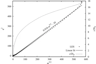
Figure 11 displays the average plume radius and veloc-ity. As previously reported by Fanneløp and Webber (2003) and Plourde et al. (2008), the plume radius initially shrinks due to the sudden increase of velocity due to buoyancy (at z=0.1 m). Above, turbulent mixing becomes effective and increases the plume radius while decreasing the average ve-locity. The upper inset in Fig. 11 shows the values of the vertical massq=Q/Q0, momentumm=M/M0and buoy-ancyf=F /F0, normalized with the inlet values. All vari-ables have the expected trends and, in particular, the buoy-ancy flux is constant (as expected for weak ambient stratifica-tion) whereasq andmmonotonically increase and attain the theoretical asymptotic trends shown also in Fig. 12. Indeed, Fanneløp and Webber (2003) have shown that an integral plume model for non-Boussinesq regimes (i.e., large density contrasts) in the approximation of weak ambient stratifica-tion and adopting the Ricou and Spalding (1961) formula-tion for the entrainment coefficient, has a first integral such that q2 is proportional to m5/2 at all elevations. Figure 12 demonstrates that this relationship is well reproduced by our numerical simulations, as also observed in DNS by Plourde et al. (2008).
The lower inset in Fig. 11 shows the computed entrain-ment coefficient, which is very close to the value found in experiments (George et al., 1977; Shabbir and George, 1994) and numerical simulations (Zhou et al., 2001) of an anal-ogous forced plume. We found a value around 0.14 in the buoyant plume region (6.4< z/2b0<16).
Figure 8.Temperature (solid) and pressure (dashed) fluctuations energy spectra:(a)at a point along the plume axis (0, 0, 0.5715) m;(b)at a point along the plume outer edge (0, 0.06858, 0.5715) m. The slopesStr−5/3andStr−3are represented with a thick solid and dashed line respectively.
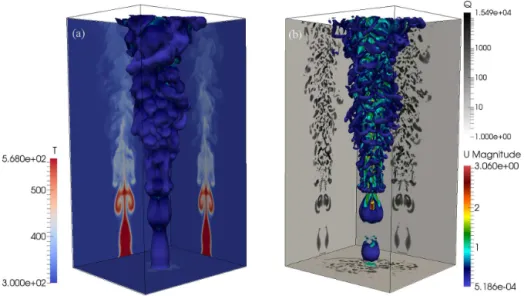
Figure 9. Three-dimensional numerical simulation of a forced gas plume att=10 s.(a)Isosurface of temperatureT =305 K, colored with the magnitude of velocity, and the temperature distribution on two orthogonal slices passing across the inlet center.(b)Isosurface of Qu=100 s−2colored with the value of the velocity magnitude, and its distribution across two vertical slices passing through the inlet center.
uz(x, y)=Ufitexp −
x2+y2 bfit2
!
. (51)
The slope of the function bfit(z) has been evaluated in the region 6.4< z/2b0<16, to obtain bfit/z=0.142±0.001 to be compared with the result of George et al. (1977): bfit/z=0.135±0.010.
Finally, Fig. 14 reports the time-averaged values of the vertical velocity and temperature along the plume axis. As observed in laboratory experiments, velocity is slightly in-creasing and temperature is almost constant up to above four inlet diameters, before the full development of the turbu-lence. When the turbulent regime is established, the decay of the velocity and temperature follows the trends predicted by the one-dimensional theory and observed in experiments.
The inset displays the average value of the vertical veloc-ity and temperature fluctuations along the axis. Coherently with experimental results (George et al., 1977), velocity fluc-tuations reach their maximum value and a stationary trend (corresponding to about 30 % of the mean value) at a lower height (about three inlet diameters) with respect to tempera-ture fluctuations (which reach a stationary value about 40 % above four inlet diameters).
4.4 Transonic and supersonic flows
describ-Figure 10.Two-dimensional slice and streamlines of the velocity field:(a)time-averaged velocity field;(b)instantaneous velocity field at t=10 s. The mean velocity field outside the plume is approximatively horizontal while in the plume it is approximately vertical. The region where the mean velocity field change direction is the region where the entrainment of air by the plume occurs.
0 0.2 0.4 0.6 0.8 1
0 0.5 1 1.5 2
0 0.1 0.2 0.3 0.4 0.5
H eight [m]
P
lume velocity [m/s] P
lume radius [m]
plume radius plume velocity
0 0.2 0.4 0.6 0.8 1
0 2 4 6 8 10 12 14 q m f
0 0.2 0.4 0.6 0.8 1
0 0.05 0.1 0.15 0.2 entrainment k = 0.141±0.001
Figure 11.Time-averaged plume radius and velocity. The insets display the non-dimensional mass, momentum and buoyancy fluxes (top) and the time-averaged entrainment coefficient. The line in the entrainment panel is a constant fit, from which resultsκ=0.141±0.001.
ing the expansion of a compressible, single-phase gas hav-ing adiabatic index γ=1.4. At t=0 the domain of length 10 m is subdivided into two symmetric subsets. In the first subset (spatial coordinatex <0) we setu=0, p=105Pa,