ASHEE: a compressible, Equilibrium–Eulerian model for volcanic ash plumes

(1)

GMDD

8, 8895–8979, 2015

An equilibrium Eulerian model for

volcanic plumes

M. Cerminara et al.

Title Page

Abstract Introduction

Conclusions References

Tables Figures

◭ ◮

Back Close

Full Screen / Esc

Printer-friendly Version Interactive Discussion

Discussion

P

a

per

|

Discussion

P

a

per

|

Discussion

P

a

per

|

Discussion

P

a

per

|

Geosci. Model Dev. Discuss., 8, 8895–8979, 2015 www.geosci-model-dev-discuss.net/8/8895/2015/ doi:10.5194/gmdd-8-8895-2015

This discussion paper is/has been under review for the journal Geoscientific Model Development (GMD). Please refer to the corresponding final paper in GMD if available.

ASHEE: a compressible,

Equilibrium–Eulerian model for volcanic

ash plumes

M. Cerminara1,2, T. Esposti Ongaro2, and L. C. Berselli3

1

Scuola Normale Superiore, Pisa, Italy

2

Istituto Nazionale di Geofisica e Vulcanologia, Sezione di Pisa, Pisa, Italy

3

Dipartimento di Matematica, Università degli Studi di Pisa, Pisa, Italy

Received: 4 September 2015 – Accepted: 20 September 2015 – Published: 19 October 2015

Correspondence to: M. Cerminara (matteo.cerminara@ingv.it)

(2)

GMDD

8, 8895–8979, 2015

volcanic plumes

M. Cerminara et al.

Title Page

Tables Figures

◭ ◮

Back Close

Full Screen / Esc

Discussion

P

a

per

|

Discussion

P

a

per

|

Discussion

P

a

per

|

Discussion

P

a

per

|

Abstract

A new fluid-dynamic model is developed to numerically simulate the non-equilibrium dynamics of polydisperse gas-particle mixtures forming volcanic plumes. Starting from the three-dimensional N-phase Eulerian transport equations (Neri et al., 2003) for a mixture of gases and solid dispersed particles, we adopt an asymptotic expansion

5

strategy to derive a compressible version of the first-order non-equilibrium model (Ferry and Balachandar, 2001), valid for low concentration regimes (particle volume fraction less than 10−3) and particles Stokes number (St, i.e., the ratio between their relaxation time and flow characteristic time) not exceeding about 0.2. The new model, which is called ASHEE (ASH Equilibrium Eulerian), is significantly faster than the N-phase

10

Eulerian model while retaining the capability to describe gas-particle non-equilibrium

eﬀ_{ects. Direct numerical simulation accurately reproduce the dynamics of isotropic,}

compressible turbulence in subsonic regime. For gas-particle mixtures, it describes the main features of density fluctuations and the preferential concentration and cluster-ing of particles by turbulence, thus verifycluster-ing the model reliability and suitability for the

15

numerical simulation of high-Reynolds number and high-temperature regimes in pres-ence of a dispersed phase. On the other hand, Large-Eddy Numerical Simulations of forced plumes are able to reproduce their observed averaged and instantaneous flow properties. In particular, the self-similar Gaussian radial profile and the development of large-scale coherent structures are reproduced, including the rate of turbulent mixing

20

and entrainment of atmospheric air. Application to the Large-Eddy Simulation of the injection of the eruptive mixture in a stratified atmosphere describes some of important features of turbulent volcanic plumes, including air entrainment, buoyancy reversal, and

maximum plume height. For very fine particles (St_→0, when non-equilibrium eﬀ_ects

are negligible) the model reduces to the so-called dusty-gas model. However, coarse

25

particles partially decouple from the gas phase within eddies (thus modifying the tur-bulent structure) and preferentially concentrate at the eddy periphery, eventually being

(3)

mech-GMDD

8, 8895–8979, 2015

volcanic plumes

M. Cerminara et al.

Title Page

Tables Figures

◭ ◮

Back Close

Full Screen / Esc

Discussion

P

a

per

|

Discussion

P

a

per

|

Discussion

P

a

per

|

Discussion

P

a

per

|

anisms, gas-particle non-equilibrium processes are able to influence the large-scale behavior of volcanic plumes.

1 Introduction

Explosive volcanic eruptions are characterized by the injection from a vent into the at-mosphere of a mixture of gases, liquid droplets and solid particles, at high velocity and

5

temperature. In typical magmatic eruptions, solid particles constitute more than 95 % of the erupted mass and are mostly produced by the brittle fragmentation of a highly viscous magma during its rapid ascent in a narrow conduit (Wilson, 1976; Sparks, 1978), with particle sizes and densities spanning over a wide range, depending on the overall character and intensity of the eruption (Kaminski and Jaupart, 1998; Kueppers

10

et al., 2006). The order of magnitude of the plume mixture volumetric concentration very rarely exceedǫs∼3×10−

3

, because the order of magnitude of the ejected frag-ments density is ˆρs∼10

3

kg m−3. Thus, the plume mixture con be considered mainly

as a dilute suspension in the sense of Elghobashi (1991, 1994). This threshold forǫs

is overcome in the dense layer forming in presence of pyroclastic density currents (see

15

e.g. Orsucci, 2014). In the literature, collisions between ash particles are usually dis-regarded when looking at the dynamics of volcanic ash plume, because this dilute character of the plume mixture (cf. Morton et al., 1956; Woods, 2010).

After injection in the atmosphere, this multiphase eruptive mixture can rise convec-tively in the atmosphere, forming either a buoyant volcanic plume or collapse

catas-20

trophically forming pyroclastic density currents. Since these two end-members have diﬀ_{erent spatial and temporal scales and di}ﬀ_{erent impacts on the surrounding of a}

vol-cano, understanding the dynamics of volcanic columns and the mechanism of this bifurcation is one of the topical aims of volcanology and one of the main motivations for this work.

25

The term volcanic columnwill be adopted in this paper to generically indicate the

(4)

GMDD

8, 8895–8979, 2015

volcanic plumes

M. Cerminara et al.

Title Page

Tables Figures

◭ ◮

Back Close

Full Screen / Esc

Discussion

P

a

per

|

Discussion

P

a

per

|

Discussion

P

a

per

|

Discussion

P

a

per

|

nomenclature, we will term jet the inertial regime of the volcanic column and plume

the buoyancy-driven regime. Aforced plumeis characterized by an initial

momentum-driven jet stage, transitioning into a plume.

In this work, we present a new computational fluid-dynamic model to simulate tur-bulent gas-particle forced plumes in the atmosphere. Although the focus of the paper

5

is on multiphase turbulence in subsonic regimes, the model is also suited to be ap-plied to transonic and supersonic flows. In many cases, indeed, the eruptive mixture is injected in the atmosphere at pressure higher than atmospheric, so that the flow is initially driven by a rapid, transonic decompression stage. This is suggested by nu-merical models predicting choked flow conditions at the volcanic vent (Wilson, 1980;

10

Wilson et al., 1980), implying a supersonic transition above the vent or in the crater

(Kieﬀ_{er, 1984; Woods and Bower, 1995; Koyaguchi et al., 2010) and it is supported by}

field evidences of the emission of shock waves during the initial stages of an eruptions (Morrissey, 1997). Despite the importance of the decompression stage for the subse-quent development of the volcanic plume (Pelanti and LeVeque, 2006; Ogden et al.,

15

2008b; Orescanin et al., 2010; Carcano et al., 2013) and for the stability of the eruptive column (Ogden et al., 2008a), our analysis is limited to the plume region where flow pressure is equilibrated to the atmospheric pressure. From laboratory experiments, this is expected to occur within less than 20 inlet diameters above the ground (Yüceil and Ötügen, 2002).

20

1.1 Dusty gas modeling of volcanic plumes

Starting from the assumption that the large-scale behavior of volcanic columns is

con-trolled by thebulk properties of the eruptive mixture, most of the previous models of

volcanic plumes have considered the eruptive mixture as homogeneous (i.e., they as-sume that particles are perfectly coupled to the gas phase). Under such hypothesis,

25

the multiphase transport equations can be largely simplified and reduce to a set of

mass, momentum and energy balance equations for a single fluid (nameddusty-gasor

(5)

veloc-GMDD

8, 8895–8979, 2015

volcanic plumes

M. Cerminara et al.

Title Page

Tables Figures

◭ ◮

Back Close

Full Screen / Esc

Discussion

P

a

per

|

Discussion

P

a

per

|

Discussion

P

a

per

|

Discussion

P

a

per

|

ity and temperature) and equation of states accounting for the incompressibility of the particulate phase and gas covolume (Marble, 1970).

By adopting the dusty gas approximation, volcanic plumes have been studied in the framework of jet (Prandtl, 1963) and plume theory (Morton et al., 1956; Morton, 1959). One-dimensional, steady-state pseudo-gas models of volcanic plumes have thus had

5

a formidable role in volcanology to identify the main processes controlling their dynam-ics and scaling properties (Wilson, 1976; Woods, 1988; Sparks et al., 1997).

Accordingly, volcanic plume dynamics is schematically subdivided into two main stages. The lower, jet phase is driven by the initial flow momentum. Mixture buoyancy is initially negative (the bulk density is larger than atmospheric) but the mixture

pro-10

gressively expands adiabatically thanks to atmospheric air entrainment and heating, eventually undergoing a buoyancy reversal. When buoyancy reversal does not occur, partial or total collapse of the jet from its maximum thrust height (where the jet has lost all its initial momentum) and generation of pyroclastic density currents are expected.

Above the jet thrust region, the rise of volcanic plumes is driven by buoyancy and

15

it is controlled by turbulent mixing until, in the stratified atmosphere, a level of neutral buoyancy is reached. Above that height, the plume starts to spread out achieving its maximum height and forming an umbrella ash cloud, dispersing in the atmosphere and slowly falling-out.

In one-dimensional, time-averaged models, entrainment of atmospheric air is

de-20

scribed by one empirical coeﬃ_{cient (the entrainment coe}ﬃ_{cient) relating the influx of}

atmospheric air to the local, vertical plume velocity. The entrainment coeﬃ_{cient also}

determines the plume shape (Ishimine, 2006) and can be empirically determined by means of direct field observations or ad-hoc laboratory measurements.

Further development of volcanic plume models have included the influence of

atmo-25

spheric stratification and humidity (Woods, 1993; Glaze and Baloga, 1996), the eﬀ_ect

of cross wind (Bursik, 2001), loss and reentrainment of solid particles from plume

mar-gins (Woods and Bursik, 1991; Veitch and Woods, 2002), and transient eﬀ_{ects (Scase,}

(6)

GMDD

8, 8895–8979, 2015

volcanic plumes

M. Cerminara et al.

Title Page

Tables Figures

◭ ◮

Back Close

Full Screen / Esc

Discussion

P

a

per

|

Discussion

P

a

per

|

Discussion

P

a

per

|

Discussion

P

a

per

|

the self-similarity hypothesis, whose validity cannot be experimentally ascertained for volcanic eruptions.

To overcome the limitations of one-dimensional models, three-dimensional dusty-gas models have been developed to simulate volcanic plumes. Suzuki (2005) have developed a three-dimensional dusty gas model (SK-3-D) able to accurately resolve the

5

relevant turbulent scales of a volcanic plume, allowing a first, theoretical determination

of the entrainment coeﬃ_{cient (Suzuki and Koyaguchi, 2010), without the need of an}

empirical calibration.

To simulate the three-dimensional large-scale dynamics of volcanic plumes including particle settling and the complex microphysics of water in volcanic plumes, the ATHAM

10

(Active Tracer High Resolution Atmospheric Model) code has been designed (Ober-huber et al., 1998; Graf et al., 1999; Van Eaton et al., 2015). ATHAM describes the dynamics of gas-particle mixtures by assuming that particles are in kinetic equilibrium with the gas phase only in the horizontal component, whereas along the vertical

direc-tion they are allowed to have a diﬀ_{erential velocity. Thermal equilibrium is assumed.}

15

In this sense, ATHAM relaxes the dusty-gas approximation (while maintaining its fun-damental structure and the same momentum transport equations) by describing the settling of particles with respect to the gas.

1.2 Multiphase flow models of volcanic plumes

Notwithstanding all the above advantages, dusty-gas models are still limited by the

20

equilibrium assumption, which can be questionable at least for the coarsest part of the granulometric spectrum in a plume. Turbulence is indeed a non-linear, multiscale process and the time and space scales of gas-particle interaction may be compara-ble with some relevant turbulent scales, thus influencing the large-scale behavior of volcanic plumes.

25

(7)

GMDD

8, 8895–8979, 2015

volcanic plumes

M. Cerminara et al.

Title Page

Tables Figures

◭ ◮

Back Close

Full Screen / Esc

Discussion

P

a

per

|

Discussion

P

a

per

|

Discussion

P

a

per

|

Discussion

P

a

per

|

Valentine and Wohletz (1989) and Dobran et al. (1993); Neri and Dobran (1994) have first analyzed the influence of erupting parameters on the column behavior to identify: by means of two-dimensional numerical simulations, they individuate a threshold from collapsing to convective columns. Lately, two-dimensional (Di Muro et al., 2004; Dartev-elle et al., 2004) and three-dimensional numerical simulations (Esposti Ongaro et al.,

5

2008) has contributed to modify the view of a sharp transition between convecting and collapsing columns in favor of that of a transitional regime, characterized by a pro-gressively increasing fraction of mass collapsing. However, previous works could not investigate in detail the non-equilibrium eﬀ_{ects in volcanic plumes, mainly because of}

their averaged description of turbulence: a detailed resolution of the relevant turbulent

10

scales in three dimensions would indeed be computationally prohibitive for N-phase systems.

The main objective of the present work is therefore to develop a new physical model and a fast three-dimensional numerical code able to resolve the spatial and tempo-ral scales of the interaction between gas and particles in turbulent regime and to

15

describe the kinetic non-equilibrium dynamics and their influence on the observable

features of volcanic plumes. To this aim, a development of the so-calledEquilibrium–

Eulerianapproach (Ferry and Balachandar, 2001; Balachandar and Eaton, 2010) has been adopted. It is a generalization of the dusty-gas model keeping the kinematic non-equilibrium as a first order correction of the Marble (1970) model with respect to the

20

Stokes number of the solid particles/bubbles in the mixture. Here, we generalize the Ferry and Balachandar (2001) model to the compressible two-way case.

The derivation of the fluid dynamic model describing the non-equilibrium gas-particle mixture is described in detail in Sect. 2. The computational solution procedure and the numerical code development are reported in Sect. 3. Section 4 focuses on verification

25

(8)

GMDD

8, 8895–8979, 2015

volcanic plumes

M. Cerminara et al.

Title Page

Tables Figures

◭ ◮

Back Close

Full Screen / Esc

Discussion

P

a

per

|

Discussion

P

a

per

|

Discussion

P

a

per

|

Discussion

P

a

per

|

plumes and discusses some aspects related to numerical grid resolution in practical cases.

2 The multiphase flow model

To derive an appropriate multiphase flow model to describe gas-particle volcanic plumes, we here introduce the non-dimensional scaling parameters characterizing gas

5

particle and particle particle interactions.

The drag force between gas and particles introduces in the system a time scale

τs, theparticle relaxation time, which is the time needed to a particle to equilibrate to

a change of gas velocity. Gas-particle drag is a non-linear function of the local flow vari-ables and, in particular, it depends strongly on the relative Reynolds number, defined

10

as:

Res=

ˆ

ρg|us−ug|ds

µ (1)

hereds is the particle diameter, ˆρgis the gas density, µis the gas dynamic viscosity

coeﬃ_{cient and} _u

g(s) is the gas (solid) phase velocity field. Being ˆρg(s) the gaseous

(solid) phase density andǫs=Vs/V the volumetric concentration of the solid phase, it

15

is useful to define the gas bulk densityρg≡(1−ǫs) ˆρg≃ρˆg and the solid bulk density

ρs≡ǫsρˆs (even though in our applicationsǫsis order 10− 3

,ρs is non-negligible since

ˆ

ρs/ρˆgis of order 10 3

).

For an individual point-like particle (i.e., having diameter ds much smaller than the

scale of the problem under analysis), atRes<1000, the drag force per volume unity

20

can be given by the Stokes’ law:

fs=

ρs

τs

(9)

GMDD

8, 8895–8979, 2015

volcanic plumes

M. Cerminara et al.

Title Page

Tables Figures

◭ ◮

Back Close

Full Screen / Esc

Discussion

P

a

per

|

Discussion

P

a

per

|

Discussion

P

a

per

|

Discussion

P

a

per

|

where

τs≡

ˆ

ρs

ˆ

ρg

ds2

18ν φc(Res)

(3)

is the characteristic time of particle velocity relaxation with respect the gas, ˆρs is the

particle density,νis the gas kinematic viscosity and φc=1+0.15Re 0.687

s is a

correc-tion factor (obtained from the Schiller–Naumann correlacorrec-tion) for finite particle Reynolds

5

number (cf. Clift et al., 1978; Balachandar, 2009; Balachandar and Eaton, 2010; Cer-minara, 2015b). In Eq. (2) we disregard all the eﬀ_{ects due to the pressure gradient, the}

added mass, the Basset history and the Saﬀ_{man terms, because we are considering}

heavy particles: ˆρs/ρˆg≫1 (cf. Ferry and Balachandar, 2001; Bagheri et al., 2013).

Equation (2) has a linear dependence on the fluid-particle relative velocity only when

10

Res≪1, so thatφc≃1 and the classic Stokes drag expression is recovered. On the

other hand, if the relative Reynolds numberResgrows, non-linear eﬀects become much

more important in Eq. (3). The Clift et al. (1978) empirical relationship used in this work has been used and tested in a number of papers (e.g., Balachandar and Eaton, 2010; Wang and Maxey, 1993; Bonadonna et al., 2002), and it is equivalent to assuming the

15

following gas-particle drag coeﬃ_cient:

CD(Res)=

24

Re_s(1+0.15Re 0.687

s ) . (4)

Wang and Maxey (1993) discussed nonlinear eﬀ_{ects due to this correction on the}

dy-namics of point-like particles falling under gravity in an homogeneous and isotropic turbulent surrounding. We recall here the terminal velocity that can be found by setting

20

ug=0 in Eq. (2) is:

w_s=

s

4dsρˆs

3CDρgg g=_τ

(10)

GMDD

8, 8895–8979, 2015

volcanic plumes

M. Cerminara et al.

Title Page

Tables Figures

◭ ◮

Back Close

Full Screen / Esc

Discussion

P

a

per

|

Discussion

P

a

per

|

Discussion

P

a

per

|

Discussion

P

a

per

|

As previously pointed out, correction used in Eq. (4) is valid ifRes<10 3

, the regime addressed in this work for ash particles much denser then the surrounding fluid and

smaller than 1 mm. As shown by Balachandar (2009), maximum values of Re_s are

associated to particle gravitational settling (not to turbulence). Using formula Eqs. (4) and (5), it is thus possible to estimate Res of a falling particle with diameter ds. We

5

obtain that Re_s is always smaller than 103 for ash particles finer than 1 mm in air.

If regimes with a bigger decoupling needs to be explored, more complex empirical

correction has to be used forφc(Neri et al., 2003; Bürger and Wendland, 2001).

The same reasoning can be applied to estimate thethermal relaxation timebetween

gas and particles. In terms of the solid phase specific heat capacityCs and its thermal

10

conductivitykg, we have:

τT =

2

Nu_s

ˆ

ρsCs

kg

ds2

12, (6)

where Nu_s=_Nu

s(Res,Pr) is the Nusselt number, usually function of the relative

Reynolds number and of the Prandtl number of the carrier fluid (Neri et al., 2003).

In terms of τ_T, the heat exchange between a particle at temperature Ts and the

sur-15

rounding gas at temperatureTgper unit volume is:

Q_T =ρsCs

τ_T (Ts−Tg) . (7)

Comparing the kinetic and thermal relaxation times we get:

τT τs

=3

2 2φc Nus

Csµ

kg

. (8)

In order to estimate this number, firstly we notice that factor 2φc/Nus tends to 1 if

20

(11)

GMDD

8, 8895–8979, 2015

volcanic plumes

M. Cerminara et al.

Title Page

Tables Figures

◭ ◮

Back Close

Full Screen / Esc

Discussion

P

a

per

|

Discussion

P

a

per

|

Discussion

P

a

per

|

Discussion

P

a

per

|

2015b). Then, in the case of ash particles in air, we have (in SI units)µ≃10−5,Cs≃

103,kg≃10− 2

. Thus we have thatτ_T/τs≃1, meaning that the thermal equilibrium time

is typically of the same order of magnitude of the kinematic one. This bound is very useful when we write the Equilibrium–Eulerian and the dusty gas models, because it tells us that the thermal Stokes number is of the same order of the kinematic one, at

5

least for volcanic ash finer than 1 mm.

The non-dimensional Stokes number (St) is defined as the ratio between the kinetic

(or thermal) relaxation time and a characteristic time of the flow under investigation

τ_F, namely St_s=_τ

s/τF. The definition of the flow time-scale can be problematic for

high-Reynolds number flows (typical of volcanic plumes), which are characterized by

10

a wide range of interacting length- and time-scales, a distinctive feature of the turbulent

regime. For volcanic plumes, the more energetic time-scale would be of the orderτ_L=

L/U, where L and U are the plume diameter and velocity at the vent, which gives

the characteristic turnover time of the largest eddies in a turbulent plume (e.g., Zhou et al., 2001). On the other hand, the smallest time-scale (largestSts) can be defined

15

by the Kolmogorov similarity law byτ_η_∼τ_LRe−_L1/2, where the macroscopic Reynolds number is defined, at a first instance, byRe_L=_UL/ν_,_ν_{being the kinematic viscosity}

of the gas phase alone. For numerical models, it is also useful introducing the

Large-Eddy Simulation (LES) time-scale τ_ξ, with respect to the resolved scales ξ, related

to the numerical grid resolution, size of the explicit filter, and discretization accuracy

20

(Lesieur et al., 2005; Garnier et al., 2009; Balachandar and Eaton, 2010; Cerminara

et al., 2015). At LES scale ξ, Sts is not as large as at the Kolmogorov scale, thus

the decoupling between particles and the carrier fluid is mitigated by the LES filtering operation. We found thatSts.0.2 for LES of volcanic ash finer than 1 mm.

The model presented here is conceived for resolvingdilutesuspensions, namely

mix-25

tures of gases and particles with volumetric concentration Vs

V ≡ǫs.10− 3

(12)

GMDD

8, 8895–8979, 2015

volcanic plumes

M. Cerminara et al.

Title Page

Tables Figures

◭ ◮

Back Close

Full Screen / Esc

Discussion

P

a

per

|

Discussion

P

a

per

|

Discussion

P

a

per

|

Discussion

P

a

per

|

can also be justified by analyzing the time scale of particle–particle collisions. In the dilute regime, in which we can assume an equilibrium Maxwell distribution of particle velocities, the mean free path of solid particles is given by (Gidaspow, 1994):

λp-p=

1

6√2

ds

ǫs

. (9)

Consequently, particle–particle collisions are relatively infrequent (λp-p∼0.1 m≪ds),

5

so that we can neglect, as a first approximation, particle–particle collisions and con-sider the particulate fluid as pressure-less, inviscid and non-conductive.

In volcanic plumes the particle volumetric concentration can exceed of one order of

magnitude the thresholdǫs≃10−

3

only near the vent (see, e.g., Sparks et al., 1997; Esposti Ongaro et al., 2008). However, the region of the plume where the dilute

sus-10

pension requirement is not fulfilled remains small with respect the size of the entire plume, weakly influencing its global dynamics. Indeed, as we will show in Sect. 5, air entrainment and particle fallout induce a rapid decrease of the volumetric concentra-tion. On the contrary, the mass fraction of the solid particles can not be considered small, because particles are heavy: ǫs×ρˆs≡ρs≃ρg. Thus, particles inertia will be

15

considered in the present model: in other words, we will consider thetwo waycoupling

between dispersed particles and the carrier gas phase.

Summarizing, our multiphase model focuses and carefully takes advantage of the hypotheses characterizing the following regimes: heavy particles ( ˆρs/ρˆg≫1) in dilute

suspension (ǫ_s.10−3) with dynamical length scales much larger than the particles

di-20

ameter (point-particle approach) and relative Reynolds number smaller than 103.

2.1 Eulerian–Eulerian multiphase flow model

When the Stokes number is smaller than one, and the number of particles is very large, it is convenient to use an Eulerian approach, where the carrier and the dispersed phase are modeled as interpenetrating continua, and their dynamics is described by the laws

25

(13)

GMDD

8, 8895–8979, 2015

volcanic plumes

M. Cerminara et al.

Title Page

Tables Figures

◭ ◮

Back Close

Full Screen / Esc

Discussion

P

a

per

|

Discussion

P

a

per

|

Discussion

P

a

per

|

Discussion

P

a

per

|

Here we want to model a polydisperse mixture ofi∈[1, 2,. . .,I]_{≡ I} gaseous phases andj∈[1, 2,. . .,J]≡ J solid phases. From now on, we will use the subscript (·)j instead

of (_·)sfor thejth solid phase. Solid phases represent the discretization of a virtually

con-tinuous grain-size distribution into discrete bins, as usually done in volcanological stud-ies (cf. Cioni et al., 2003; Neri et al., 2003). Another possible approach is the method

5

of moments, in which the evolution of themomentsof the grain size distribution is

de-scribed. This has recently been applied in volcanology to integral plume models by de’ Michieli Vitturi et al. (2015). In the present work we opted for the classical discretization of the grain size distribution (cf. Neri et al., 2003). In (Cerminara, 2015b) we analyze the Eulerian–Eulerian model under the barotropic regime to show the existence of weak

10

solutions of the corresponding partial diﬀ_{erential equations problem.}

In the regime described above, the Eulerian–Eulerian equations for a mixture of a gas and a solid dispersed phase are (Feireisl, 2004; Marble, 1970; Neri et al., 2003; Gidaspow, 1994; Garnier et al., 2009; Berselli et al., 2015; Esposti Ongaro et al., 2008):

∂_tρ_i+_{∇ ·}₍_ρ

iui)=0 , i ∈ I; (10a)

15

∂_tρ_j+_{∇ ·}₍_ρ

juj)=Sj, j∈ J; (10b)

∂_t(ρ_gu_g)+_{∇ ·}₍_ρ

gug⊗ug)+∇p=∇ ·T+ρg− X

j_∈J

f_j; (10c)

20

∂_t(ρ_ju_j)+_{∇ ·}₍_ρ

juj⊗uj)=ρjg+fj+Sjuj, j∈ J; (10d)

∂_t(ρghg)+∇ ·(ρghgug)+∇ ·(q−T·ug)=∂tp−∂t(ρgKg)− ∇ ·(ρgKgug)

+_ρ

g(g·ug)− X

j_∈J

(u_j_·f_j+_Q

j) ; (10e)

25

∂t(ρjhj)+∇ ·(ρjhjuj)=Qj+Sjhj, j∈ J; (10f)

(14)

GMDD

8, 8895–8979, 2015

volcanic plumes

M. Cerminara et al.

Title Page

Tables Figures

◭ ◮

Back Close

Full Screen / Esc

Discussion

P

a

per

|

Discussion

P

a

per

|

Discussion

P

a

per

|

Discussion

P

a

per

|

– Given yi(j) the mass fractions of the gaseous (solid) phases and ρm the bulk

density of the mixture, the bulk density of the gas phase isρg= P

Iρi= P

Iyiρm,

while the mass fraction of the solid phasesρs=

P Jρj =

P

Jyjρm. Consequently,

ρm=ρg+ρs.

– The volumetric concentration of theith (jth) phase is given byǫ_i =_ρ

i/ρˆi.

5

– Perfect gas: p=P

IρˆiRiTg, withRi the gas constant of theith gas phase. This

law can be simplified by nothing thatǫs≪1, thusǫi ≃1 and ˆρi≃ρi (cf. Suzuki,

2005). Anyway, in this work we use the complete version of the perfect gas law. It can be written in convenient form for a poly-disperse mixture as:

1

ρm

=X

j_∈J yj

ˆ

ρ_j +

X

i_∈I y_iR_iTg

p . (11)

10

– Newtonian gas stress tensor:

T=₂_µ₍_T_g_{) sym(}_∇_u_g₎₋1

3∇ ·ugI

, (12)

where µ(T)=P

Iκiµi(T) is the gas dynamic viscosity, µi is that of the ith gas

component, andκ

i is the molar fraction of theith component (cf. Graham, 1846).

– Enthalpy per unit of mass of the gas (solid) phase:

15

hg= P

IρiCiTg/ρg+p/ρg hj=CjTj

, with C_i C_j the specific heat at constant volume of theith (jth) phase.

– The Fourier law for the heat transfer in the gas: q=₋_k_g_∇_T_{, where}_k_g=P

Iκiki

andk_i is the conductivity of theith gas component.

– Q_j and f_j refer toQ_T and fs of thejth solid phase;Sj is the source or sink term

20

(when needed) of thejth phase.K_i=_|_u

i| 2

(15)

GMDD

8, 8895–8979, 2015

volcanic plumes

M. Cerminara et al.

Title Page

Tables Figures

◭ ◮

Back Close

Full Screen / Esc

Discussion

P

a

per

|

Discussion

P

a

per

|

Discussion

P

a

per

|

Discussion

P

a

per

|

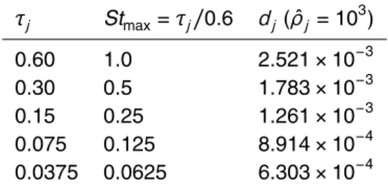
2.2 Equilibrium–Eulerian model

In the limit St_j≪1, the drag terms f_j and the thermal exchange terms Q_j can be

calculated by knowingugandTg, and the Eulerian–Eulerian model can be largely

sim-plified by considering the dusty-gas (also known as pseudo-gas) approximation (Mar-ble, 1970). A refinement of this approximation (valid ifSt_j.0.2), has been developed

5

by Maxey (1987), as a first-order approximation of the Lagrangian particle momentum balance (see Eq. 10d):

∂_tu_j+_u

j· ∇uj =

1

τ_j(ug−uj)+g. (13)

By using the Stokes law and a perturbation method (see Appendix A), and by defining

a_≡D_tug(with Dt=∂t∂ +u·∇), we obtain a correction to particle velocity up to first order

10

uj =ug+wj−τj(∂tug+uj· ∇ug)+O(τ_j2) . (14)

It can be restated

uj =ug+G− 1

j · wj−τja

+_O₍_τ2

j) (15)

G

j ≡I+τjα(∇ug)T, (16)

leading to the so-called Equilibrium–Eulerian model developed by Ferry and

Balachan-15

dar (2001), Ferry et al. (2003), and Balachandar and Eaton (2010) for incompressible

multiphase flows. Hereα is a local correction coeﬃ_{cient inserted for avoiding}

singu-larities (see Ferry et al., 2003). It is worth noting that at the zeroth order we recover

u_j =_u

g+wj, wherewj is the settling velocity defined in Eq. (5).

It is worth noting from Eq. (3) thatτ_j depends onRe_j, and it cannot be determined

20

untilu_j is known. One solution to this problem has been proposed in Ferry and

Bal-achandar (2002), whereτj is evaluated directly by knowing

f Re_j _≡

ˆ

ρjdj3|a−g|

(16)

GMDD

8, 8895–8979, 2015

volcanic plumes

M. Cerminara et al.

Title Page

Tables Figures

◭ ◮

Back Close

Full Screen / Esc

Discussion

P

a

per

|

Discussion

P

a

per

|

Discussion

P

a

per

|

Discussion

P

a

per

|

by approximating Eq. (3) in the range 0<Re_j <300. We here improved that approxi-mation in the range 0<Rej <103by using the inversion formula:

Re_j = Refj

1+_0.315_Ref0.4072

j

. (18)

Another strategy we use in the model, is to evaluate Re_j explicitly from the previous

time-step and correct it iteratively (within the PISO loop, see Sect. 3.2 below).

5

To write the compressible version of the Equilibrium–Eulerian model, we define the relativejth particle velocity fieldvj so thatuj=ug+vj. Recalling the definitions of the

mass fraction and the mixture density given above, we define:

ur=− X

j∈J

yjvj (19)

u_m=_u

g−ur (20)

10

T

r= X

j∈J

(yjvj⊗vj)−ur⊗ur, (21)

By summing up the gas momentum equation with the solid momentum equations in Eq. (10), we thus obtain:

∂t(ρmum)+∇ ·(ρmum⊗um+ρmTr)=−∇p+∇ ·T+ρmg+ X

j∈J

Sjuj. (22)

This momentum balance equation is equivalent to the compressible Navier–Stokes

15

equation with the substitutionug→um and the addition of the term ∇ ·(ρmTr) which

takes into account the first order eﬀ_{ects of particle decoupling on momentum (two-way}

coupling). We keep this term because of the presence of the settling velocitywj invj

(17)

GMDD

8, 8895–8979, 2015

volcanic plumes

M. Cerminara et al.

Title Page

Tables Figures

◭ ◮

Back Close

Full Screen / Esc

Discussion

P

a

per

|

Discussion

P

a

per

|

Discussion

P

a

per

|

Discussion

P

a

per

|

Moving to the mass conservation, summing up overi andj the continuity equations

in Eq. (10), we obtain the continuity equation for the mixture:

∂tρm+∇ ·(ρmum)= X

j∈J

Sj, (23)

while for the phases we have:

∂_t(ρmyi)+∇ ·(ρmugyi)=0 , i ∈ I (24)

5

∂_t(ρmyj)+∇ ·[ρm(ug+vj)yj]=Sj, j∈ J. (25)

It is worth noting that the mixture density follows the classical continuity equation with velocity fieldum. We refer toumas the mixture velocity field.

As pointed out in Eq. (8) and below, in our physical regime the thermal Stokes time is of the same order of magnitude of the kinematic one. However, this regime

10

has been thoroughly analyzed in the incompressible case by Ferry and Balachandar (2005), demonstrating that the error made by assuming thermal equilibrium is at least one order of magnitude smaller than that on the momentum equation (at equal Stokes number), thus justifying the limitTj →Tg=T as done for the thermal equation in the

dusty gas model.

15

By summing up all enthalpy equations in Eq. (10), and by defining hm=

P

Iyihi+ P

Jyjhj =CmT+p/ρm,Cm= P

IyiCi+ P

JyjCj andKm= P

IyiKi+ P

JyjKj, we obtain:

∂_t(ρmhm)+∇ ·[ρmhm(um+vh)]=∂tp−∂t(ρmKm)− ∇ ·[ρmKm(um+vK)]

+_{∇ ·}₍T_·_u

g−q)+ρm(g·um)+ X

j_∈J

S_j(h_j+_K

j) . (26)

The terms

20

v_h=_u_r+

P

Jyjhjvj hm

=

P

Jyj(hj−hm)vj hm

(18)

GMDD

8, 8895–8979, 2015

volcanic plumes

M. Cerminara et al.

Title Page

Tables Figures

◭ ◮

Back Close

Full Screen / Esc

Discussion

P

a

per

|

Discussion

P

a

per

|

Discussion

P

a

per

|

Discussion

P

a

per

|

vK =ur+ P

JyjKjvj Km

=

P

Jyj(Kj−Km)vj Km

, (28)

take into account the combined eﬀ_{ect of the kinematic decoupling and the di}ﬀ_erence

between the specific heat (v_h) and kinetic energy (v_K) of the mixture and of thejth specie.

Summarizing, the compressible Equilibrium–Eulerian model is:

5

∂_tρm+∇ ·(ρmum)= X

j_∈J

S_j; (29a)

∂t(ρmyi)+∇ ·(ρmugyi)=0 , i ∈ I; (29b)

∂t(ρmyj)+∇ ·(ρmujyj)=Sj, j∈ J; (29c)

10

∂t(ρmum)+∇ ·(ρmum⊗um+ρmTr)=−∇p+∇ ·T+ρmg+ X

j_∈J

Sjuj; (29d)

∂t(ρmhm)+∇ ·[ρmhm(um+vh)]=∂tp−∂t(ρmKm)− ∇ ·[ρmKm(um+vK)]

+_{∇ ·}₍T_·_u_g₋_q₎+_ρ_m₍_g_·_u_m₎+X

j_∈J

S_j(h_j+_K

j) . (29e)

15

The first equation is redundant, because it is contained in the second and third set of

continuity equations. Note that we have not used the explicit form of vj for deriving

Eq. (29), which therefore can be used for any multiphase flow model with I phases

moving with velocity u_g and temperature T, andJ phases each moving with velocity

uj =ug+vj and temperature T. However, in what follows we will use Eq. (15) when

20

referring to the compressible Equilibrium–Eulerian model.

(19)

GMDD

8, 8895–8979, 2015

volcanic plumes

M. Cerminara et al.

Title Page

Tables Figures

◭ ◮

Back Close

Full Screen / Esc

Discussion

P

a

per

|

Discussion

P

a

per

|

Discussion

P

a

per

|

Discussion

P

a

per

|

∂tψ+∇ ·(ψu) because they are the origin of the major diﬃculties in turbulence

mod-eling. A large advantage of the dusty gas and Equilibrium–Eulerian models is that in both models the the most relevant part of the drag (P_Jf_j) and heat exchange (P_JQ_j) terms have been absorbed into the conservative derivatives for the mixture. This fact allows the numerical solver to implicitly and accurately solve the particles contribution

5

on mixture momentum and energy (two-way coupling), using the same numerical tech-niques developed in Computational Fluid Dynamics for the Navier–Stokes equations. The dusty gas and Equilibrium–Eulerian models are best suited for solving multiphase system in which the particles are strongly coupled with the carrier fluid and the bulk density of the particles is not negligible with respect to that of the fluid.

10

The Equilibrium–Eulerian model thus reduces to a set of mass, momentum, and en-ergy balance equations for the gas-particle mixture plus one equation for the mass transport of the particulate phase. In this respect, it is similar to the dusty-gas equa-tions, to which it reduces forτs≡0. With respect to the dusty-gas model, here we solve

for the mixture velocityum, which is slightly diﬀerent from the carrier gas velocity ug.

15

Moreover, here kinematic decoupling is taken into account by moving theIgas phases

and theJ solid phases with diﬀ_{erent velocity fields, respectively} _u

g and uj. Thus, we

are accounting for the imperfect coupling of the particles to the gas flow, leading to

preferential concentration and settling phenomena (the vectorv_j includes a convective

and a gravity accelerations terms).

20

The Equilibrium–Eulerian method becomes even more eﬃ_{cient (relative to the}

stan-dard Eulerian) for the polydisperse case (J >1). For each species of particle tracked, the standard Eulerian method requires four scalar fields, the fast method requires one.

Furthermore, the computation of the correction tov_j needs only to be done for one

particle species. The correction has the form₋τ_ja, so once the term ais computed,

25

velocities for all species of particles may be obtained simply by scaling the correction factor based on the species’ response timesτj. To be more precise, the standard

Eule-rian method needsI+₅_J+_{4 scalar partial di}ﬀ_{erential equations, while the Equilibrium–}

(20)

GMDD

8, 8895–8979, 2015

volcanic plumes

M. Cerminara et al.

Title Page

Tables Figures

◭ ◮

Back Close

Full Screen / Esc

Discussion

P

a

per

|

Discussion

P

a

per

|

Discussion

P

a

per

|

Discussion

P

a

per

|

2.3 Sub-grid scale models

The spectrum of the density, velocity and temperature fluctuations of turbulent flows at high Reynolds number typically span over many orders of magnitude. In the cases where the turbulent spectrum extend beyond the numerical grid resolution, it is

nec-essary to model the eﬀ_{ects of the high-frequency fluctuations (those that cannot be}

5

resolved by the numerical grid) on the resolved flow. This leads to the so-called Large-Eddy Simulation (LES) techniques, in which a low-pass filter is applied to the model equations to filter out the small scales of the solution. In the incompressible case the theory is well-developed (see Berselli et al., 2005; Sagaut, 2006), but LES for com-pressible flows is still a new and open research field. In our case, we apply a spatial

10

filter, denoted by an overbar (δ is the filter scale):

ψ=

Z

Ω

G(x₋x′;δ)ψ(x′)dx′. (30)

Some example of LES filters G(x;δ) used in compressible turbulence are reviewed

in Garnier et al. (2009). In compressible turbulence it is also useful to introduce the so-called Favre filter:

15

e

ψ=ρmψ ρm

. (31)

First, we apply this filter to the Equilibrium–Eulerian model fundamental Eq. (14) modified as follows:

u_j =_u

g+wj+

−τj(∂tum+um· ∇um+(wr+uj−ug)· ∇um) (32)

20

moving the new second order terms intoO(τ_j2), using∂_ty_j+_u

j· ∇yj =0, defining: wr=−

X

j

(21)

GMDD

8, 8895–8979, 2015

volcanic plumes

M. Cerminara et al.

Title Page

Tables Figures

◭ ◮

Back Close

Full Screen / Esc

Discussion

P

a

per

|

Discussion

P

a

per

|

Discussion

P

a

per

|

Discussion

P

a

per

|

and recalling that at the leading orderuem≃ueg−wer. Multiplying the new expression for u_j byρmand Favre-filtering, at the first order we obtain:

e

uj =ueg+Ge−1· "

wj−τj eam+wer· ∇uem

− τj

ρm

∇ ·B

#

, (34)

where we have usedaem=∂tuem+uem·∇uem,eτj =τj and consequentlywej =wj because

the Stokes time changes only at the large scale and it can be considered constant at

5

the filter scale. Moreover, we have defined the subgrid-scale Reynolds stress tensor:

B=_ρ_m₍_u]

m⊗um−uem⊗uem) . (35)

As discussed and tested in Shotorban and Balachandar (2007), the subgrid terms can be consideredO(τ_j) and neglected when multiplied by first order terms.

We recall here the Boussinesq eddy viscosity hypothesis:

10

B= 2

dρmKtI−2µtSem, (36)

where the deviatoric part of the subgrid stress tensor can be modeled with an eddy viscosityµt times the rate-of-shear tensorSem=sym(∇uem)−13∇ ·uemI. The first term on

the right hand side of Eq. (36) is the isotropic part of the subgrid-scale tensor, pro-portional to the subgrid-scale kinetic energyKt. While in incompressible turbulence the

15

latter term is absorbed into the pressure, it must be modeled for compressible flows (cf. Moin et al., 1991; Yoshizawa, 1986). Ducros et al. (1995) showed another way to

treat this term by absorbing it into a newmacro-pressureand macro-temperature(cf.

also Lesieur et al., 2005; Lodato et al., 2009). We recall here also the eddy diﬀ

usiv-ity viscosusiv-ity model (cf. Moin et al., 1991): any scalar ψ transported by um generates

20

a subgrid-scale vector that can be modeled with the large eddy variables. We have:

ρm(u]mψ−eumψe)=−

µ_t

Prt∇ e

(22)

GMDD

8, 8895–8979, 2015

volcanic plumes

M. Cerminara et al.

Title Page

Tables Figures

◭ ◮

Back Close

Full Screen / Esc

Discussion

P

a

per

|

Discussion

P

a

per

|

Discussion

P

a

per

|

Discussion

P

a

per

|

wherePrt is the subgrid-scale turbulent Prandtl number.

We apply the Favre filter defined in Eqs. (31) to (29) (for the application of the Favre filter to the compressible Navier–Stokes equations cf. Garnier et al., 2009, Moin et al., 1991 and Erlebacher et al., 1990), obtaining:

∂_tρm+∇ ·(ρmuem)=Sem; (38a)

5

∂t(ρmyei)+∇ ·(ρmeugeyi)=−∇ · Yi, i ∈ I; (38b)

∂t(ρmyej)+∇ ·[ρmeujyej]=Sej− ∇ · Yj, j∈ J; (38c)

10

∂_t(ρmeum)+∇ ·(ρmuem⊗uem+ρmeTr)+∇p¯=∇ ·Te+ X

j∈J e

S_jue_j+_ρ_m_g_{− ∇ ·}B _(38d)

∂t(ρmhem)+∇ ·[ρm(eum+veh)hem]=∂tp¯−∂t(ρmKem)− ∇ ·[ρm(uem+veK)Kem]

+_{∇ ·}₍Te_·_u_e_g₋_q_e₎+_ρ_m₍_g_·_e_u_m₎+X

j_∈J e

S_j(he_j+_Ke

j)− ∇ ·(Q+QK) , (38e)

where

15

Yi =ρm(ygiug−yeieug)=−

µt

Pr_t∇yei (39a)

Yj =ρm(ygjuj−yeiuej)=− µt Prt∇

e

y_j (39b)

B=_ρ_m₍_u_m]_⊗_u_m₋_u_e_m_⊗_u_e_m₎= 2

dρmKtI−2µtSem (39c)

20

Q=_ρ_m₍_h]_m_u_m₋_he_me_u_m₎=₋µt

Prt∇ e

(23)

GMDD

8, 8895–8979, 2015

volcanic plumes

M. Cerminara et al.

Title Page

Tables Figures

◭ ◮

Back Close

Full Screen / Esc

Discussion

P

a

per

|

Discussion

P

a

per

|

Discussion

P

a

per

|

Discussion

P

a

per

|

QK =ρm(K]mum−Kemeum)=−

µt

Pr_t∇Kem, (39e)

are: the subgrid eddy diﬀ_{usivity vector of the} _i_{th phase; of the}_j_{th phase; the}

subgrid-scale stress tensor; the diﬀ_{usivity vector of the enthalpy and kinetic energy;}

respec-tively. Other approximations have been used to derive the former LES model: the viscous terms in momentum and energy equations, and the pressure-dilatation and

5

conduction terms in the energy equations are all non-linear terms and we here treat them as done by Erlebacher et al. (1990) and Moin et al. (1991). The subgrid terms corresponding to the former non-linear terms could be neglected so that, for example,

p∇ ·ug≃p∇·eug. In particular, this term has been neglected also in presence of shocks

(cf. Garnier et al., 2002). We refer to Vreman (1995) for an a priori and a posteriori

anal-10

ysis of all the neglected terms of the compressible Navier–Stokes equations. Moreover,

in our model the mixture specific heatCm and the mixture gas constantRm vary in the

domain because y_i and y_j vary. Thus, also the following approximations should be

done, coherently with the other approximations used:he_m=_C ]

mT+p/ρm≃CemeT+p/ρm

andRgmT ≃RemTe.

15

In order to close the system, terms µt,Kt and Prt must be chosen on the basis of

LES models, either static or dynamic (see Moin et al., 1991; Bardina et al., 1980; Ger-mano et al., 1991). In the present model, we implemented several sub-grid scale (SGS) models to compute the SGS viscosity, kinetic energy and Prandtl number (Cerminara,

2015b). Currently, the code oﬀ_{ers the possibility of choosing between: (1) the}

com-20

pressible Smagorinsky model, both static and dynamic (see Fureby, 1996; Yoshizawa, 1993; Pope, 2000; Chai and Mahesh, 2012; Garnier et al., 2009), (2) the sub-grid scale K-equation model, both static and dynamic (see Chacón-Rebollo and Lewandowski, 2013; Fureby, 1996; Yoshizawa, 1993; Chai and Mahesh, 2012), (3) the dynamical Smagorinsky model in the form by Moin et al. (1991), (4) the WALE model, both static

25

(24)

GMDD

8, 8895–8979, 2015

volcanic plumes

M. Cerminara et al.

Title Page

Tables Figures

◭ ◮

Back Close

Full Screen / Esc

Discussion

P

a

per

|

Discussion

P

a

per

|

Discussion

P

a

per

|

Discussion

P

a

per

|

All through this paper, we present results obtained with the dynamic WALE model (see Fig. 5 and the corresponding section for a study on the accuracy of this LES model). A detailed analysis of the influence of subgrid-scale models to simulation re-sults is beyond the scopes of this paper and will be addressed in future works.

3 Numerical solver

5

The Eulerian model described in Sect. 2, is solved numerically to obtain a time-dependent description of all intime-dependent flow fields in a three-dimensional domain with prescribed initial and boundary conditions. We have chosen to adopt an open-source approach to the code development in order to guarantee control on the nu-merical solution procedure and to share scientific knowledge. We hope that this will

10

help building a wider computational volcanology community. As a platform for devel-oping our solver, we have chosen the unstructured, finite volume (FV) method based

open source C++_{library OpenFOAM}® _{(version 2.1.1). OpenFOAM}®_{, released under}

the Gnu Public License (GPL), has gained a vast popularity during the recent years. The readily existing solvers and tutorials provide a quick start to using the code also to

15

inexperienced users. Thanks to a high level of abstraction in the programming of the source code, the existing solvers can be freely and easily modified in order to create new solvers (e.g., to solve a diﬀ_{erent set of equations) and/or to implement new}

numer-ical schemes. OpenFOAM® is well integrated with advanced tools for pre-processing

(including meshing) and post-processing (including visualization). The support of the

20

OpenCFD Ltd, of the OpenFOAM® foundation and of a wide developers and users

community guarantees ease of implementation, maintenance and extension, suited for satisfying the needs of both volcanology researchers and of potential users, e.g. in volcano observatories. Finally, all solvers can be run in parallel on distributed

mem-ory architectures, which makes OpenFOAM® suited for envisaging large-scale,

three-25

(25)

GMDD

8, 8895–8979, 2015

volcanic plumes

M. Cerminara et al.

Title Page

Tables Figures

◭ ◮

Back Close

Full Screen / Esc

Discussion

P

a

per

|

Discussion

P

a

per

|

Discussion

P

a

per

|

Discussion

P

a

per

|

The new computational model, called ASHEE (ASH Equilibrium Eulerian model) is documented in the VMSG (Volcano Modeling and Simulation Gateway) at Istituto Nazionale di Geofisica e Vulcanologia (http://vmsg.pi.ingv.it) and is made available through the VHub portal (https://vhub.org).

3.1 Finite Volume discretization strategy

5

In the FV method (Ferziger and Perić_{, 1996), the governing partial di}ﬀ_{erential equations}

are integrated over a computational cell, and the Gauss theorem is applied to convert the volume integrals into surface integrals, involving surface fluxes. Reconstruction of scalar and vector fields (which are defined in the cell centroid) on the cell interface is a key step in the FV method, controlling both the accuracy and the stability properties

10

of the numerical method.

OpenFOAM® implements a wide choice of discretization schemes. In all our test

cases, the temporal discretization is based on the second-order Crank–Nicolson

scheme (Ferziger and Perić_{, 1996), with a blending factor of 0.5 (0 meaning a}

first-order Euler scheme, 1 a second-first-order, bounded implicit scheme) and an adaptive time

15

stepping based on the maximum initial residual of the previous time step (Kay et al.,

2010), and on a threshold that depends on the Courant number (C <0.2). All

advec-tion terms of the model are treated implicitly to enforce stability. Diﬀ_{usion terms are also}

discretized implicit in time, with the exception of those representing subgrid turbulence. The pressure and gravity terms in the momentum equations and the continuity

equa-20

tions are solved explicitly. However, as discussed below, the PISO (Pressure Implicit with Splitting of Operators, Issa, 1986) solution procedure based on a pressure correc-tion algorithm makes such a coupling implicit. Similarly, the pressure adveccorrec-tion terms in

the enthalpy equation and the relative velocityv_j are made implicit when the PIMPLE

(mixed SIMPLE and PISO algorithm, Ferziger and Perić_{, 1996) procedure is adopted.}

25