438 Brazilian Journal of Physics, vol. 34, no. 2A, June, 2004
Monte Carlo Study of the Anisotropic Three-Dimensional
Heisenberg Model in a Crystal Field
R. T. S. Freire, J. A. Plascak, and B. V. da Costa
Departamento de F´ısica, ICEx, Universidade Federal de Minas Gerais
Caixa Postal 702, 30123-970 Belo Horizonte, MG, Brasil
Received on 1st December, 2003
We study the phase diagram of the three-dimensional classical ferromagnetic Heisenberg model with an easy-plane crystalline anisotropy and an easy-axis exchange anisotropy through Monte Carlo simulations. We em-ploy the Metropolis algorithm together with single-histogram techniques in order to characterize the transitions in each region of the phase diagram. Our results reveal, besides the disordered phase, the existence of Ising-like and XY-like ordered phases which are separated by a first-order transition line.
1
Introduction
Much work has been done on two- or three-dimensional Heisenberg models submitted to exchange or crystalline anisotropies [1-5]. However, as far as we know, much less work has been performed concerning the Heisenberg model submitted to both exchange and crystalline anisotropies. In this paper we focus our attention on the three-dimensional classical ferromagnetic Heisenberg model taking into ac-count the competition between these different kinds of anisotropies and determining the phase diagram of the sys-tem.
The anisotropic Heisenberg model in a crystal field can be described by the Hamiltonian
H=−J
<i,j>
Si·Sj−A
<i,j>
Sz iS
z j+D
i
(Sz i)
2 , (1)
where J,A,D are non-negative coupling constants and
< i, j >means a sum over nearest neighbor spins (in what follows we setJ = 1). The second term is related to the exchange anisotropy and behaves as an easy-axis anisotropy since it tends to align the spins in the z direction in order to lower the energy of the system. The third term, on the con-trary, corresponds to the crystalline, easy-plane anisotropy, which favors the spin alignment in the XY plane. We have, thus, a competition between the exchange anisotropy, which induces an Ising-like ordering, and the crystal field, which induces an XY-like ordering. Consequently, one expects a crossover from an Ising-like to an XY-like behavior for some special combination of A and D. In fact, it can be shown that, at zero temperature, two different phases coexist for D=3A namely, one with all the spins aligned in thez-direction and another one with all spins aligned along an arbitrary direc-tion in the x−y plane. It is the purpose of this work to study the phase diagram of this model as a function of the parameters of the Hamiltonian and locate not only the first-order transition line at finite low temperatures, but also the
second-order lines, separating these ordered phases from the disordered one, that appears at high temperatures. In the next section we present some details of the simulations and the quantities we have computed from them. The results are discussed in section 3 and the conclusions are given in the final section.
2
Simulational methods
In order to study the model above we performed Monte Carlo simulations [6, 7] and computed the specific heat
cV =L
3(< E 2
>−< E >2
)
T2 , (2)
the magnetic susceptibility
χ=L3(< m 2
>−< m >2
)
T , (3)
and itsz-component
χz=L
3(< m 2
z>−< mz>2)
T , (4)
whereE is the energy per spin, andm = 1
L3
L3
i Si and
mz =
1
L3
L3 i S
z
i are the total magnetization and its z -component, respectively. The mean value of a quantityA
is given by
< A >= 1
N−N0
N
j>N0
Aj, (5)
where N0 is the number of Monte Carlo steps per spin
R. T. S. Freire, J. A. Plascak, and B. V. da Costa 439
The global phase diagram is obtained through the lo-cation of the maxima of the specific heat and the mag-netic susceptibilities. We consider finite L×L×L lat-tices with periodic boundary conditions. To locate the max-ima we performed preliminary simulations for each value of the parameters, using a temperature step∆T = 0.1and
No= 100×L
2
Monte Carlo steps per site for the system to achieve thermal equilibrium at the lower, initial temperature. For the subsequent temperatures, we used the final configu-ration of the previous temperature as the initial configuconfigu-ration for the next one andNo= 3000MCS for reaching the new equilibrium state. Following equilibration, runs comprising up to 3×10⁴
MCS were performed in order to evaluate the corresponding thermodynamic quantities. Once we get the approximate location of the maximum from this prelim-inary simulation, we performed another one in the vicinity of the peak using∆T = 0.01with runs comprising now up to 105
MCS. This procedure has been done considering a particular lattice size, namelyL = 14. However, we have also done a finite-size scaling analysis [6-9] at some spe-cific values of the parameters by takingL = 10,12,14,16
for second-order transitions and L = 12,14,16,20,24for first-order transitions and using the single histogram re-weighting technique[10]. In this case the histograms have been taken with106
MCS for second-order and2×106
MCS for first-order transitions. From this approach we were able to obtain a more precise value for the transition tempera-tures, as well as critical exponent ratios. We have neverthe-less observed that the extrapolated transition temperatures were very close to the value obtained forL= 14(a discrep-ancy of less than 2%).
3
Results
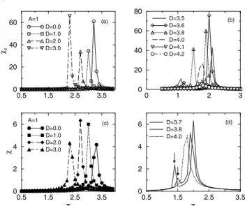
We determine the properties of the system defined by the Hamiltonian of Eq. (1) using the methods described in the previous section. We considered firstA= 1. Apart from the finite-size scaling analysis, all the curves were obtained tak-ingL= 14. To show the competition between anisotropies, Figure 1 illustrates the temperature dependence of the z -component of the magnetic susceptibility and total magnetic susceptibility for different values of the parameter D.
In both cases, we observe that the peaks initially move towards smaller temperatures with increasingD (see Figs. 1(a) and 1(c)). For D ≈ 3.5, a secondary peak appears, although more distinctively in thez-component of the mag-netic susceptibility. With further increase ofD(Figs. 1(b) and 1(d)), this secondary peak travels towards higher tem-peratures, in opposition to the primary peak, in such a way that they coalesce forD≈4.0. From this value on just one peak going to higher temperatures is observed in the mag-netic susceptibility. For the z-component of the magnetic susceptibility, this peak progressively fades away asD con-tinues to increase. A similar behavior is observed in the spe-cific heat. Associating these maxima to the phase transition we are able to plot the phase diagram for the model as in Fig. 2. This diagram reveals an Ising-like region, separated from an XY-like region by a first-order transition line. Both ordered phases are separated from the paramagnetic phase
by second-order transition lines.
0.5 1.5 2.5 3.5
T 0
2 4 6
χ
D=0.0 D=1.0 D=2.0 D=3.0
0.5 1.5 2.5 3.5
0 20 40 60
χz
D=0.0 D=1.0 D=2.0 D=3.0
0.5 1.5 2.5 3.5
T 0
2 4
6 D=3.7 D=3.8 D=4.0
0 1 2 3
0 20 40 60 80
D=3.5 D=3.6 D=3.8 D=4.0 D=4.1 D=4.2
A=1 (a)
A=1
(b)
(c) (d)
Figure 1. Behavior of the magnetic susceptibility and its z -component as a function of temperature for various values of D forA= 1andL= 14. In (d) the arrows indicate the position of the secondary peaks and the symbols have been suppressed for the sake of clarity.
0
5
10
15
D
0
1
2
3
T
Paramagnetic
XY−like
Ising−
like
Figure 2. Phase diagram for the model given by Eq. (1). Here
A= 1andL= 14. Full circles represent second-order and open circles first-order transitions. The lines are guides to the eyes and meet at a bicritical point. The error bars are of the same order as the symbol sizes and have been omitted for clarity.
In order to characterize the order of the transitions we have done a finite-size scaling analysis with the use of sin-gle histogram re-weighting techniques. Fig. 3 shows the scaling behavior of the maximum of the magnetic suscep-tibility forD = 0and D = 3 (on the Ising-like bound-ary) and D = 6 and D = 8 (on the XY-like bound-ary). One can see an expected second-order scaling behav-ior withγ/ν = 2.05(6) forD = 0 andγ/ν = 2.08(6)
forD = 3at the Ising-like boundary. As for the XY-like boundary one hasγ/ν = 2.12(6)andγ/ν = 2.13(6)for
D = 6andD = 8, respectively. Although the present ap-proach is inadequate to discriminate between the ratioγ/ν
440 Brazilian Journal of Physics, vol. 34, no. 2A, June, 2004
(namely,γ/ν = 1.970(9)and 1.97(1)[11], respectively) a clear universal second-order transition is observed for these lines at high temperatures. A finite-size scaling analysis of the critical temperature is shown in Figure 4 for several values ofD along the second-order lines. One can notice again a clear second-order scaling behavior with the extrap-olated temperatures very close to those obtained by just tak-ingL= 14. These results justify the use ofL= 14in order to obtain the phase diagram depicted in Figure 2.
2.2
2.4
2.6
2.8
ln L
1.0
1.5
2.0
2.5
ln
χ
D=0.0 D=3.0 D=6.0 D=8.0
Figure 3. Finite-size scaling analysis of the maximum of the to-tal magnetic susceptibility for particular points on the Ising-like (D = 0andD = 3) and XY-like (D = 6andD = 8) bound-aries.
0.015 0.02 0.025 0.03 0.035 L−1/ν
1.885 1.89 1.895 1.9
T
0.01 0.015 0.02 0.025 3.242
3.246 3.25 3.254 3.258
T
0.015 0.02 0.025 0.03 0.035 L−1/ν
1.95 1.96 1.97
0.01 0.015 0.02 0.025 2.32
2.33
Tc = 3.267(1)
Tc(14) = 3.259(5)
Tc = 1.876(1)
Tc(14) = 1.896(5)
Tc = 2.346(1) Tc(14) = 2.334(5)
Tc = 1.939(1) Tc(14) = 1.966(5) D=3 D=0
D=6 D=8
Figure 4. Finite-size scaling for the temperature and various values ofDalong the second-order transition lines.Tcmeans the extrapo-lated temperature andTc(14)is the corresponding value for lattice sizeL= 14. ForD= 0andD= 3we have usedνIsing= 0.630 and forD= 6andD= 8,νXY = 0.669.
0.95
1
1.05
1.1
T
−0.1
0.1
0.3
0.5
0.7
0.9
Magnetization
Figure 5. Temperature dependence of the zand xycomponents of the magnetization in the low temperature region forD = 3.5,
A = 1andL = 14. Increasing and decreasing temperatures are indicated by the arrows. The two different hysteresis curves are apparent from this figure. Open circles represent mz and open squaresmxy.
2.5 3.5 4.5 5.5 6.5
D 0.663
0.664 0.665 0.666 0.667
U4
2.3 2.5 2.7 2.9 3.1 3.3
ln L 0
1 2 3
ln
χ
slope = 3.11(4)
(a)
(b)
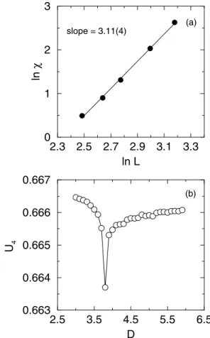
Figure 6. Characterization of the first-order transition line. (a) Finite-size scaling analysis of the maximum of the total magnetic susceptibility for a particular point on the first-order transition line namely,D = 3.8andT = 1.5. The errors are smaller than the symbol sizes. (b) Fourth-order cumulant as a function ofD for
R. T. S. Freire, J. A. Plascak, and B. V. da Costa 441
A different behavior occurs at low temperatures. Fig. 5 shows the behavior of thezandxycomponents of the mag-netization as a function of temperature for D = 3.5 and
0.95≤T ≤1.12i.e., crossing the first-order boundary. For
T ∼0.95one hasmz∼0and a finite value ofmxy, charac-terizing the XY-like phase. On the other hand, forT ∼1.1
the opposite occurs with mxy ∼ 0 and a finitemz, char-acterizing thus the Ising-like phase. The hysteresis in both magnetization curves is apparent from this figure. We have also done a finite-size scaling analysis of the maximum of the susceptibility for D = 3.8on this boundary line. The results are shown in Fig. 6(a) with a slope of3.11(4), which is reasonably close to the expected valued= 3for a first-order phase transition [9]. In addition, Fig. 6(b) also shows the fourth-order magnetization cumulant as a function ofD
forT = 1.5, which exhibits a minimum aroundD = 3.8, corresponding in fact to the transition value. From the re-sults above the first-order character of this transition line is clear.
4
Conclusions
In this work we have studied the phase diagram of the three-dimensional anisotropic Heisenberg model in a crystal field by means of Monte Carlo simulations. We have shown that the phase diagram presents, besides the disordered phase at high temperatures, an XY-like and an Ising-like phase at low temperatures. Both ordered phases undergo a second-order phase transition to the disordered phase and are separated by a first-order boundary. These lines meet at a bicritical point given byT = 1.73(3)andD= 3.95(4). A similar picture is observed for other values ofA, with the bicritical point mov-ing towards smallerT andDasAdecreases. For instance, forA= 0.5one has the bicritical point atT = 1.68(4)and
D= 2.00(3).
Acknowledgments
We would like to thank J. G. Moreira and R. Dickman for fruitful discussions, and the latter for a critical reading of the manuscript. Financial support from the Brazilian agen-cies CNPq, FAPEMIG and CIAM-02 49.0101/03-8 (CNPq) are gratefully acknowledged.
References
[1] B. V. Costa and A.S.T. Pires, J. Mag. and Mag. Mat.262(2), 316 (2003).
[2] R. van de Kamp, M. Steiner, H. Tietze-Jaensch, Physica B 241-243, 570 (1998).
[3] D. Hinzke and U. Nowak, Phys. Rev. B58(1), 265 (1998).
[4] J. Ricardo de Sousa and J. A. Plascak, Phys. Lett. A237, 66 (1997).
[5] A. Mailhot, M.L. Plumer, and A. Caill´e, Phys. Rev. B 48, 15835 (1993).
[6] M.E.J. Newman and G.T. Barkema.Monte Carlo Methods in Statistical Physics. Oxford: Clarendon, 1999.
[7] D.P. Landau and Kurt Binder.A Guide to Monte Carlo Sim-ulations in Statistical Physics. Cambridge: Cambridge Uni-versity Press, 2000.
[8] K. Binder, K. Vollmayr et al., Internat. J. Modern Phys. C 3(5), 1025 (1992).
[9] M. S. S. Challa and D. P. Landau, Phys. Rev. B34(3), 1841 (1986).
[10] A. M. Ferrenberg and R. H. Swendsen, Phys. Rev. Lett.61, 2635 (1988); A. M. FerrenbergComputer Simulation Stud-ies in Condensed Matter Physics III. Springer Proceedings in Physics,53. Heidelberg: Springer-Verlag, 1991.