Green’s functions for the wave, Helmholtz and Poisson equations
in a two-dimensional boundless domain
(Fun¸c˜oes de Green para as equa¸c˜oes da onda, Helmholtz e Poisson num dom´ınio bidimensional sem fronteiras)
Roberto Toscano Couto
1Departamento de Matem´atica Aplicada, Universidade Federal Fluminense, Niter´oi, RJ, Brasil
Recebido em 11/4/2012; Aceito em 23/6/2012; Publicado em 18/2/2013
In this work, Green’s functions for the two-dimensional wave, Helmholtz and Poisson equations are calculated in the entire plane domain by means of the two-dimensional Fourier transform. New procedures are provided for the evaluation of the improper double integrals related to the inverse Fourier transforms that furnish these Green’s functions. The integrals are calculated by using contour integration in the complex plane. The method consists basically in applying the correct prescription for circumventing the real poles of the integrand as well as in using well-known integral representations of some Bessel functions.
Keywords: Green’s function, Helmholtz equation, two dimensions.
Neste trabalho, as fun¸c˜oes de Green para as equa¸c˜oes bidimensionais da onda, Helmholtz e Poisson s˜ao cal-culadas na totalidade do dom´ınio plano por meio da transformada de Fourier bidimensional. S˜ao apresentados novos modos de se efetuarem as integrais duplas impr´oprias relacionadas `as transformadas de Fourier inversas que fornecem essas fun¸c˜oes de Green. As integrais s˜ao calculadas a partir de integrais no plano complexo. O m´etodo consiste basicamente em determinar o caminho de integra¸c˜ao que se desvia corretamente dos polos reais do integrando bem como em usar representa¸c˜oes integrais bem conhecidas de algumas fun¸c˜oes de Bessel.
Palavras-chave: fun¸c˜ao de Green, equa¸c˜ao de Helmholtz, duas dimens˜oes.
1. Introduction
Green’s functions for the wave, Helmholtz and Poisson equations in the absence of boundaries have well known expressions in one, two and three dimensions. A stan-dard method to derive them is based on the Fourier transform. Nevertheless, its derivation in two dimen-sions (the most difficult one), unlike in one and three, is hardly found in the literature, this being particularly true for the Helmholtz equation.2 This work aims at providing new ways of performing the improper dou-ble integrals related to the inverse Fourier transforms that furnish those Green’s functions in the bidimen-sional case.
It is assumed that the reader is acquainted with the usual prescriptions for circumventing the real poles of a function being integrated over the real axis: the iϵ -prescription [2–5] and that which leads to the Cauchy principal value. In this respect, Ref. [6] is closely fol-lowed. As described in this reference, in physical appli-cations, the improper integrals that arise are often not well defined mathematically, being necessary to
con-sider the physical conditions to determine the correct prescription. For this reason, the wave and Helmholtz equations solved in this work refer to concrete situa-tions.
Sections 2, 3 and 4 are devoted to the wave, Helmholtz and Poisson equations, respectively. Section 5 concludes the body of the paper with final comments.
2.
Wave equation
For the reasons given in the Introduction, in order to calculate Green’s function for the wave equation, let us consider a concrete problem, that of a vibrating, stretched, boundless membrane
∇2z(r, t)−c−2ztt=−T−1f(r, t),
[
rinR2, tinR]. (1)
In this,z(r, t) is the membrane vertical displacement at
the pointrof the xy-plane at the timet, f(r, t) is the
external vertical force per unit area, and c ≡ √T /σ,
1E-mail: [email protected].
Copyright by the Sociedade Brasileira de F´ısica. Printed in Brazil.
where T is the stretching force per unit length (uni-form and isotropic) and σ is the mass per unit area. We admit that the membrane has always been (since
t→ −∞) lying at rest on thexy-plane until the source of vibrationsf starts generating waves.
The associated Green’s functionG(r, t|r′, t′) is the
solution of (1) with a unit, point, instantaneous source at the pointr′ at the timet′
∇2G(r, t|r′, t′)−c−2Gtt=−T−1δ(r−r′)δ(t−t′)
[r
andr′inR2, tandt′ inR]. (2)
We consider here thecausal Green’s function, for which
G(r, t|r′, t′) = 0 if t < t′ , (3)
meaning that, before the instantaneous action of the unit point source, the membrane is found in its original
state - horizontally and at rest - in accordance with the causality principle.
To solve the problem defined by Eqs. (2) and (3), we Fourier transform (2), both in the spatial and time variables - according to the definitions
Fr{G(r, t|r′, t′)} ≡
1 2π
∫
R2
d2r eik·rG(r, t|r′, t′)≡G¯(k, t|r′, t′) (4)
Ft{G¯(k, t|r′, t′)} ≡
1
√
2π
∫ ∞
−∞
dt eiωtG¯(k, t|r′, t′)≡G¯˜(k, ω|r′, t′),
and solve the resulting equation to obtain ˜G¯(k, ω|r′, t′)
⌋
∇2G(r, t|r′, t′)−c−2Gtt=−T−1δ(r−r′)δ(t−t′) =Fr
⇒
−k2G¯(k, t|r′, t′)−c−2d2G/dt¯ 2= [−T−1eik·r′/(2π)]δ(t−t′) Ft =⇒
−k2G˜¯(k, ω|r′, t′) + (ω/c)2G˜¯ = [−T−1eik·r′/(2π)]eiωt′/√2π =⇒
˜¯
G(k, ω|r′, t′) = −c
2T−1eik·r′eiωt′
/(2π)3/2 ω2−k2c2 .
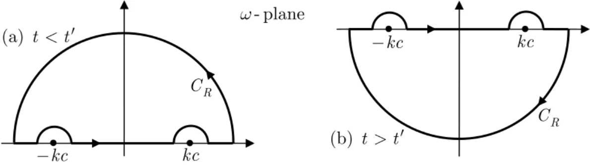
We then calculate the inverse Fourier transforms, Ft−1{G˜¯}= ¯Gfirst [carried out below, in Eq. (5)]. This is an integral of the type discussed in Ref. [6], whose evaluation as part of a contour integral in theω-plane imposes the need of prescribing the way to circumvent the two real poles atω=±kc.
For t < t′, in closing the contour with a semicircle CR of radius R → ∞, we obtain a vanishing integral
along CR if we let it lying in the upper half-plane (as
Fig. 1(a) shows), according to Jordan’s lemma. There-fore, fulfillment of Eq. (3) necessitates the path of in-tegration along the real axis to be that in Fig. 1(a),
approaching both poles from above (which is equivalent to calculate the limit asϵ→0+ of the Fourier integral
with both poles shifted of−iϵ), thus leaving both poles outside the contour and leading to the expected null result. For t > t′, we adopt this same prescription
in-dicating how the path along the real axis circumvents the poles, but, because of Jordan’s lemma, we close the contour as in Fig. 1(b), with CR in the lower
half-plane, thus enclosing both poles, at which the residues now contribute to the result.
In the notation of Ref. [6], such a way of calculating the improper integral leads to itsD−−-value3
¯
G(k, t|r′, t′) =F−1
t {G˜¯(k, ω|r′, t′)}= −
c2T−1
(2π)2 e ik·r′D
−−
∫ ∞
−∞
e−iω(t−t′)
ω2−k2c2dω= (5)
c2T−1
(2π)2 e
ik·r′·2πi·
0 (t < t′)
Res(−kc)
| {z }
eikcτ/(
−2kc)
+ Res(kc)
| {z }
e−ikcτ/(2kc)
(t > t′)
= c
2πT e
ik·r′ sinkcτ
k U(τ) ,
whereτ ≡t−t′ andU(τ) is the unit step function (equal to 0 forτ <0 and to 1 forτ >0).
3“D
−−” means that, in applying the iϵ-prescription method, both the left and right poles are shifted of−iϵ. Cauchy’s P-value as
well as theD++-,D+−- andD−+-value of the improper integral are not physically acceptable, because they do not vanish fort < t′
-
plane
kc
(a)
t
"
t
!
kc
RC
kc
kc
R
C
(b)
t
#
t
!
Figure 1 - The contours used to evaluate the integral in Eq. (5) for (a)t < t′and (b)t > t′.
Now evaluatingF−1
r of the result above, we obtain
G(r, t|r′, t′) =F−1
r {G¯(k, t|r′, t′)}= cU(τ)
(2π)2T ∫
R2
d2k e−ik·(r−r′)sinkcτ
k . (6)
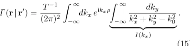
k
y
k
! "
r
r
x
k
k
Figure 2 - The axes of the Cartesian coordinateskxandkyof the vectorkused to evaluate the double integrals in Eqs. (6), (14), (19) and (25).
This double integral becomes easier to perform if we express the area element of thek-plane in the polar
co-ordinates,d2k=k dk dφ(instead of the Cartesian ones, d2k=dk
xdky), and choose thekx-axis in the opposite
direction of the vector ρ≡r−r′, as shown in Fig. 2.
In addition, noticing that k·(r−r′) =kρcos(π−φ),
we can write
G(r, t|r′, t′) = cU(τ)
(2π)2T 2π
∫
0 ∞
∫
0
eikρcosϕsinkcτ dk dφ
= cU(τ) 2πT
∞
∫
0
dksinkcτ
[ 1 2π
2π
∫
0
dφ eikρcosϕ
]
. (7)
The brackets in this equation enclose an integral repre-sentation of the Bessel function J0(kρ), which also
ad-mits another well-known integral representation; that is,4
1 2π
2π
∫
0
dφ eikρcosϕ= J0(kρ) =
2
π ∞
∫
1
du√sinkρu u2−1 . (8)
Therefore, with the substitution of this latter integral representation of J0(kρ) for the former one in Eq. (7),
we can continue the calculation as follows
G(r, t|r′, t′) =cU(τ)
2πT ∞
∫
0
dksinkcτ
[ 2
π ∞
∫
1
du√sinkρu u2−1
]
=cU(τ) 2πT
∞
∫
1 du √
u2−1 [
2
π ∞
∫
0
dksinkρusinkcτ
]
. (9)
Now recognizing that the last pair of brackets en-closes an integral representation of the delta function
δ(ρu−cτ) [8, 9] and then changing the variable of inte-gration fromutoξ=ρu−cτ, we can write
G(r, t|r′, t′) =cU(τ)
2πT ∞
∫
1
du δ(ρu−cτ)
√
u2−1 =
cU(τ) 2πT ρ
∞
∫
ρ−cτ
dξ δ(ξ) √(
ξ+cτ ρ
)2 −1
.
This integral is easily evaluated by using the sifting property of the delta function;5 we obtain
G(r, t|r′, t′) = cU(τ)
2πT ρ ×
{
0 if ρ−cτ >0 (i.e. τ−ρ/c <0) 1/
√(
cτ ρ
)2
−1 if ρ−cτ <0 (i.e. τ−ρ/c >0)
= U(τ)
2πT√τ2−(ρ/c)2 × {
0 if τ−ρ/c <0 1 if τ−ρ/c >0
| {z }
U(τ−ρ/c)
= U(τ)U(τ−ρ/c) 2πT√τ2−(ρ/c)2 .
4The first integral representation, by bisecting the range of integration and making the changing of variableφ→2π−φin the latter
part, becomes the Eq. (2) in Ref. [7],§2.3, withn= 0 andz=kρ. The second one is also found in this reference,§6.13, Eq. (3), with
ν= 0 andx=kρ.
5That is,∫b
But, in the product U(τ)U(τ−ρ/c), we can drop the first unit step function without altering the result (this is readily seen by plotting them both). We then obtain the final result
G(r, t|r′, t′) =G(ρ, τ) = 1
2πT
U(τ−ρ/c) √
τ2−(ρ/c)2 [ρ≡ |r−r
′|, τ ≡t−t′] .
3.
Helmholt equation
In this section, we calculate Green’s function for the Helmholtz equation in an unbounded two-dimensional domain. Being more specific, we solve Eq. (13), which arises in the following concrete problem.
Suppose that, in the membrane problem of the pre-vious section, the source term is given by
f(r, t) =ϕ(r)e−iω0t (t
≥t0), (10)
that is, the external vertical force per unit area varies harmonically with time with frequencyω0 at all points
of the membrane, being ϕ(r) (a non-negative function
everywhere) its maximum magnitude at the point r.
In addition, we admit that we are only interested in the stationary solution zst(r, t) that will prevail after
a very long time has elapsed as a consequence of the forced harmonic oscillation.
It is well-known that, when this steady-state motion is reached, all points of the membrane will be vibrat-ing harmonically with the same frequencyω0, but with
amplitudes described by some functionζ(r), that is
zst(r, t) =ζ(r)e−iω0t (t≫t0). (11)
Therefore, the desired stationary solution becomes de-termined as soon asζ(r) is calculated. By substituting
Eqs. (10) and (11) in Eq. (1), we verify thatζ(r) is the
solution of the two-dimensional Helmholtz equation
∇2ζ+k02ζ(r) =−T−1ϕ(r) [k0≡ω0/c], (12)
whose solution is given byζ(r) =∫
R2d2r′Γ(r|r′)ϕ(r′),
where Γ(r|r′) is the Green’s function for the above
equation, the solution of
∇2Γ +k2
0Γ(r|r′) =−T−1δ(r−r′) [randr′inR2].
(13) Since Eq. (13) is Eq. (12) withϕ(r) =δ(r−r′), we see
thatΓ(r|r′) describes the amplitude of the stationary
motion when the external vertical force is concentrated atr′ and oscillates with unit amplitude.
Let us solve Eq. (13). We first take the same Fourier transformFr defined in Eq. (4), obtaining
−k2Γ¯(k|r′) +k2
0Γ¯(k|r′) =−T−1eik·r
′
/(2π) =⇒
¯
Γ(k|r′) =T
−1
2π
eik·r′ k2−k2
0 ,
and then calculate the inverse Fourier transform
Γ(r|r′) = T
−1
(2π)2 ∫
R2
d2k e− ik·ρ k2−k2
0
[ρ≡r−r′]. (14)
We present two methods of calculating this integral in the next two subsections.
3.1. First method
To evaluate Eq. (14), we again choose the kx-axis in
the opposite direction of the vector ρ, as in Fig. 2,
but we now proceed with the Cartesian coordinates of
k=kxex+kyey
Γ(r|r′) = T
−1
(2π)2
∫ ∞
−∞
dkxeikxρ
∫ ∞
−∞
dky
k2
x+k2y−k20
| {z }
I(kx)
.
(15)
The integral denoted byI(kx) above can be
calcu-lated as part of a contour integral in the ky-plane. It
does not matter if we close the contour with a semicircle of radiusR→∞through the upper or lower half-plane; let us close it through the upper half-plane (Figs. 3 and 4). However, to investigate the poles of the integrand, we need to consider two separate cases: |kx|> k0 and |kx|< k0.
For |kx| > k0, by writing the denominator of the
integrand in the form
k2y+
(
kx2−k20 )
=(ky+ i
√
k2
x−k20 )(
ky−i
√
k2
x−k20 )
,
we verify that only the pole i√k2
x−k02 is inside the
contour (Fig. 3); therefore
-yk
plane
2 2 0
i
k
xk
2 20
i
k
xk
Im
k
yD
(a)
!2 2
0 x
k
k
Re
k
yD
(b)
!D
(c)
!!(d)
D
2 2 0 xk
k
!
!
!
!
!
!
!
!
Figure 4 - Four ways of circumventing the real poles in the evalua-tion of the integralI(kx) defined in Eq. (15) for|kx|< k0. These
are the possible iϵ-prescriptions; for each one, the corresponding
D-value (D−+, etc) is indicated.
I(kx) = 2πi Res
( i
√
k2
x−k20 )
= 2πi 1 2i√k2
x−k20
= √ π
k2
x−k20
[|kx|> k0]. (16)
For|kx|< k0, that denominator in the form k2
y−
(
k2 0−kx2
) = (
ky+
√
k2 0−kx2
)(
ky−
√
k2 0−kx2
)
clearly shows the existence of the two real poles
±√k2
0−kx2. Since the residues at them are given by
Res(±√k2 0−k2x
)
=±1/(2√k2 0−kx2
)
, we can deduce that
I(kx) =±πi
/√
k2
0−k2x [|kx|< k0] (17)
are possible values forI(kx). In fact, the + and−signs
correspond, in the notation of Ref. [6], to theD−+- and
D+−-value ofI(kx), obtained with the first and second
prescriptions shown in Fig. 4. TheD++- andD−−-value
(obtained with the third and fourth prescriptions) as well as the Cauchy P-value of I(kx) all vanish. We
proceed with both signs in Eq. (17), because only at the end, by physically analyzing the two corresponding solutions, we will be able to take the correct sign.
Let us now perform the integral with respect tokx
in Eq. (15). In view of the distinct results in Eq. (16)
and Eq. (17) forI(kx), we split the interval of
integra-tion in two (for |kx| = |k0|, convergence occurs when I(kx) = P
∫∞ −∞dky/k
2
y = 0 , which makes no
contribu-tion)
Γ(r|r′) = T
−1
(2π)2
[ ∫
|kx|>k0
dkx +
∫
|kx|<k0
dkx
]
eikxρ
I(kx)
= T−
1
(2π)2
[ ∫
|kx|>k0
dkxπ eikxρ
√
k2
x−k02 ±
∫
|kx|<k0
dkxπieikxρ
√
k2 0−kx2
]
.
The intervals of integration of both integrals above are symmetric with respect to the origin. Therefore, if we substitute coskxρ+ i sinkxρfor eikxρ, we get integrals
of odd terms (exhibiting sinkxρ), which vanish, and of
even terms (exhibiting coskxρ), which can be replaced
by twice the integral over the positive values ofkx
Γ(r|r′) =
T−1
(2π)2 [
2π∫k∞
0dkx
coskxρ
√
k2
x−k02
±2πi∫k0
0dkx
coskxρ
√
k2 0−kx2
]
.
The first integral, with the change of variable given bykx =k0u, becomes a known integral representation
of the Neumann function of order zero6
∫ ∞
k0
dkx
coskxρ
√
k2
x−k02
=
∫ ∞
1
ducos√ k0ρu u2−1 =−
π
2 N0(k0ρ). The second integral, with the change of variable kx =
k0cosϑ, also becomes a known integral representation7 ∫ k0
0 dkx
coskxρ
√
k2 0−kx2
= ∫ π/2
0
dϑcos(k0ρcosϑ) = π
2 J0(k0ρ). We thus get
Γ(r|r′) =T
−1
2π
[
−π2 N0(k0ρ)± iπ
2J0(k0ρ) ]
=
±iT−1
4 [±i N0(k0ρ) + J0(k0ρ)], which is equal to (iT−1/4) H(1)
0 (k0ρ) for the plus sign
and to (−iT−1/4) H(2)
0 (k0ρ) for the minus sign.
However, the stationary membrane motion Γ(r|r′)e−iω0t, according to the radiation condition
(see Ref. [10], p. 471), must be a wave moving away from the unit point source (i.e., from the harmonic force of unit amplitude atr′). This imposes the choice
of the first Hankel function.8 The final result is then
Γ(r|r′) =Γ(ρ) = i
4T H (1)
0 (k0ρ) [ρ≡ |r−r′|] .
(18)
6Ref. [7],§6.21, Eq. (15), where this function is denoted by Y
0 instead of N0. 7Ref. [7],§2.2, Eq. (9), withn= 0 andz=k0ρ.
8A good explanation of the representation of outgoing and incoming cylindrical waves by means of the Hankel functions is given
3.2. Second method
The integral in Eq. (14) can also be calculated in polar coordinates. The first steps are similar to those performed in going from Eq. (6) to Eq. (9)
Γ(r|r′) = T
−1
(2π)2 ∫
R2
d2k e −ik·ρ k2−k2
0
= T
−1
(2π)2 2π
∫
0 ∞
∫
0
eikρcosϕ k dk dφ k2−k2 0
=T−
1
2π ∞
∫
0 dk k k2−k2
0 [
1 2π
2π
∫
0
dφ eikρcosϕ
]
| {z }
J0(kρ)
= T−
1
2π ∞
∫
0 dk k k2−k2
0 [
2
π ∞
∫
1
du √sinkρu u2−1
]
| {z }
J0(kρ)
= T−
1 π2
∞
∫
1 du √
u2−1 [∫∞
0
dkksinkρu k2−k2
0 ]
| {z }
≡S(u)
=T−
1 π2
∞
∫
1
du S(u)
√
u2−1 . (19)
To evaluate the integralS(u) defined above, we write it in a more appropriate form
S(u) = 1 2
∞
∫
−∞ dkk
(
eikρu−e−ikρu)
2i (k2−k2 0)
= E
+(u)−E−(u)
4i
[
E±(u)≡
∫ ∞
−∞ dkk e±
ikρu
k2−k2 0
]
.
The residues of the integrands in E+(u) andE−(u) (denoted by Res+ and Res
−, respecively) at the poles±k0
are
Res+(±k0) =e±ik0ρu/2 and Res−(±k0) =e∓ik0ρu/2 .
Therefore, referring to the contours shown in Fig. 5 (which are closed with infinite semicircles that, according to Jordan’s lemma, do not contribute to the integrals), we calculate the four possibleD-values ofS(u) as follows
D−+S(u) =
[
D−+E
+(u)
− D−+E−(u)
]
/(4i) = [2πiRes+(k0)−(−2πi)Res−(−k0)]/(4i)
= (π/2)[eik0ρu/2 +eik0ρu/2]= (π/2)eik0ρu (20)
D+−S(u) =
[
D+−E+(u)− D+−E−(u)
]
/(4i) = [2πiRes+(−k0)−(−2πi)Res−(k0)]/(4i)
= (π/2)[e−ik0ρu/2 +e−ik0ρu/2]= (π/2)e−ik0ρu (21)
D++S(u) =
[
D++E
+(u) −
0
z }| {
D++E−(u)
]
/(4i) = 2πi [Res+(−k0) + Res+(k0)]/(4i)
= (π/2)[e−ik0ρu/2 +eik0ρu/2]= (π/2) cos(k
0ρu) (22)
D−−S(u) =
[ 0
z }| {
D−−E+(u)−D−−E−(u)
]
/(4i) =−(−2πi) [2πiRes−(−k0) + Res−(k0)]/(4i)
= (π/2)[eik0ρu/2 +e−ik0ρu/2]= (π/2) cos(k
0ρu) (23)
In order to determine the P-value of S(u), let us first calculate theP-values of E+(u) and E−(u) employing
the contours in Figs. 5(c) and 5(h), respectively. Denoting the semicircles of radiusr→0 used to circumvent the poles at±k0by (±k0, r) and the semicircle of radiusR→ ∞centered at the origin by (0, R), we can write
PE±(u) = lim
r→0
R→∞
[ I
C±
−
∫
(−k0,r)
−
∫
(+k0,r)
−
∫
(0,R)
✓✓✼
0]
k e±ik0ρudk
k2−k2 0
= ±2πi [Res±(−k0) + Res±(k0)]−(±πi)Res±(−k0)−(±πi)Res±(k0)− 0
=±πi [Res±(−k0) + Res±(k0)] =±πi [
e∓ik0ρu/2 +e±ik0ρu/2]=±πi cos(k
0ρu),
from which
Among the several results forS(u) calculated above, given by Eqs. (20) to (24), it is its D−+-value, given
by Eq. (20), which is to be taken and substituted in Eq. (19), because, by doing so, we obtain the correct result, that given by Eq. (18)
Γ(r|r′) = T−
1 π2
∫ ∞
1
du(π/2)eik0ρu
√
u2−1 =
i 4T H
(1) 0 (k0ρ).
Here, in the last step, we used the integral repre-sentation of the first Hankel function of order zero H(1)0 (x) = (−2i/π)
∫∞ 1 du e
iux
/√u2−1 , given in Ref. [7],
§6.13, Eq. (1).
4.
Poisson equation
To calculate Green’s function for the Poisson equation in an unbounded two-dimensional domain, that is, the solution of
∇2Ω(r|r′) = 2π δ(r−r′) [randr′inR2],
we again take the Fourier transform defined in Eq. (4), obtaining
−k2Ω(¯ k|r′) =eik·r′ =⇒ Ω(¯ k|r′) =−eik·r′/k2,
and then calculate the inverse Fourier transform:
Ω(r|r′) =− 1
2π
∫
R2
e−ik·ρ k2 d
2k [
ρ≡r−r′]. (25)
To evaluate this integral, we act as in the case of the wave equation, that is, we choose thekx-axis in the
op-posite direction of the vectorρ, as in Fig. 2, and adopt
the polar coordinateskandφofk. Next, we recognize
the integral with respect toφas the first integral rep-resentation of J0(kρ) given in Eq. (8). The result is the
following function ofρonly
Ω(r|r′) =− 1
2π 2π
∫
0 ∞
∫
0
eikρcosϕ
k2 k dk dφ=
− ∞
∫
0 dk
k
1 2π
2π
∫
0
eikρcosϕ
| {z }
J0(kρ)
=− ∞
∫
0
dkJ0(kρ)
k =Ω(ρ).
The integral with respect tokbecomes straightfor-ward if we differentiate it with respect toρ and then use the chain rule to change to a derivative with respect tok
D
E
! !
D
!E
D
!E
!D
E
!! !
D
E
!R
r
r
D
!E
D
!!E
D
E
r
r
R
0
k
0
k
0
k
0
k
(a)
(b)
(c)
(d)
-plane
k
(e)
(f)
(g)
(h)
Figure 5 - The contours in thek-plane associated to the four possibleD-values of the integralsE+(u) (at the left) andE−(u) (at the
Ω′(ρ) =−
∫ ∞
0 dk ∂
∂ρ
J0(kρ) k =
−
∫ ∞
0 dk ∂
∂k
J0(kρ) ρ =−
[J 0(kρ)
ρ
]∞
k=0
= 1
ρ ,
since J0(x) equals 1 atx= 0 and goes to 0 asx→ ∞.
Now, integrating with respect toρ, we obtain the final result
Ω(r|r′) =Ω(ρ) = lnρ+ constant [ρ≡ |r−r′|],
also obtained in Ref. [1], p. 169-170 (by a much more complicated method). The arbitrary additive constant is physically irrelevant. In fact, Green’s function for the Poisson equation can be interpreted, for instance, as the electrostatic potential atrdue to electrical charge
con-centrated at r′, and only potential differences are
rele-vant. However, unlike in the three-dimensional case, in which such constant is found to be zero by choosing the zero potential at infinite distances away from thepoint chargeatr′, this cannot be done in the two-dimensional
case, because the potential diverges (logarithmically) as the distance from theline charge atr′ increases.
5.
Final comments
As said in the Introduction, the Green’s functions con-sidered here have well known expressions, which are obtained in a number of ways (e.g., by descenting from the easier three-dimensional case). Therefore, we did not aimed at presenting new results but new meth-ods. In this respect, concerning the footnote in the first page, we should say that, for the Helmholtz equation, the procedure adopted here differs considerably from that in Ref. [1], where that equation is converted into an ordinary differential equation (in they variable) by
means of a one-dimensional Fourier transform (in thex
variable).
For the Helmholtz equation, two procedures for evaluating the inverse Fourier transform which fur-nishes the Green’s functions were presented. They differ on the coordinates used to carry on the dou-ble integrals. It seems that the calculation employing the Cartesian coordinates is somewhat less cumbersome than that based on the polar coordinates.
References
[1] B. Davies,Integral Transforms and Their Application, Texts in Applied Mathematics (Springer-Verlag, New York, 2002), 3rd ed.
[2] R. Shankar, Principles of Quantum Mechanics
(Plenum Press, New York, 1994), 2nd ed., sec. 19.4, p. 661 and p. 541.
[3] F.W. Byron Jr, and R.W. Fuller,Mathematics fo Clas-sical and Quantum Physics(Dover Publications, New York, 1992), sec. 7.4, p. 415.
[4] E. Butkov, Mathematical Physics (Addison-Wesley Publishing Company, Reading, 1973), sec. 7.7, p. 281.
[5] E. Merzbacher, Quantum Mechanics (John Wiley & Sons, New York, 1970), 2nd ed., sec. 11.3, p. 225.
[6] R. Toscano Couto, Revista Brasileira de Ensino de F´ısica29, 3 (2007).
[7] G.N. Watson,A Treatise on the Theory of Bessel Func-tions(Cambridge University Press, London, 1944), 2nd ed.
[8] G.B. Arfken and H.J. Weber, Mathematical Methods for Physicists (Harcourt Academic Press, San Diego, 2001), 5th ed., Prob. 1.15.24.
[9] R. Toscano Couto, TEMA Tend. Mat. Apl. Comput.
11, 57 (2010).
[10] F.B. Hildebrand, Advanced Calculus for Applications