Extension of application field of analytical formulas for the computation
of projectile motion in midair
(Extens˜ao do campo de aplica¸c˜oes de f´ormulas anal´ıticas para os c´alculos do movimento de um proj´etil no ar)
Peter Chudinov
1Perm State Agricultural Academy, Perm, Russian Federation
Recebido em 12/4/2012; Aceito em 23/6/2012; Publicado em 18/2/2013
The classic problem of the motion of a point mass (projectile) thrown at an angle to the horizon is reviewed. The air drag force is taken into account with the drag factor assumed to be constant. An analytical approach is used for the investigation. Application field of the previously obtained approximate analytical formulas has been expanded both in the upward launch angle , and in the direction of increase of the initial speed of the projectile. The motion of a baseball is presented as an example. It is shown that in a sufficiently wide ranges of initial velocity and launch angle the relative error in calculating the distance of the ball does not exceed 1%.
Keywords: spherical object, quadratic drag force, analytical formula, relative error.
O problema cl´assico do movimento de um ponto material (proj´etil) jogado com determinado ˆangulo em rela¸c˜ao `a dire¸c˜ao horizontal ´e revisto nesse artigo. A for¸ca de resistˆencia do ar ´e levada em conta, supondo que o coeficiente de arrastamento seja constante. Uma abordagem anal´ıtica ´e utilizada para essa investiga¸c˜ao. O campo de aplica¸c˜ao das f´ormulas anal´ıticas aproximadas obtidas anteriormente foi expandido tanto em rela¸c˜ao ao ˆ
angulo de lan¸camento quanto em rela¸c˜ao aos valores da velocidade inicial do proj´etil. O movimento de uma bola de basebol ´e apresentado como exemplo. Mostra-se que, para intervalos suficientemente amplos de velocidade inicial e ˆangulo de lan¸camento, o erro no c´alculo da distˆancia percorrida pela bola n˜ao ´e superior a 1%.
Palavras-chave: objeto esf´erico, for¸ca quadr´atica de arrastamento, f´ormulas anal´ıticas, erro relativo.
1. Introduction
The problem of the motion of a point mass (projec-tile) thrown at an angle to the horizon has a long his-tory. The number of works devoted to this task is im-mense. It is a constituent of many introductory courses of physics. This task arouses interest of authors as be-fore [1-6]. With zero air drag force, the analytic solu-tion is well known. The trajectory of the projectile is a parabola. In situations of practical interest, such as throwing a ball, taking into account the impact of the medium the quadratic resistance law is usually used. In that case the problem probably does not have an exact analytic solution and therefore in most scientific publications it is solved numerically [7-11]. Analytic approaches to the solution of the problem are not suf-ficiently advanced. Meanwhile, analytical solutions are very convenient for a straightforward adaptation to ap-plied problems and are especially useful for a qualitative analysis. Therefore the attempts are being continued to construct analytical solutions (even approximate) for this problem. Comparativly simple approximate
ana-lytical formulas to study the motion of the point mass in a medium with a quadratic drag force have been ob-tained using such an approach [12-14]. These formulas make it possible to carry out a complete qualitative and quantitative analysis without using numerical integra-tion of differential equaintegra-tions of point mass mointegra-tion. The proposed analytical solution differs from other solutions by easy formulas, ease of use and acceptable accuracy. It is intended to study the motion of a baseball, and other similar objects.
Present article is largely initiated by the interest-ing work of Hackborn [4]. In this paper the accuracy of various analytical approximations of the projectile trajectories was investigated in the calculation of their distance in a fairly wide ranges of variation of the ini-tial velocity and launch angle. The purpose of present paper is to extend the application field of the formu-las [12-14] and to compare the accuracy of these for-mulas for calculating the projectile range with the re-sults obtained in Ref. [4]. In the paper under con-sideration the term “point mass” means the center of mass of a smooth spherical object of finite radiusrand
1
E-mail: [email protected].
cross-sectional area S = πr2. The conditions of
ap-plicability of the quadratic resistance law are deemed to be fulfilled, i.e. Reynolds number Re lies within 1×10³< Re <3×10⁵ [5].
2.
Equations of point mass motion and
analytical formulas for basic
param-eters
Suppose that the force of gravity affects the point mass together with the force of air resistance R (Fig. 1), which is proportional to the square of the velocity of the point and directed opposite the velocity vector. For the convenience of further calculations, the drag force will be written as R = mgkV2. Here m is the mass
of the projectile, g is the acceleration due to gravity,
k is the proportionality factor. Vector equation of the motion of the point mass has the form
mw=mg+R,
where w - acceleration vector of the point mass. Dif-ferential equations of the motion, a commonly used in ballistics, are as follows [15]
dV
dt =−gsinθ−gkV 2, dθ
dt =− gcosθ
V , dx
dt =Vcosθ, dy
dt =Vsinθ. (1)
HereV is the velocity of the point mass,θ is the angle between the tangent to the trajectory of the point mass and the horizontal, x,y are the Cartesian coordinates of the point mass,k= ρacdS
2mg =constis the
proportion-ality factor,ρa is the air density,cd is the drag factor
for a sphere, and S is the cross-section area of the ob-ject (Fig. 1). The first two equations of the system (1) represent the projections of the vector equation of mo-tion for the tangent and principal normal to the trajec-tory, the other two are kinematic relations connecting the projections of the velocity vector point mass on the axisx,y with derivatives of the coordinates.
The well-known solution [15] of Eqs. (1) consists of an explicit analytical dependence of the velocity on the slope angle of the trajectory and three quadratures
V(θ) = V0cosθ0 cosθ√1 +kV2
0cos2θ0(f(θ0)−f(θ)) ,
f(θ) = sinθ cos2θ + ln
( tan
(
θ
2 +
π
4 ))
, (2)
t=t0−1
g θ
∫
θ0 V
cosθdθ, x=x0−
1
g θ
∫
θ0
V2dθ, (3)
y=y0−1
g θ
∫
θ0
V2tanθdθ.
Figure 1 - Basic motion parameters.
HereV0andθ0 are the initial values of the velocity and the slope of the trajectory respectively, t0 is the initial value of the time, x0, y0 are the initial values of the coordinates of the point mass (usually accepted
t0=x0 =y0 = 0). The derivation of the formulas (2) is shown in the well-known monograph [16].
The integrals on the right-hand sides of Eqs. (3) cannot be expressed in terms of elementary functions. Hence, to determine the variables t, x and y we must either integrate Eqs. (1) numerically or evaluate the definite integrals (3). To avoid these procedures, com-paratively simple approximate analytical formulas for the eight basic parameters of point mass motion were obtained in [12-14] (Fig. 1). The four parameters corre-spond to the top of the trajectory, four - to the point of drop. We will give a complete summary of the formulas for the maximum height of ascent of the point massH, motion timeT, the velocity at the trajectory apexVa,
flight rangeL, the time of ascentta, the abscissa of the
trajectory apex xa, impact angle with respect to the
horizontalθ1 and the final velocityV1
H = V
2 0sin2θ0 g(2 +kV2
0sinθ0)
, T = 2 √
2H g ,
Va=
V0cosθ0
√
1 +kV2
0(sinθ0+ cos2θ0lntan(θ02 + π 4)) L=VaT, ta =
T−kHVa
2 , xa=
√
LHcotθ0,
θ1=−arctan
[ LH
(L−xa)2
]
, V1=V(θ1). (4)
mass, respectively. Formulas (4) enable us to calcu-late the basic parameters of motion of a point mass directly from the initial data V0, θ0, as in the theory of parabolic motion. With zero drag (k=0), formulas (4) go over into the respective formulas of point mass parabolic motion theory.
As an example of the use of formulas (4) we calcu-lated the motion of a baseball with the following initial conditions
V0 = 45 m/s;θ0 = 40◦;
k= 0.000548 s2/m2, g = 9.81 m/s2.
The results of calculations are recorded in Table 1. The second column shows the values of parameters ob-tained by numerical integration of the motion Eqs. (1) with the fourth-order Runge-Kutta method. The third column contains the values calculated by formulas (4). The deviations from the exact values of parameters are shown in the fourth column of the table.
Table 1 - Numerical and analytical values of parameters.
Parameter Numerical value Analytical value Error (%)
H, m 30.97 31.43 +1.5
T, s 5.00 5.06 +1.2
Va, m/s 23.19 23.19 0.0
L, m 117.8 117.4 -0.3
ta, s 2.35 2.33 -0.9
xa, m 65.36 66.32 +1.5
θ1, deg -53.04 -54.73 +3.2
V1, m/s 27.45 27.99 +2.0
3.
Extension of application field of the
formulas (4)
For baseball typical values of the drag force coefficient
kis about 0.0005/0.0006 s2/m2[4, 9]. We introduce the
notationp=kV2
0. The dimensionless parameterphas
the following physical meaning - it is the ratio of air re-sistance to the weight of the projectile at the beginning of the movement. Formulas (4) have a bounded region of application. The main characteristics of the motion
H,T,Va,L,ta,xa,θ1,V1have accurate to within 2-3%
for values of the launch angle, initial velocity and the parameter pfrom ranges
0◦≤θ0≤ 70◦, 0≤V0≤50 m / s, 0≤ p ≤1.5. (5)
We transform the formulas (4) so as to improve the accuracy of calculating the basic measure of the motion - range L in the entire range of launch angles and at values of the initial velocity and the parameterplarger than compared with the ranges of Eq. (5)
0◦≤θ0≤ 90◦, 0≤V0≤80 m/s, 0 ≤p≤4. (6)
For this we consider the structure of the range for-mula L = VaT. According to this formula, range of
the motion is defined as the product of the velocity at the top of the trajectory Va on the time motion T
Therefore, to increase the accuracy of computation of the rangeL it is necessary to increase the accuracy of calculating the parametersVa and T. Let’s start with
the increase the accuracy of the parameterT. In turn, according to the second of the formulas (4), the time of the projectile motionT is determined by parameter
H. The formula for the maximum height of ascent of the projectileH is the most important of all the formu-las (4). When the launch angleθ0 increases, height H
computed according to the first formula (4) is behind the exact value of this parameter. The exact value ofH
can be obtained by integrating the equations of motion (1). The greatest noncoincidence occurs at an angle of throwingθ0= 90◦. It is known [15] that the maximum
height attained by the point mass at throwing with the initial conditionsV0,θ0= 90◦, is given by
Hmax= 1
2gk ln(1 +kV 2
0). (7)
Formula (4) forH at θ0= 90◦ gives the value of
H1= V
2 0 g(2 +kV2
0)
. (8)
We introduce the notation
∆h=Hmax−H1=
1
2gkln(1 +kV 2 0)− V2
0 g(2 +kV2
0) .
The quantity ∆h- is a mismatch between the exact and approximate values of the height atθ0 = 90◦. We
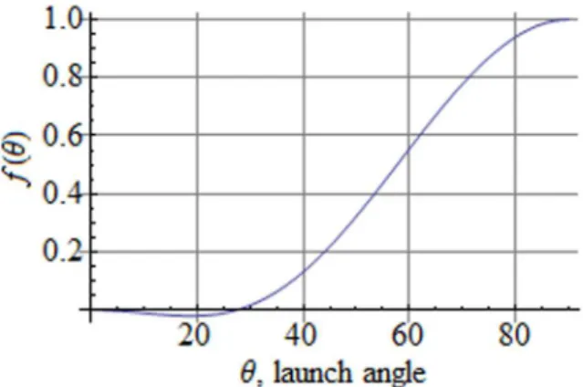
form the functionf(p), equal to the ratio (8) to (7)
f(p) = H1
Hmax
= 2p
(2 +p)ln(1 +p). (9)
The graph off(p) is shown in Fig. 2.
The graph shows that when the force of air resis-tance increases (parameterpgrows), formula (4) forH
loses accuracy whenθ0= 90◦. The same holds for large
angles of throwing θ0 ≥70◦. To eliminate this
draw-back, we modify the formula (4) for H. Let it be like this
H = V
2 0sin2θ0 g(2 +kV2
0sinθ0)
+ ∆h·f1(θ0). (10)
Heref1(θ0) is a function of the launch angle satisfying
f1(0◦) = 0, f1(90◦) = 1. The choice of this function is
quite arbitrary. Let the functionf1(θ0) be given by the following empirical formula
f1(θ0) = sin4θ0− (θ0
90 )2
·cos6θ0.
Graph of this function is shown in Fig. 3. Such a structure of formula (10) allows more accurate calcula-tion of the heightH at high angles of throwingθ≥70◦.
Whenθ0 = 90◦, formula (10) gives the exact value of
the height (7).
Figure 3 - Graph of the functionf1=f1(θ0).
Now we transform the second factorVa in the range
formula. The parameter Va is the velocity of the
pro-jectile at the top of the trajectory calculated by the formulas (2) at θ = 0◦. Instead of the values of the
velocity at the top of the trajectory atθ = 0◦ we
cal-culate the velocity of the projectile at some close point of the trajectory defined by the angle of inclinationθa.
We define angleθa, measured in degrees, as a function
of the parameters pandθ0: θa =f2(p, θ0). The choice
of this function is arbitrary. However, the value of θa
should be positive in order to increase the velocity of the projectile compared with the value of it at the top of the trajectory. This follows from the well-known fact that on the upward trajectory velocity is greater than at the top. We define the functionf2 as follows
θa=f2(p, θ0) =p· π
180·
θ0
90 ·(1 + 2·sin2θ0). (11)
Now underVa we understand the value determined
by the relation
Va=V(θa). (12)
Thus, the formulas (4) for H and Va are replaced
by the formulas (10), (12). In the absence of resis-tance of the medium (k = 0) formulas (10), (12) turn into the corresponding formulas of the parabolic motion theory. In addition, formulas (4) make it possible to ob-tain simple approximate analitical expressions for the basic functional relationships of the problemy(x),y(t),
y(θ), x(t),x(θ), t(θ) [13]. For example, the trajectory equationy(x) has the form
y(x) = Hx(L−x)
x2
a+ (L−2xa)x
. (13)
This formula shows that for the construction of de-pendence y(x) we need to know three parameters: H,
Land xa, which are determined by formulas (4). This
dependencey(x) provides a shift of apex of the path to the right and has a vertical asymptote, as it is in case of the of projectile trajectories in the air. In the absence of the resistance L= 2xa and formula (13) go into the
corresponding formula of the theory of parabolic mo-tion.
4.
The results of calculations and their
comparison
The formulas (10), (12), (13) were used to calculate the motion of a baseball. It is convenient to calcu-late the coefficient of resistance k in these formulas by means of the terminal velocity of a ball (Fig. 1):
k= 1/V2
term. We used the following typical values ofk
(forVterm= 40 m/s) and the acceleration of gravityg
k= 1
402 = 0.000625 s
2/m2, g= 9.81 m/s2
. (14)
The initial velocity, launch angle and parameter p
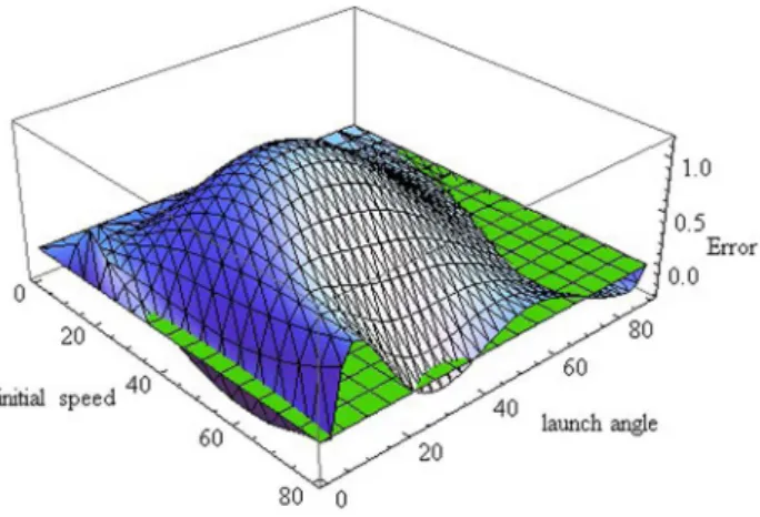
Figure 4 - The relative error in calculating the distance (in %).
The horizontal plane in Fig 4 corresponds to the zero value of the relative error. Figure 4 shows that in the covered scope (6) the relative error is less than 1%. Figure 5 shows the projectile trajectoryy(x) for values ofV0= 80 m/s,θ0= 60◦. The solid line is obtained by
integrating Eqs. (1), the broken line is constructed by formulas (4), (10), (12), (13). It is obvious that these formulas approximate a precise trajectory quite well. In paper [4] well-known analytical approximations of the trajectory of Parker [7], Littlewood [17], Lamb [18] are quoted, and also Hackborn gave his original formula, close to above-mentioned ones. These approximations were used in [4] to calculate the distance of baseball motion in the ranges of initial velocity and launch an-gle 10 ≤ V0 ≤ 80 m/s, 15◦ ≤ θ0 ≤ 75◦ for values of
Eq. (14). The relative error in calculating the distance for these approximations was calculated in Ref. [4]. It was found by Hackborn that in these ranges the rela-tive error reaches 4.5%÷6.5%. These values are much higher than the accuracy of 1% obtained with the help of formulas (4), (10), (12), (13).
Figure 5 - Graph of the functiony=y(x).
5.
Conclusions
The proposed modification of the formulas [12-14] al-lows us to significantly expand the range of their use in the studying of the projectile motion in midair. All the basic parameters of the motion and functional depen-dencies are still described by simple analytical relations. In addition the numerical values of the required quan-tities are determined with high accuracy. Thus, the formulas (4), (10), (12), (13) make it possible to study the motion of a point mass in a medium with resistance in the way it is done for the case of no drag.
References
[1] G.F.L. Ferreira, Revista Brasileira de Ensino de F´ısica
23, 271 (2001).
[2] A.D.S. Bruno and J.M.O. Matos, Revista Brasileira de Ensino de F´ısica24, 30 (2002).
[3] E.N. Miranda, S. Nikolskaya and R. Riba, Revista Brasileira de Ensino de F´ısica26, 125 (2004).
[4] W. Hackborn, Canadian Applied Mathematics Quar-terly14, 285, (2006)
[5] A.Vial, European Journal of Physics28, 657 (2007).
[6] J. Benacka, International Journal of Mathematical Ed-ucation in Science and Technology41, 373 (2010).
[7] G. Parker, American Journal of Physics45, 606 (1977).
[8] H. Erlichson, American Journal of Physics 51, 357 (1983).
[9] A. Tan, C. Frick and O. Castillo, American Journal of Physics55, 37 (1987).
[10] C. Groetsch, American Journal of Physics 65, 797 (1997).
[11] J. Lindemuth, American Journal of Physics 39, 757 (1971).
[12] P. Chudinov, International Journal of Mathematical Education in Science and Technology41, 92 (2010).
[13] P. Chudinov, International Journal of Sports Science and Engineering5, 27 (2011).
[14] P. Chudinov, European Journal of Physics 25, 73 (2004).
[15] B. Okunev,Ballistics (Voyenizdat, Moscow, 1943). [16] S. Timoshenko and D. Young, Advanced Dynamics
(McGraw-Hill Book Company, New York, 1948).
[17] J. Littlewood, Mathematical Spectrum4, 80, (1971).