Forças de depleção exercidas por matéria ativa e passiva em colóides passivos

(1)

UNIVERSIDADE FEDERAL DO CEARÁ CENTRO DE CIÊNCIAS

DEPARTAMENTO DE FÍSICA

PROGRAMA DE PÓS-GRADUAÇÃO EM FÍSICA

Levi Rodrigues Leite

Forças de depleção exercidas por matéria ativa e passiva em

colóides passivos

Depletion forces exerted by active and passive matter on

passive colloids

(2)

Levi Rodrigues Leite

Forças de depleção exercidas por matéria ativa e passiva em

colóides passivos

Depletion forces exerted by active and passive matter on

passive colloids

Tese apresentada ao Curso de Pós-graduação em Física da Universidade Federal do Ceará como parte dos requisitos necessários para a obtenção do título de Doutor em Física.

Orientador:

Prof. Dr. Wandemberg Paiva Ferreira

DOUTORADO EM FÍSICA DEPARTAMENTO DE FÍSICA

PROGRAMA DE PÓS-GRADUAÇÃO EM FÍSICA CENTRO DE CIÊNCIAS

UNIVERSIDADE FEDERAL DO CEARÁ

Fortaleza - CE

(3)

Dados Internacionais de Catalogação na Publicação Universidade Federal do Ceará

Biblioteca Universitária

Gerada automaticamente pelo módulo Catalog, mediante os dados fornecidos pelo(a) autor(a)

L554f Leite, Levi Rodrigues.

Forças de depleção exercidas por matéria ativa e passiva em colóides passivos / Levi Rodrigues Leite. – 2017.

133 f. : il. color.

Tese (doutorado) – Universidade Federal do Ceará, Centro de Ciências, Programa de Pós-Graduação em Física , Fortaleza, 2017.

Orientação: Prof. Dr. Wandemberg Paiva Ferreira.

1. Colóides . 2. Matéria ativa. 3. Força de depleção . I. Título.

(4)

L

EVI RODRIGUES LEITE

Forças de depleção exercidas por matéria ativa e passiva em colóides

passivos

Depletion forces exerted by passive and active matter on passive colloids

Tese de doutorado apresentada ao Curso de Pós-graduação em Física da Universidade Federal do Ceará como parte dos requisitos necessários para a obtenção do título de Doutor em Física.

Aprovada em: 30/03/2017.

BANCA EXAMINADORA

Prof. Dr. Wandemberg Paiva Ferreira (Orientador) Departamento de Física – UFC

Prof. Dr. Fabrício Queiroz Potiguar

Instituto de Ciências Exatas e da Natureza – UFPA

Dr. Diego de Lucena Camarão Departamento de Física – UFC

Prof. Dr. Aristeu Rosendo Pontes Lima

Instituto de Ciências Exatas e da Natureza – UNILAB

(5)

(6)

Acknowledgments

I would like to thank my advisor Prof. Dr. Wandemberg Paiva Ferreira, for trust in me as his student and for the support all these years, always being present when necessary and sharing his teachings.

I would like to thank Prof. Fabrício Queiroz Potiguar for all his support on the development of the works presented in this thesis, as well as the suggestions for personal improvements.

I also thank the other members of the jury: Dr. Diego de Lucena Camarão, Prof. Aristeu Rosendo and Prof. Gil de Aquino for all the help and suggestions gave on this thesis and for my personal career.

I would like to thank very much all my friends that were together with me in this journey: Cesar Vieira, Daniel Gomes, Daniel Marchesi, Davi Dantas, Diego Lucena,

Diego Ximenes,Heitor Credidio, Hygor Piaget,Leandro Jader, Rafael Alencar, Rilder de Sousa, Saulo Dantas, Vagner Bessa, (...). To my colleagues of the GTMC group: André Borba, Danilo Borges, David Figueiredo, Diego Frota, Felipe Munarin, Florêncio Batista,

Jessé Pereira, João Cláudio and Jorge Capuan.

A special thanks of course goes to my parentsPedro Fausto Rodrigues Leite and Rosa Helena Rodrigues Leite, as well as my brother Pedro Fausto Rodrigues Leite Júnior, for all the support in my career as a physicist. I also thank my wifeTabata Vieira de Araujo

for understand and support my efforts as a doctorate student.

I would like to thank all professors of the physics department at UFC, specially Prof. Dr. Valder Nogueira Freire, who accepted me as his graduate student and Prof. Dr. Gil de Aquino Farias, who gave me the support for finding a research area for my master and doctor degrees.

I would like to thank the Brazilian agencies CNPq, CAPES and FUNCAP for all the financial support received along seven years.

(7)

“Let come what comes, let go what goes. See what remains.”

(8)

Resumo

Nesta tese propõe-se o estudo da influência das forças de depleção induzidas em partículas passivas em função do meio (partículas) que as circundam.

Na primeira parte do trabalho, estudam-se as forças de depleção exercidas por partícu-las ativas (auto-propelidas) em objetos passivos circulares e elípticos através do cálculo numérico. Mostra-se que um banho de partículas ativas pode induzir forças repulsivas e atrativas que são sensíveis à forma e orientação dos objetos passivos. Em geral, a força resultante nos objetos passivos devido às partículas ativas são estudadas como função da forma e orientação dos objetos passivos, magnitude do ruído angular e distância entre os objetos passivos. No caso em que a separação entre objetos passivos é menor que um diâmetro de partícula ativa, o aumento desta separação resulta em um aumento da magnitude das forças de depleção, que são repulsivas neste caso. Para distâncias entre os objetos passivos maiores que um diâmentro da partícula ativa, a magnitude da força de depleção sempre decresce com o aumento da distância entre as partículas passivas. Observa-se também que a natureza da força de depleção (atrativa ou repulsiva) depende da forma e orientação relativa das partículas passivas. Observa-se que uma força de de-pleção atrativa ocorre quando objetos passivos de forma elíptica são dispostos lado a lado, mas de modo que os semi-eixos maiores estão paralelos e não alinhados. Isto ocorre para uma densidade suficientemente alta do banho de partículas ativas.

(9)

Abstract

In this thesis it is proposed a study of the influence of the depletion forces induced by passive particles as a function of the medium (particles) that surrounds then.

In the first part of this thesis, the depletion forces exerted by active (self-propelled) particles on passive and elliptical passive objects are studied through numerical simula-tions. It is shown that a bath of active particles can induce repulsive and attractive forces that are sensitive to the shape and orientation of the passive objects. In general, the force resulting in passive objects due to the active particles is studied as a function of the shape and orientation of the passive objects, magnitude of the angular noise, and distance between passive objects. In the case where the separation between passive objects is less than an active particle diameter, the increase of this separation results in an increase of the magnitude of the depletion forces, which are repulsive in this case. For distances be-tween passive objects larger than one diameter of the active particle, the magnitude of the depletion force always decreases with increasing distance between the passive particles. It is also observed that the nature of the depletion force (attractive or repulsive) depends on the shape and relative orientation of the passive particles. It is noted that an attractive depletion force occurs when elliptical passive objects are arranged side by side, but so that the semi-major axis are parallel and not aligned. This occurs for a sufficiently high concentration (or density) of active particles.

(10)

List of Figures

1.1 Illustration of the potential energy curve as a function of the interatomic distance. The total interaction is a combination of a short-range repulsion and a long-range attraction. . . 35

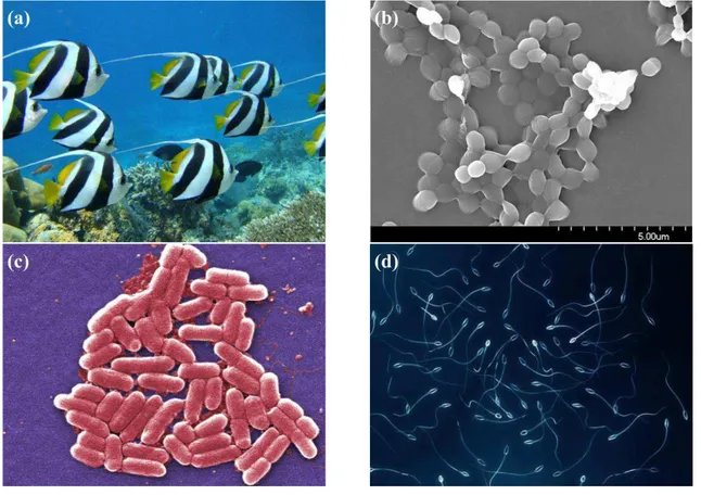
1.2 Examples of active matter systems which form agglomerate and present collective behaviour: (a) fishes; (b) bacterial colony; (c) Escherichia coli

and (d) Spermatozoa. . . 38

1.3 An example of microscopic artificial swimmer. (a) A chain of paramagnetic beads linked by DNA can be used as a propeller. (b) Experimental motion sequence of such a propeller pulling a red blood cell. Image extracted from ref. [75]. . . 39

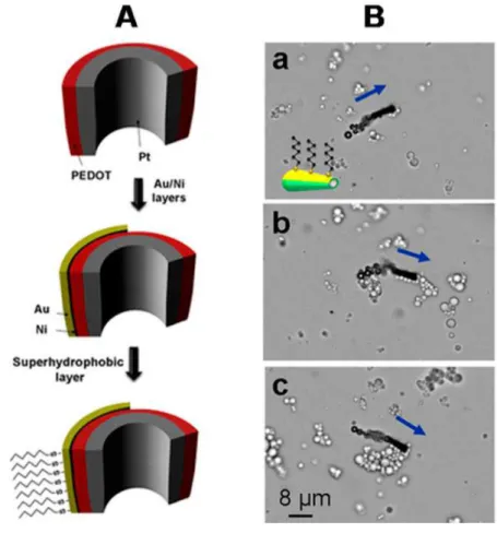
1.4 An example of a self-propelled micromachine for the removal of oil droplets. (a) Cross-section of a superhydrophobic SAM-modified Au/Ni/PEDOT/Pt tubular microengine. (b) Hexanethiol-modified microsubmarine transport-ing a payload of multiple oil droplets. Image extracted from ref.[120]. . . . 42

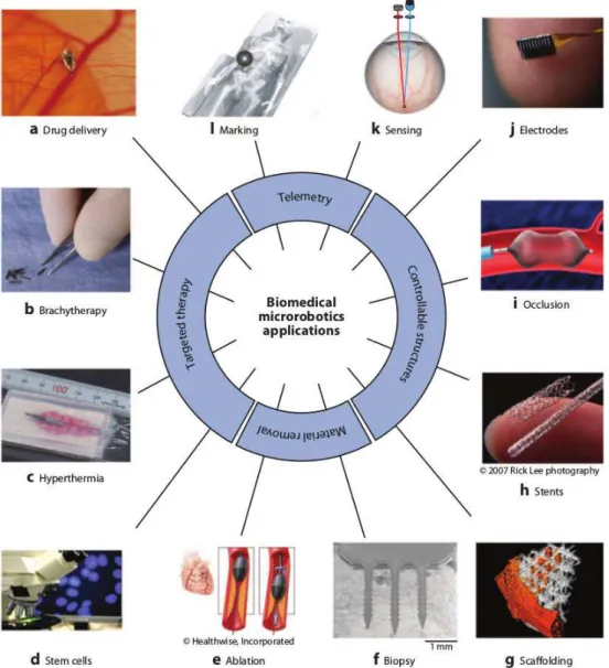
1.5 Biomedical microrobots applications, relating with its fundamentals branches: telemetry, targeted therapy, controllable structures and material removal. Image extracted from ref.[75]. . . 44

1.6 Illustrative scheme for particle-wall interaction. (a) Checks if particles is inside the obstacle; (b) the boundary of the obstacle is approximated by its tangent l at the point p where the particle entered the obstacle and (c) particle change its position according to the reflecting line. Picture extracted from reference [151]. . . 45

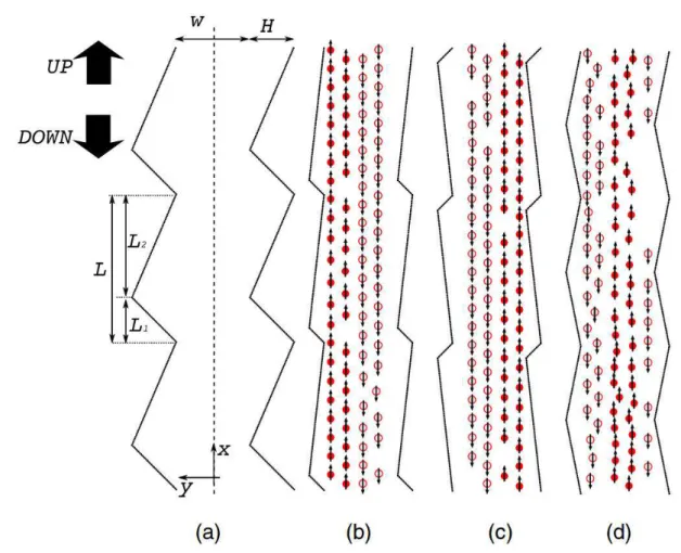
1.7 Snapshots showing wedges capturance in function of the inner angle φ. Picture extracted from reference [170]. . . 46

1.8 Different rectification patterns of pedestrian flows for (a) a channel of depth

(13)

xii

1.9 Cluster formation induced by immovable red disks. (a-d) As time evolves, particles goes from an initial fluctuating state to a dynamically frozen steady state around the obstacles. Picture extracted from reference [187]. . 48

1.10 Illustration of two different forms of colloidal stabilization. On the top, stabilization is performed by electrostatic contributions induced by added ions; on the bottom, colloidal stabilization by steric contributions induced by added polymers, causing repulsion due to the unfavorable decrease in entropy. . . 49

1.11 Interaction energy curve W(h)/kBT versus h/σ separation between

sus-pended large spheres, where the attraction and repulsion are evident. Im-age extracted from reference [191].. . . 50

1.12 Entropic force profile between a pair of hard macrospheres in a fluid com-posed of microspheres with a diameter five times smaller. Image extracted from reference [192]. . . 51

1.13 (a) Sketch explaining how repulsion arises on spherical particles induced by self-propelled particles (b) Typical snapshot for the two colloidal disks in an active bath. Image extracted from reference [199]. . . 52

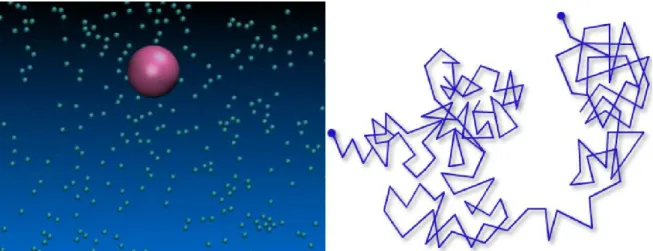
2.1 Illustration of brownian motion. Small particles collide with big particles inducing an random trajectory. . . 55

2.2 Illustration of the run-and-tumble motion, exerted by bacteria such as E. Coli. Picture extracted from reference [227]. . . 59

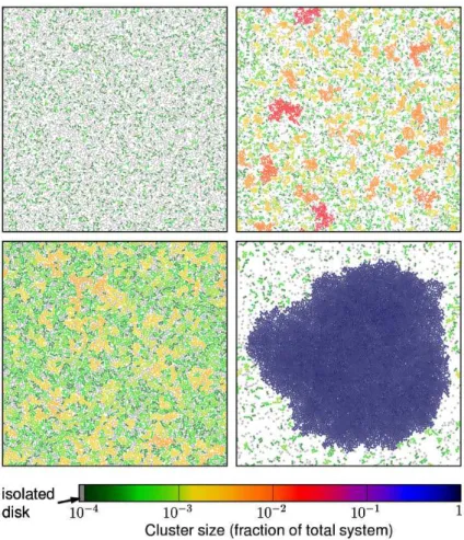
2.3 Snapshots of104 _{disks, showing different clusters size for different densities}

and self-propulsion velocities. Image extracted from reference [54]. . . 60

2.4 (a-d) Examples of pattern formation for different densities and noise values, for constant self-propulsion velocity. Image extracted from reference [21]. . 61

2.5 Illustration of a two-dimensional cross section of the overlapping volume between hard spheres. RS is the smaller particle diameter, RB is the big

particle diameter and l is the width of a lens formed by spherical caps. . . 63

2.6 The force between two spherical bodies in a solution of spherical macro-molecules. Figure extracted from reference [228]. . . 64

2.7 Two fixed hard spheres of radius Rb. denoted as 1 and 2, in a fluid of

smaller hard spheres of radius Rs. Picture extracted from reference [193]. . 65

2.8 Illustration of the Derjaguin model for two spherical particles relating it to two flat surfaces distant apart by z. Extracted from reference [229] . . . . 67

(14)

xiii

2.10 At high densities small particles forms layers around big particles. If the gap between the plates is commensurate to the diameter of small sphere, the free energy is smaller than at separations incommensurate with the small sphere diameter. This causes the depletion force to oscillate. Image

extracted from reference [232]. . . 68

2.11 A scheme of laser radiation experiment, where the depletion attraction between a colloidal sphere and a plate was measured. Image extracted from reference [233]. . . 70

2.12 A scheme of atomic force microscope with colloidal probe where the deple-tion force between the colloidal particle on a probe and the planar surface was measured. Image extracted from reference [234]. . . 70

3.1 Molecular dynamics algorithm fluxogram.. . . 73

3.2 Illustrative graph for Euler method. . . 74

3.3 Illustrative graph for second-order Runge-Kutta method. . . 75

3.4 Illustration of boundary conditions. Simulation box is surrounded by iden-tical boxes. . . 76

4.1 (a) The schematic representation of model system. The black circle repre-sents the SPP of diameter σ and red ellipse represents the obstacle. r(1)_ij (r(2)_ij ) is the distance between the SPP and the Focus 1 (Focus 2) of the obstacle. ais the size of the horizontal semi-axis andbis the size of the ver-tical semi-axis. (b) indication of the distance l between the closest points of the passive elliptical colloids. . . 80

4.2 The average force _hFx_i as a function of the distance between the PEC (l), for different values of λ. (a) Vertical PEC (λ > 1); (b) Horizontal PEC (λ < 1). In both cases, the area fraction of the active bath is φ= 0.1 and the angular noise isη= 10−₄. The force is calculated on the left PEC. Note that Fig.2(a) and Fig.2(b) have different scales, with λ = 1 curve plotted in both figures. . . 82

4.3 The reduced area fraction distribution for l = 0 and (a)λ = 2, (b)λ = 1, (c)λ = 0.5, l = 0.5 and (d)λ = 2, (e)λ = 1, (f)λ = 0.5, l = 0.9 and (g)λ = 2, (h)λ = 1, (i)λ = 0.5 and l = 1 and (j)λ = 2, (k)λ = 1 and (l)λ= 0.5, for φ= 0.1. We consider a logarithmic plasma color code. . . . 83

4.4 (a) Maximum approach distance, yc, as given by the solution of Eq. (6) and (b) depletion force calculated from the compression of a single particle due to the right PEC. . . 84

(15)

xiv

4.6 The average force _hFx_i on the left PEC as a function of the area fraction φ for η = 10−₄. Black squares indicate

λ = 0.5, blue triangles indicate λ = 1.0 and red circles indicate λ = 2.0. The obstacles are in contact

(l/σ = 0.0). For λ= 2.0the error bars are smaller than the symbols. . . . 87 4.7 The reduced area fraction distributions for different area fractions andλ=

1(three top panels),λ = 2(three middle panels) andλ= 0.5(three bottom panels). The angular noise is η= 10−₄. We consider a logarithmic plasma

color code. . . 88

4.8 The average force _hFx_i as a function of the distance l/σ for φ = 0.1 and

η = 10−₄. Black squares indicates

λ= 0.5, blue triangles indicates λ= 1.0 and red circles indicates λ = 2.0. Dashed curves are the exponential fit

for λ = 2 (red) where ξ _≈ 0.89, λ = 1 (blue) where ξ _≈ 1.39and λ = 0.5 where ξ_≈3.45(black). . . 89 4.9 The reduced area fraction distribution for different distances between the

PEC. The area fraction of the SPP is the same for all the presented cases (φ= 0.1). The passive colloids in the top panels have the parameterλ= 1.

The passive colloids in the middle panels have the parameter λ = 2, and

the passive colloids in the bottom panels have the parameter λ= 0.5. We

consider a logarithmic plasma color code. . . 90

4.10 Average force _hFx_i as a function of the distance l/σ for φ = 0.1 and η = 10−₄.

hFx_i on the left PEC is described by full symbols, while for the

right PEC, _hFx_i are described by empty symbols. Black squares indicates λ= 0.5, blue triangles indicates λ= 1.0 and red circles indicatesλ = 2.0. . 91

5.1 (a) Schematic representation of elliptical model system. The black circle represents the BP of diameter σ and red ellipse represents the passive

ob-ject. r(1)_ij (r_ij(2)) is the distance between the BP and the Focus 1 (Focus 2)

of the passive object. a is the size of the horizontal semi-axis and b is the

size of the vertical semi-axis. (b) indication of the distance l between the

closest points of the passive elliptical colloids. . . 95

5.2 (a) Schematic representation of semi-circular model system. (b) The black circle represents the BP diameter σi and the red semi-circumferences

rep-resents the passive objects. rij is the distance between BP and FO center. l is the distance between the flat surfaces of the semi-circumferences and σj is the radius of the semi-circumference. . . 96

5.3 Schematic representation of the triangular passive fixed objects (FO). The circle represents the BP of diameter σ and red triangles represent the

pas-sive objects. φ is the angle between the inner flat surface of the FO and

(16)

xv

5.4 The average force _hFx_ias a function of the temperatureξ for two different

shapes of passive objects: (i) ellipsoidal (full black) and (ii) triangular (red). Note that there is a break point ranging from _{≈ −}8000to _{≈ −}28000. The area fraction is ρ= 0.4. . . 98

5.5 Distribution density for two different passive FO. (a-c): triangular and (d-f): elliptical. The area fraction is ρ = 0.4. . . 99

5.6 The average force _hFx_i for elliptical (black) and triangular (red) passive

FO as a function of the area fraction. The temperature is ξ = 1. . . 100

5.7 The average force _hFx_i for elliptical passive objects as a function of three

different λ: 1.4, 2.0 and 2.6. The area fraction is ρ= 0.4. . . 101

5.8 The average force _hFx_i for triangular passive objects as a function of

tem-perature for different sizes of the triangular passive objects. The area fraction is ρ= 0.4. . . 102

5.9 The average force_hFx_ias a function of the temperature for different angles

between the triangular passive objects (see Fig. 5.3). Area fraction isρ= 0.4.103

5.10 The average force_hFx_ias a function of temperature for different separation

between semi-circular passive objects when they are faced to each other trough the flat side. The area fraction is ρ= 0.4. . . 104

5.11 The average force _hFx_i on semi-circular passive objects as a function of

the separation l between semi-circular passive objects when they are faced

to each other trough the flat side. The area fraction is ρ = 0.4. The

(17)

1

Introduction

Soft matter comprises a set of states of matter which cannot be defined as purely solids or liquids. There are many examples of this states of matter that fit this characteristic: creams, styrofoam, pumice, fog, some types of sprays, milk, mayonnaise, jam, smoke, ink, blood, as well as much of the food we eat. All these examples are called colloidal systems, that is, a mixture of solid or liquid particles dispersed in another liquid medium. We can mention also polymers, large molecules built by small units (monomers) that repeat themselves, interconnected by covalent bonds. Examples of polymers are plastics in gen-eral, DNA, proteins of various types, rubber, polysaccharides, amber, wool, silk, cellulose, artificial polymers as well as synthetic rubber, nylon, PVC, polypropylene, silicone, etc.

There are some common features that describe soft matter systems. Its length scale abroad the intermediate range between macroscopic and nanometric scales. In the case of a colloidal particle, they are typically between10−9

mand10−5

min size, which allows such particles to be easily visible with an optical microscope. It is precisely this characteristic that induces these systems to be ”soft”, because the elastic modulus for systems of this size are in order ofkBT /a3, where kB is Boltzmann’s constant,T is the absolute temperature

anda is the size of the objects the material is made from. In the case of soft matter, a is much greater than the spacing between the lattice in a crystalline solid, which culminates in a greater elasticity.

Another main feature of soft matter is that it undergoes Brownian motion. Although some times soft matter comprises big molecules such as proteins, they still small enough to feel the effect of temperature. Therefore soft matter is always in a constant random motion. Brownian motion is explained in detail in section2.1.

(18)

35

One of the main factors in soft matter systems is the different types of interaction between its components, as well as the magnitude of these interactions. In a liquid, molecules are also held together by intermolecular forces in a state of high density, but in contrast to a solid the molecules are not locked rigidly into well-defined positions on a lattice.

To form such aggregates, intermolecular forces needs to be short-range repulsive and long-range attractive, in order to have a interaction potential with a clear minimum, as shown in Fig. 1.1. Pauli exclusion principle explains repulsive curve for these systems. Attractive forces can have different influences, depending on the system. In general, we can mention van der Waals forces, ionic, covalent, metallic and hydrogen bonds, as well as hydrophobic interactions.

When the attractive force is stronger than the repulsive one, there is a low temperature situation and the system goes packing until the minimum interparticle distance is attained, and the system is frozen. For higher temperatures, particles energy becomes almost kinetic and the system goes in the opposite direction towards ideal gas conditions.

Figure 1.1: Illustration of the potential energy curve as a function of the interatomic distance. The total interaction is a combination of a short-range repulsion and a long-range attraction.

There is also a type of soft matter that deserves a special attention, which is living systems. Although having a individual own trajectory, these systems rely heavily on the medium in which they are immersed, and on surrounding particles, living or not living particles, which interacts with. Therefore, these systems are thus able to be modeled in the exact science frame, more specifically the out-of-equilibrium physics, because this system are kept far from the equilibrium by a constant input of energy.

(19)

1.1. ACTIVE MATTER 36

section1.1.

However, on the same way that interatomic interactions does not interact on a simple and easy way, also living systems interactions and behavior cannot be generalized in a just one simple model. Therefore, still open some fundamental questions such as if it is possible to find a model which describes with accuracy all living systems motions and interactions, or at least divide them in few classes. This problem is not so simple specially when we remember that this living particles inludes physical, chemical and biological systems, which gives an amazing variety of systems with different length scales.

One of the most common and interesting manifestation behavior in nature is what we call collective motion. For collective motion we understand the phenomenon occurring by similar interacting units in collections which moves with the same velocity. The source of energy which produces collective motion are not relevant. Collective motion seems to appear in almost every living system consisting of dozens of units. In such small systems, we associate with ”flocking”a state of the group in which assume an approximately common direction (or orientation) developing through local communications among the entities. In last decade, many papers were published showing that depending on the interaction of particles, different patterns can emerge, in a large variety of systems following the above characteristics with many different sizes. So, we can observe that this interesting feature appears in purely physical, chemical as well as biological systems [1].

This kind of "matter", called active matter, is in focus of this work and it will be

covered in details on section 1.1.

1.1 Active Matter

Active matter refers to a variety of systems which take energy from an internal source of energy or ambient medium and transform it into useful work performed on the environ-ment. These individual units may interact both directly as well as through the medium in which they are immersed.

The difference between active systems from other classes of driven systems (sheared fluids, sedimenting colloids, driven vortex lattices etc.) is that the energy input is related to the environment such a way that is located on each unit, and does not act at the boundaries or via external fields. Furthermore, the direction in which each unit moves is dictated by the state of the particle and not by the direction imposed by an external field. The direction of movement is therefore not determined by outside forces. On the other hand, passive systems depends on the external force to determine the direction of motion.

(20)

understanding active matter, perhaps we can develop artificial biological components. We should note that the theories of active matter were formulated not in response to a specific problem emerged by experiments but rather to incorporate living, metabolizing, spontaneously moving matter into the condensed-matter fold. This was done through minimal models whose consequences are relatively easy for theoreticians to work out. However natural realizations of living matter are far from minimal; thus, comparisons of active-matter theory with experiment are likely to be qualitative until well-controlled model systems are elaborated.

Active systems span an enormous range of length scales, examples are cell cytoskele-ton [2, 3, 4] with their microtubules [5] , bacterial colonies [6, 7, 8, 9], animal groups [10,11,12,13,14,15] and catalytically activated colloidal particles [16,17,18,19]. These disparate systems exhibit mesoscopic to large-scale phenomena, including bacterial turbu-lence [20], swarming [21], active clustering [22,23], rectification of motion [24,25,26, 27], phase separations [28, 29, 30, 31, 32, 33, 34], phase transition type behavior in several growth processes [35,36,37,38], spontaneous self-assembly and pattern formation [39,40], giant density fluctuations [20, 41, 42], surprising mechanical properties [21,40], “random organization” of sheared colloidal suspensions [43] and rods [44], dynamical self-regulation [45], unusual rheological behavior [46, 47, 48], and ability to power microscopic motors [25,49]. There are also non-clear topics in which an effort has been made in order to have a better understanding, such as spontaneous flow [50] and phase equilibrium in active matter [51, 52,53, 54, 55], but as for now there is no definite thermodynamic framework for these systems. Biological [12,56,57] and artificial active particles [58,59, 60, 61] also exhibit swarm patterns that result from their interactions [21, 42, 62,63].

When active systems exhibit directed motion along an axis, the terminology “swim-mers” or “self-propelled particles (SPP)” is often used, while the terms “active nematic” or “living liquid crystals” appear in the discussion of the orientationally ordered collective states of active particles. In conclusion, SPP refers to a particular case of active matter systems.

SPP refers to a class of particles that have the elementary ability of self-propulsion. The consequence is the resulting many interesting properties which can be very different from properties of particles in a heat bath, for example. Therefore it is clear that SPP behave as an out-of-equilibrium system. It is important to note that self-propulsion is an essential feature of most living systems. The motion of the organisms is usually controlled not only by some external fields, but also by interactions with other organisms in their neighborhood. Active particles are generally elongated and can order in states with either polar or apolar (nematic) orientational order.

(21)

Figure 1.2: Examples of active matter systems which form agglomerate and present collec-tive behaviour: (a) fishes; (b) bacterial colony; (c)Escherichia coli and (d) Spermatozoa.

speed, with a swimming direction that relaxes continuously by rotational diffusion. The ABP model is the most used model to describe living systems, because it takes into account the effect of temperature on the self-propulsion of particles. Some examples of living active brownian particles are E. Coli and spermatozoa. Other natural active

brownian particles are magnetic colloidal particles [58], paramagnetic colloidal particles [64] and catalytic microjets [65]. However, artificial active brownian particles have been fabricated and we can cite Janus rods [59], Janus spheres [60,66], chiral particles [67] and

Au/P t rod-shaped particles [68] as recent examples.

1.1.1 Applications

(22)

The evolution of nanotechnology has allowed us to develop synthetic self-propelled entities for various tasks and diverse applications. One important area is nano-medicine where therapeutic diagnosis and site-specific drug delivery are of key importance. The current research on drug delivery focuses on specific problems like targeted delivery [80], solubility issues of drugs [81], protecting drugs from biochemical degradation and con-trolling the therapeutic payload [82, 83]. In the past few decades, nanoscale vectors e.g. nanoparticles [84], emulsions [85], micelles [86] and liposomes [87] have been constructed for drug delivery.

Figure 1.3: An example of microscopic artificial swimmer. (a) A chain of paramagnetic beads linked by DNA can be used as a propeller. (b) Experimental motion sequence of such a propeller pulling a red blood cell. Image extracted from ref. [75].

Cargo and Delivery: We start first mentioning self-powered micro- and

nanode-vices made of inorganic particles focusing on cargo and delivery applications. There are transporters developed using micro-/nanorods, by asymmetric electrocatalytic decompo-sition of H2O2. Application on cargo transportation and delivery are also wide: Wang’s

group reported also the transport of cargo bound to Au-Ni-Au-Pt-CNT nanorods and their controlled release in the microfluidic channel [88]. In this system, the nanorods transport their respective cargoes at high speeds. Spherical colloidal particles are found to be attractive candidates for cargo delivery applications as they are cost effective, easy to synthesize and have great potential in immunoassay as well as cancer therapy [89].

It is possible to rectify the flux of active particles for rigid obstacles with asymmetric characteristics. Galadja et al. showed that when a population of bacteria is exposed to microfabricated wall of funnel-shaped openings, bacteria random motion gets rectified by trapping the swimming bacteria through the funnel [24]. The funnel can be arranged for different shapes and hence bacteria moves in well-defined patterns, improving active transport through irregular confined environments. Asymmetric environments can also produce a spontaneous rotation of nano-objects immersed in active bacterial baths [25,49]. Random walks with finite persistence length can be observed in passive colloids suspended in a bath of swimming bacteria [90,91], where steric interactions due to collision are found to be one important feature in determining collective motion of the bacterial bath [92]. Active baths can mediate effective interactions between suspended bodies: swimming bacterias that give rise to short range attractions by a combination of non-equilibrium dynamics and excluded volume effects [93]. Similar phenomena were found by Buttinoni

(23)

a short-range attraction, even if reduced by carbon coating material. At higher densities, the suspension undergoes a phase separation into large clusters and a dilute gas phase [34]. Liquid-vapor transition are also observed induced by short-range attractions [94]. Lu

et al also obtained gelation of particles with short-range attraction by spherical particles,

initiated by spinodal decomposition [95].

Studies have been conducted to incorporate motor proteins into synthetic systems to create function-specific hybrid bio-synthetic nanomotors using microtubules, myosins and kinesins. Applications of molecular shuttles can be envisioned, e.g. in the field of nano-electro-mechanical systems (NEMS), where scaling laws favor active transport over fluid flow and the bottom-up assembly of novel materials [96]. Moreover, controlled loading, active concentration and unloading of cargo can be achieved by instructions encoded into DNA sequences [97]. Berg et al. demonstrated that flagellated bacteria when adsorbed at a solid-liquid interface can create motion in the surrounding fluid with potential applications in fluid pumping [98].

There is also what is called rolled-up nanotubes, a new class of nanostructured materi-als. They have potential applications due to easy motion control, high speeds, integration of various functions and straight trajectories compared to traditional self-propelled mi-cromotors [99]. These microjet-like structures can be propelled in biological and high ionic-strength fluids [100, 101]. The first real biological cargo was found by Sanchez et al. using Pt/Ti/Fe microtubes. They reported the loading, carrying and release of CAD

(cathecolaminergic cell line from the central nervous system cells) using these microma-chine transporters [101].

Sensing, Isolation and Imaging: Sensing is another application for active matter.

Wanget al. have also designed a sensing tool for biodetection of nucleic acids in function

of Au-Pt micromotors speed [102]. Further improving ultrasensitive DNA biosensors have been designed, with detection limits in the zeptomolar range [103]. On-chip biosensing were also developed [104]. For sensing and isolation of cells, micro- and nano-motors rely on electrostatic [105] or magnetic [88] interactions with the cargo in order to deliver it.

Isolation, capturance and imaging of particles is very important to biochemical and medicinal applications. Campuzanoet al. using lectin functionalized microtubes isolates

(24)

et al. present a highly efficient microscale propulsion technique that utilizes ultrasound

(US) to vaporize biocompatible fuel (i.e., perfluorocarbon PFC emulsions) bound within the interior of a micromachine for high velocity, bullet-like propulsion [108].

Imaging can be focused thanks to the micro- and nanomotors sensitivity to patho-logical factors such as hydrogen peroxide, temperature and water content [110]. NCS particles can produce a signal when injected in the vicinity of a bacterial abscess [111]. Micromotors can be also applied in magnetic resonance imaging. Polar magnetostatic bacterial nanorobots can load cargo, while nanodevices can provide detailed information about the microvascular system diameter [112].

Environment depolution: Water depolution applications are possible by

nanosen-sors and reactive nanomaterials and can facilitate the detection of major pollutants [113] or prevent contamination [114,115,116]. Its amazing properties such as high surface area, catalytic activity and surface chemistry, allowed different environmental applications such as decontamination processes [117, 118], water-quality screening [119] to the removal of oil spills [120].

On-site and real-time analytical measurements can address the limitations of a dis-crete sample collection for laboratory analysis [121]. Also identification of target analytes are extremely important for meeting environmental monitoring requirements [122]. Self-propelled functionalized nanomachines here can be applied in order to direct selective isolation of target analytes from untreated environmental samples [123].

Rapid nanomachine-based target isolation directly from raw samples is another tech-nique for molecular biological techtech-niques relevant to environmental water quality [124]. Enzymatic-powered asymmetric hybrid silica nanomotors can facilitate the identification of aquatic microbes and on-site microbiological water quality testing [125].

The removal and destruction of pollutants from contaminated media is an important focus of environmental sustainability [126]. Reactive nanomaterials enables the efficient transformation of toxic pollutants [115, 116].

Molecularly imprinted polymers (MIPs) offer another promising route for removal of target pollutants. MIPs have been shown particularly attractive as selective binding medium for the removal of highly toxic micropollutants [127]. MIPs represent a possible choice for creating of specific recognition sites in synthetic self-propelled nanomachines [128,129].

(25)

propulsion of tubular microengines. Such artificial microfish offers an attractive alterna-tive to the common use of aquatic organisms for water-quality testing, by exposure to a broad range of contaminants, that lead to distinct time-dependent irreversible losses in the catalase activity, and hence of the propulsion behavior [119].

Figure 1.4: An example of a self-propelled micromachine for the removal of oil droplets. (a) Cross-section of a superhydrophobic SAM-modified Au/Ni/PEDOT/Pt tubular mi-croengine. (b) Hexanethiol-modified microsubmarine transporting a payload of multiple oil droplets. Image extracted from ref.[120].

Nano-medicine: In medicine, micro- and nano propelled particles also have a huge

application areas. The tiny advances reached until today is enough to show that nanomedicine will be an very important area of driven active matter. We can start mentioning that we already have a significant progress in robot-assisted colonoscopy [130]. We can mention either that cancer cells eject drugs as a defense mechanism, thus hindering the treatment of certain diseases. An important application is the fabrication of transport efflux in-hibitors. Detailed information is required for the development of new antibiotics which turns traditional antibiotics to be effective [131, 132, 133, 134].

(26)

Microrobots can act as simple static structures whose positions are controllable. The microrobot itself can act as the scaffold, or the microrobot can deploy microscopic building blocks that act as scaffolding [137].

The central nervous system can be explored. Therefore, it may be possible to insert a microrobot at that site and navigate to the brain for intervention, leaving the skull intact. This principle of using percutaneous intraspinal navigation was recently applied in brain surgery through the use of catheters [138].

A great deal of research has dealt with wireless manipulation of magnetic seeds in the brain for the purpose of hyperthermia with the fabrication of many prototype systems [139,140,141]. Kosa et al. propose a swimming microrobot for endoscopic procedures in

the subarachnoid space of the spine [142].

Edd et al. propose a microrobot that would swim up the ureter to destroy kidney stones in a process whose potential benefits would include less overall harm to the kidney and increased choice over the mechanism of stone destruction [143].

Microrobots can also provide an alternative approach to retinal procedures. The most promising application are therapies for retinal vein occlusions, detached retinas, and epiretinal membranes, as well as the diagnosis of retinal health. Trocars can be used in the pars plana region with only topical anesthesia and with no suture requirement [144]. Yesin et al. propose a microrobot for intraocular procedures, controlled wirelessly with magnetic fields and tracked visually through the pupil [145]. Also another proposes emerged with an optical oxygen sensor for diagnosis of retinal health based on lumines-cence quenching, targeted retinal drug delivery based on diffusion from a surface-coated microrobot docked to a blood vessel with a microneedle and controlling a group of mag-netic particles collectively to act as a tamponading agent in retinal therapy [146,147,148]. Finally, microrobots may hold the key to the future of fetal surgery. Researchers have proposed a number of procedures that could be performed by a microrobot that enters the uterus through the cervix [149, 150].

(27)

intention-1.2. ACTIVE PARTICLES MOTION WITH OBSTACLES 44

ally starve a region of nutrition, and administering therapy for aneurysms. Microrobots could also carry electrodes for electrophysiology. Microrobots also offer minimally inva-sive access to the prostate through the urethra. They could improve the effectiveness of prostate procedures and reduce the chances of nerve damage. At least, it may be possi-ble to improve cochlear implant procedures with wireless microrobotic techniques for ear healthy [75].

Figure 1.5: Biomedical microrobots applications, relating with its fundamentals branches: telemetry, targeted therapy, controllable structures and material removal. Image extracted from ref.[75].

1.2 Active Particles Motion with Obstacles

(28)

1.2. ACTIVE PARTICLES MOTION WITH OBSTACLES 45

flat obstacle. When this happens, due to their self-propelling force, particles tend to accumulate on the walls for a certain time, until a tangential component on the particle velocity lead it to unattach of the wall and continue its trajectory. For simulation purposes, the particle-wall interaction can be modeled in three steps: (i) checking if the particle is inside the obstacle; (ii) approximate the boundary of the obstacle to a flat surface and (iii) refresh particle position reflecting its coordinates according to the reflecting line (see Fig. 1.6). In the case of a system of passive particles in equilibrium, it requires a very strong attractive force between particles, but for active systems this is not necessary. This accumulation effect has been observed in several works, for different types of particles and walls [22,151,152,153,154]. It is noteworthy that in case of particles with chiral motion, the constant torque of this type of particles facilitates the detachment of the walls once it slides along the obstacle and continues its trajectory [155, 156].

Figure 1.6: Illustrative scheme for particle-wall interaction. (a) Checks if particles is inside the obstacle; (b) the boundary of the obstacle is approximated by its tangent l at the point p where the particle entered the obstacle and (c) particle change its position according to the reflecting line. Picture extracted from reference [151].

(29)

These grouping properties, collective behaviors, and complexity which arises when there is a particle interaction with some type of confinement, opens space to use the medium in which the particles are immersed to induce active matter separation. For example, one can perform a particle capture by placing obstacles in the form of wedges. Kaiseret al. considered active self-propelled rods interacting with stationary wedges as a

function of the wedge angle, where the angle variation can lead to total particle capture for situations where no particle capturance were possible before [170]. In a later work Kaiser et al. found enhanced trapping when the wedge is moved in certain orientations [171]. This trapping behavior can be enhanced employing a system of multi-layered asymmetric barriers [172]. The self-trapping behavior of active rods was also confirmed on artificial rod-like swimmers [173] and sperm cells [174].

Figure 1.7: Snapshots showing wedges capturance in function of the inner angleφ. Picture extracted from reference [170].

It is also possible to observe the so called ratchet effect, which has a consequence, e.g., a continuous net drift of particles through funnel shapes [24], or on systems with long run lengths, such as run-and-tumble particles [175]. It is also possible to eliminate ratchet effects [158]. It is interesting to note that such an effect is also observed in colloidal systems, as shown by Koumakiset al. when active swimmers push colloids into asymmetric obstacles [78]. In addition, it is convenient to emphasize that active particles when in contact with asymmetric obstacles possess a property of do not have spontaneous motion in only one direction [176, 177, 178, 179]. This effect has also been observed in numerous recent works under various conditions, e.g., by applying a continuous external

dc drive force on particles [180], circular motion when particles are under the influence of an environment with chiral patterns, coupled with asymmetry in the proper particles motion [181,182], in Janus particles [179] and a reversible ratchet effect of active flocking particles in motion through a series of funnel-shaped obstacles [183].

(30)

Janus particles [186].

Figure 1.8: Different rectification patterns of pedestrian flows for (a) a channel of depthH

and width W; (b-d) Typical snapshots for rectified motion induced by different patterns

of channel boundaries. Picture extracted from reference [185].

Different types of phase transitions are also seen in systems involving self-propelled particles and obstacles. In 2014 Reichhardt et al. observed in repulsive disks of

run-and-tumble type that for high densities of active matter it was possible to the particles become trapped in a single large clump [187].

Another type of phase transition observed is when particles - moving according to the Vicsek model - go from an ordered motion to a disordered motion. This happens through increasing the noise intensity. Interestingly, Chepizhkoet al. observed that when

obstacles are present in the system, disordered motion occurs for small values of the noise, and when noise is increased, the system transits into a state with quasi-long-range order [188]. Only after increasing even more the noise intensity does the system start to have disordered motion again. This work is important to show that when an active particle is in contact with obstacles, the increase of the noise intensity reduces the effect of the quenched disorder array and make the particle density more homogeneous, which contributes to the ordering of the system.

(31)

1.3. COLLOIDAL SUSPENSIONS 48

Figure 1.9: Cluster formation induced by immovable red disks. (a-d) As time evolves, particles goes from an initial fluctuating state to a dynamically frozen steady state around the obstacles. Picture extracted from reference [187].

of self-propelled particles are observed, for particles moving at constant speed in an het-erogeneous two-dimensional space, with random-distributed obstacles. There may be a change in the mobility of the particles so that they change from a normal diffusion regime to a sub-diffusive regime, induced by when the turning speed reach relatively high val-ues, combined with a low density of obstacles [189]. The turning speed is defined as the avoidance contribution of the obstacles that are randomly presented in the system.

1.3 Colloidal Suspensions

On this thesis colloidal suspensions are studied in active and passive media. Therefore its fundamental properties needs to be understood and it is explained below.

A colloidal dispersion is a heterogeneous system in which particles of solid or dorplets of liquid with dimensions of order10m or less are dispersed in a liquid medium. A colloid is, by definition, a system with a large amount of surface. They consists of at least two phases and the dimension of the dispersed phase traditionally been considered to be in the submicroscopic region but greater than the atomic size range. The particle size is similar to the range of the forces that exists between the particles and the timescale of the diffusive motion of the particles is similar to that at which we are aware of changes. Typically the range of interparticles forces is 0.1 to 0.5m wheter they are forces of attraction between the particles of forces of repulsion.

(32)

1.4. PASSIVE AND ACTIVE DEPLETION OVERVIEW 49

Figure 1.10: Illustration of two different forms of colloidal stabilization. On the top, stabilization is performed by electrostatic contributions induced by added ions; on the bottom, colloidal stabilization by steric contributions induced by added polymers, causing repulsion due to the unfavorable decrease in entropy.

are ellipsoidal micelles), columnar (when the aggregates are cylindrical micelles), lamellar (when the aggregates are continuous bilayers), and other phases. The intermolecular and interaggregate forces are of various origins: electrostatic, dipolar, van der Waals, entropic due to the presence of large fluctuations of the membranes (an effect not present in particulate colloidal solutions), and repulsive solvent-mediated complex forces, called solvation forces (or hydration forces when water is the solvent).

Another interesting feature is that colloidal particles are sufficiently large enough that they are easily viewed with optical microscopy. For this reason, microscopy has become an important tool for studying the structure of these types of samples. Along with the spatial scales, the temporal scales of these soft systems are often compatible with conventional video microscopy [190].

1.4 Passive and Active Depletion Overview

(33)

In a system of large spheres (radiusR) in a dilute solution of small particles (diameter a) that repel each other, not only the attraction already known among the particles

suspended in the range of 0 toa, but also it was found a repulsive barrier for even greater

separations, being considered then as a second minimum of distances for which a peak in the intensity of the force is obtained, but now in the opposite direction. This result is interesting because, with attractive and repulsive minima, it is possible to obtain stable structures with purely entropic forces. The key idea is that when the distance has a value multiple to the diameter of the particle, the repulsion between mutual repulsion of spheres within the gap is substantially reduced. At this limit, the spheres become practically non-interacting [191].

Figure 1.11: Interaction energy curve W(h)/kBT versus h/σ separation between

sus-pended large spheres, where the attraction and repulsion are evident. Image extracted from reference [191].

(34)

the bulk fluid density and that the entropic force should be repulsive when bigger particle diameter becomes _≈ 2 times the smaller particle radius [192]. Further analytic work appeared studying the entropic depletion force that arises between two big hard spheres. By the framework of the Derjaguin approximation, it was obtained an exact expression for the depletion force and showing that the Asakura-Oosawa result emerges as the low density ideal gas approximation for the density profile of the fluid at contact [193]. Also Castañeda-Priegoet al. studied analytically this problem in more detail, relating depletion

interaction and the surfaces of suspended particles. Among many other results, it was shown that convex regions of the wall are found to interact weakly with the particles, while the concave regions become very attractive. The crossover from a convex to a concave region were found to induce a depletion force parallel to the wall [194]. Later this attractive behavior were observed in cellular structures, ranging from the cytoskeleton to chromatin loops and whole chromosomes. Dependence on entropic depletion on the size and shape of this cellular structures were found, such as the larger the overlap volume, the larger the attraction induced by the solute [195].

Figure 1.12: Entropic force profile between a pair of hard macrospheres in a fluid composed of microspheres with a diameter five times smaller. Image extracted from reference [192].

In 2010 Buzzaccaro et al. have shown that depletion interactions and fluctuation induced forces near a critical point have a common physical origin. This effect, called critical Casimir effect, is regarded as a kind of depletion of long–wavelength fluctuations in the volume comprised by two colloidal particles [196].

(35)

Angelani et al. demonstrate that a bath of swimming bacteria gives rise to a short

range attraction similar to depletion forces in equilibrium colloidal suspensions. With a bath of E. Coli cells, the emergence of an “effective” attraction between beads becomes

evident. It was concluded that the origin of attraction mainly relies on the off-equilibrium dynamics, which provides strong fluctuating forces acting on colloidal particles, opening the way to new investigations on self-assembly phenomena mediated by active particles [93]. Combining the two previous ideas, we have in 2014 a work by Ray et al. where

it was shown that the Casimir effect can emerge in microswimmer suspensions, for low Reynold numbers [197].

When we have a similar system with run-and-tumble particles in the Casimir-like geometry, then that there is an attractive force between the two walls of a magnitude that increases with increasing run length. This attraction depends on the distance between walls, arising by the swimmers in the regions between the plates. This results shows that active matter systems can exhibit a rich variety of fluctuation-induced forces between objects, which may be useful for applications such as self-assembly or particle transport [198].

On the same year a system composed of a solution of small active disks interacting with large passive colloids were performed. Results indicate that while colloidal rods experience a long-ranged predominantly attractive interaction, colloidal disks feel a repulsive force that is short-ranged in nature and grows in strength with the size ratio between the colloids and active depletants. In this paper, it is also important to note that the sign, and the range of the effective interaction was found to be controlled by tuning the geometry of the passive bodies. They concluded that crucial to the depletion intensity is the role of curvature, which determines whether passive bodies act as traps or as efficient scatterers of active particles. Therefore it becomes clear that active depletion can have dramatic consequences on both the phase behavior and the self-assembly of differently shaped colloids, with possible applications in material engineering and particle sorting [199].

(36)

Now the control of short- and long-range forces are in focus by Ni et al., where using

Brownian dynamics simulations they study the effective interaction between two parallel hard walls in a 2D suspension of self-propelled (active) colloidal hard spheres. It was found that the effective force between two hard walls can be tuned from a long range repulsion into a long range attraction by changing the density of active particles. Also a strong oscillating long range dynamic wetting repulsion between walls were obtained, due to a crystallization in the region between plates. By decreasing density of particles, particles crystallization starts to vanish and then an attractive behavior emerge. Therefore a interesting result is that the sign of interaction can be tuned from long range repulsive to long range attractive by changing the density of particles. Also it was shown that the range of interaction can be controlled by varying the magnitude of self-propulsion on the particles [200].

(37)

2

Fundamentals

2.1 Brownian Motion

Brownian motion (BM) plays a key role on soft matter physics due to the mesoscopic scale which soft matter ranges, causing it to be always under the influence of thermal motion. In the case of suspended particles, due to endless colisions, its motion exhibit a brownian-like trajectory, with the seven characteristics listed on the below paragraph and illustrated on Fig. 2.1. Therefore, to understand soft matter and suspended particles, we must understand brownian motion.

In 1828 the Scottish botanist Robert Brown observed that little particles immersed in a fluid presented a random motion. After, this motion received in his honor the name Brownian Motion (BM). After many experiments, it was observed many characteristics among which we can highlight: (i) the motion observed was extremely irregular, with translational and rotational motions, and that particles trajectory had no tangent; (ii) two particles seems to move independently one another, even if they are very close (diameter magnitude order); (iii) the smaller the brownian particle the greater its motion; (iv) the composition and density of particles appeared to exert no influence; (v) the less viscous the fluid, the greater the motion of the particle; (vi) the higher the temperature, the greater is the motion of the particle and (vii) the motion never ceases.

In 1905 Einstein proposed the first mathematical model to describe BM. In his ap-proach, it is necessary first to consider that suspended particles have an independent motion from the other particles. This can be considered for times not so small, which we will call byτ.

Lets consider N particles in suspension in a liquid. These particles will, in a time interval betweenτ and t+τ, undergo a displacement along the x axis such that∆x=µ,

whereµis a variable which can assume different values for each particle. With the different

values that µ can assume we can associate to it a probability distribution such that we

(38)

2.1. BROWNIAN MOTION 55

Figure 2.1: Illustration of brownian motion. Small particles collide with big particles inducing an random trajectory.

in a time intervalτ, can be expressed by:

dN

N =ξ(µ)dµ (2.1)

whereξ(µ) satisfies the normalization condition

Z +∞

−∞

ξ(µ)dµ= 1. (2.2)

Calling η(x, t) the number of particles per unit length, and considering that time t has passed, the number of particles on instantt+τ that are between xand x+µ is:

η(x, t+τ)dx=dx

Z µ=+∞

µ=−∞

η(x+µ, t)ξ(µ)dµ (2.3)

whereτ is very small. Making a second-order Taylor series expansion:

η(x, t+τ)∼=η(x, t) +τ∂η(x, t) ∂t +

τ2

2

∂2_η₍_{x, t}₎

∂t2 +... (2.4)

µis also very small, so we repeat the procedure for η(x+µ, t)in second order power for

µ:

η(x+µ, t)∼=η(x, t) +µ∂η(x, t) ∂x +

µ2

2

∂2_η₍_{x, t}₎

∂x2 +... (2.5)

Substituting these two expansions above on Eq.(2.3), simplifying forη(x, t) =η:

η+τ∂η ∂t +

τ2

2

∂η2

∂t2 =η

Z +∞

−∞

ξ(µ)dµ+ ∂η

∂x

Z +∞

−∞

µξ(µ)dµ+∂

2_η

∂x2

Z +∞

−∞

µ2

2 ξ(µ)dµ... (2.6)

(39)

2.1. BROWNIAN MOTION 56

to 1. The second term on right side is an integral of a even function multiplied by an

odd function. The result of a even function multiplied by a odd function is an odd func-tion. Because interval integration varies from _−∞ two +_∞, the second term vanishes.

Substituting these results and dividing then byτ, we obtain:

τ

2

∂2_η

∂t2 +

∂η ∂t =D

∂2_η

∂x2 (2.7)

where

D= 1

τ

Z +∞

−∞

µ2

2 ξ(µ)dµ (2.8)

We callD the diffusion coefficient. If we take the limit

τ∂

2_η

∂t2 ≪

∂η

∂t (2.9)

Then Eq.(2.7) becomes

∂η ∂t =D

∂2_η

∂x2 (2.10)

This is the standard form for diffusion equation.

In order to calculate D coefficient, suppose a set of particles in suspension on a fluid

in dynamic equilibrium. We shall assume that these particles are under influence of a K

force which depends on distance, but not time. Einstein obtained that the condition for equilibrium can be expressed by the following equation:

−Kη+RT

N ∂η

∂x = 0 (2.11)

whereη is the number of particles in suspension. This equation shows that these

equilib-rium state under influence of K force is reached with the influence of osmotic pressure.

Dividing the equilibrium condition in two opposite motions, we have: (i) the motion of the substance in suspension, which undergo theK force influence acting on each particles and

(ii) a diffusion process that appears due to particles random motion (induced by thermal effects). Particles in suspension are considered as spherical with radius and the liquid with k viscosity. So the K force induce the particle to move with velocity K

6kπρ, where

passes Kη

6kπρ particles by area unit and by time unit. Calling m particle mass, diffusion

leads to ₋D∂η_∂x particles crossing by area and time unit. To keep equilibrium dynamics situation we shall have

Kη

6kπρ −D ∂η

∂x = 0 (2.12)

From Eq.(2.11) we obtain

−Kη+RT

N ∂η

∂x = 0 −→ ∂η ∂x =

Kη

6Dkπρ (2.13)

and from equation

Kη

6kπρ −D ∂η

∂x = 0 −→ ∂η ∂x =

KN η

(40)

Equating Eq.(2.13) and (2.14), we have

Kη

6Dkπρ = KN η

RT (2.15)

and D:

D= RT

N

1

6kρπ (2.16)

This equation shows that diffusion coefficient depends only on the liquid viscosity, particles size and the Avogadro’s number [202].

2.2 Active Matter

Since scientific interest grows about active matter, different models were elaborated in recent years [69, 203, 204, 205, 206, 207, 208, 209, 210, 211, 212, 213]. In this section we present some of the main and simple active particle models.

2.2.1 Non-interacting Particles

We know that a passive brownian particle have only diffusive motion, with the trans-lational diffusion coefficient given by (in 3D)

DT =

kBT

6πηR (2.17)

and with rotational diffusion coefficient given by

DR =τ

−₁

R =

kBT

8πηR3 (2.18)

where the coefficients are, in a homogeneous medium, independent of each other. How-ever, in a case of a active brownian particle, there is a constant self-propulsion velocityv. Thereby, the particles trajectory depends now on its rotation and consequently emerges a correlation between rotation and translation. Therefore, the velocity of an active brow-nian particle consists on the sum of the thermal contribution and the self-propulsion contribution, that is for convenience written below on bi-dimensional case [214]

        

dx/dt =vcosθ+√2DTηx

dy/dt=vsinθ+√2DTηy

dθ/dt=√2DRηθ

(2.19)

whereDT is the translational diffusion coefficient,DRis the rotational diffusion coefficient,

ηx,ηy andη0are the independent white noise therms with zero mean and unitary variance,

alongx, y andθ direction, respectively. To calculate the average position of particles, all

(41)

motion is itself subject to rotational diffusion, as shown on Eq.(2.19). Therefore, from random-walk one-dimensional theory, it is known that _hx(t)_i = x0 +v0(1/γ)/(1−e−γt)

is the average position of the particle in the x-axis. Applying this equation in our case,

following substitutions are performed: (i) v0 = v; (ii) x0 = 0 and (iii) γ = DR, i.e., the

viscosity of the medium now is taked into account by the rotational diffusion. Thus leads to

hx(t)_i= v

DR

[1₋exp (₋DRt)] =vτR

1₋exp

− t

τR

(2.20)

where τR = 1/DR, and remembering that hy(t) = 0i by symmetry arguments. We note

that the position of the particle is directly proportional to the coefficientv/DR=vτR, so

it is convenient to define a new physical quantity, calledpersistence length, as

L= v

DR

=vτR (2.21)

This quantity plays a quite important role on self-propelled particles motion, because it determines the average displacement that the SPP will move before its direction is randomized. In order to relativize this quantity with SPP translational diffusion, i.e., due to competition between self-propulsion and brownian motion, it is also convenient to define a physical quantity which simplifies the information about which of these two forces is the most relevant in a given set of particles. Therefore, this physical quantity, called the Péclet Number, is defined as

P e= _√ v

DTDR

(2.22)

It is important to note that the higher the Péclet number, the greater the influence of self-propulsion on particles trajectory. The lower the Péclet number, the greater the influence of brownian motion in particles trajectory.

These Self-propelled systems can be modelled simply adding on particles equation of motion a constant internal force F = γv. In the case of known external forces that are responsible for particles self-propulsion, just simply adding the known term togheter with

γv on the expression of the force is enough. That is why this model is very simple to be applied and it is used in several recent works [20, 22, 23, 31, 55, 155, 170, 171, 180,

181, 215, 216, 217, 218, 219, 220, 221, 222, 223, 224, 225, 226]. Note that in this case it is considered that the forces and torques arising as a consequence of an external field or interaction between particles does not affect the mechanism of self-propulsion of the particle.

(42)

Figure 2.2: Illustration of the run-and-tumble motion, exerted by bacteria such asE. Coli.

Picture extracted from reference [227]

2.2.2 Interacting Particles

On this section we present two of the most used self-propelled particles model. The first one, without alignment rules, is called Angular Brownian Motion (ABM) model [54]. The alignment rule consists of a condition imposed by the model such a way that particles acquire an ordered collective motion. The second one, having an alignment rule between particles and is calledVicsek Model [21] and are detailed below.

No-aligning models

Angular Brownian Motion (ABM) model refers to a model for SPP introduced by Fily and Marchetti [54] with no alignment rule. As a result, particles, although self-propelled, do not order in a moving state at any density. The particles are soft repulsive disks of radius a with a polarity defined by an axis ~vi =v0cosθi(t)ˆi+v0sinθi(t)ˆj where i labels

the particles. The dynamics is governed by the equations

∂~ri

∂t =~vi+µ ~Fi+η

T i (t),

∂θi

∂t =η

R

i (t) (2.23)

with v0 the self-propulsion speed and µ the mobility. The translational and rotational

noise terms, ηT

i (t) and ηRi (t), are Gaussian and white, with zero mean and correlation

hηT

iα(t)ηjβT (t

′

)_i= 2Dδijδαβδ(t−t′) and hηRi (t)ηjR(t

′

)_i= 2νrδijδ(t−t′) with D=kBT µ the

Brownian diffusion coefficient andνr the rotational diffusion rate (Greek labels represents

Cartesian coordinates). Although self-propulsion speed v0 is fixed, the instantaneous

(43)

Figure 2.3: Snapshots of 104 _{disks, showing different clusters size for different densities}

and self-propulsion velocities. Image extracted from reference [54].

Aligning models

In 1995 Tamás Vicsek et al introduced [21] a simple model to SPP which still widely used nowadays due to its simplicity and capacity. In this model there is a collection of particles moving independently of the others, but with the same rules which governs its motion. Particles are driven with a constant absolute velocity and at each time step assume the average direction of motion of the particles in their neighborhood with some random perturbation added. This model results in a kinetic phase transition from no transport to finite net transport through spontaneous symmetry breaking of the rotational symmetry, with a continuous transition. Equations of motion can be written as

~vi(t+ 1) =v0 h

~vj(t)iR

|h~vj(t)iR|

+perturbation (2.24)

~xi(t+ 1) =~xi(t) +~vi(t+ 1) (2.25)

where _h. . ._i denotes averaging (or summation) of the velocities within a circle of radius

R surrounding particle i. Angular noise are accounted by equation

(44)

2.3. DEPLETION FORCES FUNDAMENTALS 61

where perturbations are represented by letter ∆i(t), which is a random number taken

from a uniform distribution in the interval[₋ηπ, ηπ]. The only parameters of the model

are the density ρ, the velocity v0 and the level of perturbations with η < 1. By varying

some parameters, initial conditions and settings, the simulations exhibit a rich variety of collective motion patterns, such as moving groups, mills, rotating, chains, bands, etc. Ac-cording to the studies, noise, density, the type of interaction and the boundary conditions all proved to play an important role in the formation of certain patterns.

Figure 2.4: (a-d) Examples of pattern formation for different densities and noise values, for constant self-propulsion velocity. Image extracted from reference [21].