Distributed Processing Of Large Remote Sensing Images Using MapReduce

(1)

Distributed Processing Of Large Remote Sensing Images

Using MapReduce

A case of Edge Detection

(2)

Distributed Processing of Large Remote Sensing

Images using MapReduce

A case of Edge Detection

Supervisor Dr. Theodor Foerster Institute for Geoinformatics Universität Münster, Germany

Co-supervisors

Katharina Henneböhl Institute for Geoinformatics Universität Münster, Germany

and

Prof. Dr. Mario Caetano

Instituto Superior de Estatística e Gestão de Informação Universidade Nova de Lisboa, Portugal

February, 2011

(3)

Disclaimer

(4)

Author’s Declaration

I hereby declare that this Master thesis has been written independently by me, solely based on the specified literature and resources. All ideas that have been adopted directly or indirectly from other works are denoted appropriately. The thesis has not been submitted for any other examination purposes in its present or a similar form and was not yet published in any other way.

Signed: ________________________________________________________

(5)

i

Acknowledgements

I would like to express my special gratitude to my supervisors Dr. Theodor Foerster, Katharina Henneböhl, and Prof. Dr. Mario Caetano for their scientific guidance and critical reviews to bring the research into shape. I have gained a lot of scientific experience throughout the period of the thesis work.

I am grateful to the European Union and the Erasmus Mundus Consortium of Universitat Jaume I, Spain; Westfälische Wilhelms-Universität Münster, Germany; and Universidade Nova de Lisboa, Portugal for awarding me the scholarship to undertake this master’s course.

I am pleased to extend my sincere thanks to Prof. Dr. Joaquin Huerta, Mrs. Dolores C. Apanewicz, Dr. Christoph Brox, and Prof. Dr. Werner Kuhn for their support and hospitality during my stay in Germany and Spain. I also thank my fellow classmates and friends for sharing their knowledge and giving me inspirations during the past eighteen months. I am also grateful to members of Institute for Geoinformatics for their warm friendship.

I also would like to thank Hadoop User groups and Hadoop mailing list for their detailed replies and advices.

(6)

ii

Abstract

Advances in sensor technology and their ever increasing repositories of the collected data are revolutionizing the mechanisms remotely sensed data are collected, stored and processed. This exponential growth of data archives and the increasing user’s demand for real-and near-real time remote sensing data products has pressurized remote sensing service providers to deliver the required services. The remote sensing community has recognized the challenge in processing large and complex satellite datasets to derive customized products. To address this high demand in computational resources, several efforts have been made in the past few years towards incorporation of high-performance computing models in remote sensing data collection, management and analysis. This study adds an impetus to these efforts by introducing the recent advancements in distributed computing technologies, MapReduce programming paradigm, to the area of remote sensing.

(7)

iii

List of Figures

Figure 1-1 Thesis structure ... 8

Figure 2-1: A Convolution operation for image filtering [Schowengerdt, 2007]. ... 12

Figure 2-2: 1st_{spatial derivative and 2}nd_{order spatial derivative of 1-D signal. ... 14}

Figure 2-3: A horizontal and vertical Sobel filter kernels ... 15

Figure 2-4: Commonly used Laplacian filters. ... 15

Figure 3-1 Simpliefied view of the MapReduce process for image processing... 26

Figure 3-3: RasterRecordReader that extends Hadoop's RecordReader interface. ... 28

Figure 3-4: Input image splitting strategy to handle border pixels for a 3x3 filter. ... 29

Figure 3-5: Implements of Mapper and Reducer. ... 30

Figure 3-6: Sequence diagram for the map phase. ... 31

Figure 3-7: Sequence diagram for the reduce phase. ... 33

Figure 4-1: Sobel operator class diagram. ... 37

Figure 5-1: Test environment setup. ... 44

Figure 5-2: Band 4 Landsat image (courtesy of the U.S.G.S.) ... 45

Figure 5-3: Edges detected by Sobel method ... 47

Figure 5-4: Edges detected by Laplacian filter with 3x3 kernel (left) and 5x5 kernel (right) ... 48

Figure 5-5: Edges detected by Canny method with Gausian filter of (a) σ=1, kernel size=3, (b) σ=1.4 kernel size=7, (c) σ=2.0 kernel size=9 (d), and σ=2.5 kernel size=16. ... 49

Figure 5-6: Edges detected using Canny method by quantiles parameterization of thresholds (left) and by fixed Thigh=0.8, Tlow=0.3 thresholds (right). ... 50

Figure 5-7: A screenshot of Jobtracker page at Hadoop web based interface. ... 52

Figure 5-8: Computation performance for the Sobel, Laplacian, and Canny methods. ... 53

Figure 5-9: Speed up ... 54

Figure 5-10: Efficiency ... 55

Figure 5-11: Scaleup ... 56

Figure 5-12: Sizeup for the Canny method. ... 57

Figure 5-13: Performance of Canny method with varying Gaussian filters kernel size. . 58

(11)

vii

List of Tables

Table 2-1: Landsat Satellites band characteristics [NASA, 2010]. ... 11

Table 5-1: Test environment system hardware information ... 44

(12)

viii

List of Listings

Listing 2-1: Definition of map and reduce functions. ... 19

Listing 4-1: Hadoop's RecordReader interface expanded to deal with images. ... 36

Listing 4-2: Canny edge detection method ... 38

Listing 4-3: mapper for edge detection ... 39

(13)

ix

List of Acronyms

API Application Programming Interface CCA Common Component Architecture

CDH2 Cloudera Hadoop 2

CPU Central Processing Unit

CUDA Compute Unified Device Architecture

DFS Distributed File System

DN Digital Number

EC2 Amazon Elastic Compute Cloud

ETM+ Enhanced Thematic Mapper Plus

EOSDIS Earth Observation System Data and information System

EROS Earth Resources Observation and Science

GEOTIFF Geographic Tag Image Input Format

GFLOPs Giga Floating Point Operations Per Second

GFS Google File System

GSFC Goddard Space Flight Center

G-POD Grid Processing on Demand

GPU Graphic Processing Unit

GRASS Geographic Resources Analysis Support System

HDFS Hadoop Distributed File System

I/O Input Output

JDAF Java Distributed Application Framework

LAN Local Area Network

MPI Message Passing Interface

MPMD Multiple Program Multiple Data

MR MapReduce

NASA National Aeronautic Space Agency

OpenCL Open Compute Language

OpenMP Open Multi-processing

QGIS Quantum GIS

(14)

x

SPOT Satellite Pour l'Observation de la Terre

SPMD Single Program Multiple Data

TIFF Tag Image Input Format

TM Thematic mapper

URI Uniform Resource Identifier

USGS United States Geological Survey

(15)

1

Chapter 1 Introduction

The research carried out in this thesis covers the topic of high performance computing in the field of remote sensing to address the computational requirement for processing of large remote sensing images. This chapter discusses the background and rationale of the research in relation to previous research efforts. Based on the rationale and identified research problems the objectives and the research questions that is research addresses are presented. Finally, the last section gives an overview of the organization of the thesis.

1.1 Background

Nowadays, with the wide support for spatial data sharing, more and more remotely sensed images are becoming publicly available where users can download them freely. Analyzing of these remotely sensed images requires high speed network connection for downloading them and powerful storage and computing resources for local processing [Shen et al., 2006; Teo, 2003]. Therefore it might be more efficient to process satellite images remotely, preferably on a high-performance computer server that are close to the data servers [Hawick et al., 2003]. However, as satellite images continue to increase rapidly in size and complexity due to increase in spatial and temporal resolution, it becomes difficult to seamlessly access and process them using the state-of-the-art services where processing is done on a stand-alone, centralized processing server.

In this context, infrastructures that employ distributed computing resources can be a potential to provide the required computational power for scaling data processing in remote sensing applications [Aloisio and Cafaro, 2003; P. Votava et al., 2002]. Distributed computing infrastructures are suitable to store large-scale data like satellite images that have to be written only once and read frequently. The systems in distributed infrastructure can be and heterogeneous and do not need to be dedicated processing resources where their primary purpose can be other tasks and that makes it a low-cost supercomputing resource.

(16)

2 potential for large-scale processing of satellite images on clusters of commodity

computers. MapReduce is highly simplified distributed programming model for easy programming of applications that aim to process huge datasets in a parallel mode [Dean and Ghemawat, 2008]. MapReduce based large scale and high performance distributed services has gained a wide support from industrial sector through the Apache Hadoop open-source implementation and is recently gaining attention from the scientific community. The following two sections will briefly introduce the concept of Distributed computing technologies and satellite images processing, while the detail of parallel and distributed computing systems and MapReduce programming basics is covered in Chapter 2.

1.1.1 Distributed Computing Technologies

Distributed computing is a type of computing that deals with applications that run simultaneously on distributed systems that communicate through computer network in order to solve massive computational problems. Tanenbaum and Steen have defined a distributed system as “a collection of independent computers that appears to its users as a single coherent system” [Tanenbaum and Steen, 2007]. The main driving force for the development of distributed computing is the requirement for high-performance computing resources for solving massive scientific computational problems, which led to the idea of dividing the problems into smaller tasks to be processed in parallel across multiple computers [Allan et al., 2006]. The development of computing and high-speed network infrastructures in the past few years has also made it possible for distributed computing systems to provide a coordinated and reliable access to high performance computational resources.

Distributed computing can be classified broadly into types. The first is high-performance computing on parallel heavy-duty systems that provide access to large-scale computational resource and are common for computationally intensive applications[Silva, 2006]. These resources involve high investment cost and are usually limited at few institutions and research centers. Another distributed computing solution is that is becoming increasingly popular recently is to perform computations on clusters of low-cost commodity computers connected over high speed network. The advances in high-speed network communications and its inexpensive availability made this trend more practical over expensive parallel supercomputers.

(17)

3 distribution of large-scale data computations to achieve high-performance on

clusters of low-cost commodity servers [Dean and Ghemawat, 2008; 2010]. This scale-out approach is perhaps the most notable feature of the MapReduce paradigm which makes it easy to develop highly scalable parallel applications [Lin and Dyer, 2010]. Several tests done by companies such as Google, Yahoo, New York Times etc demonstrated through their MapReduce implementation that the MapReduce programming model can achieve world record performance [White, 2009].

The MapReduce programming model is also a highly transparent framework as it effectively hides the details of fault-tolerance, data distribution, replication and load balancing while still able to handle failures and redundancy automatically [Dean and Ghemawat, 2008]. Since, many data-intensive computations do not require high processing power it is preferable for the computations to be done on the data side which saves transferring of massive datasets over the network. With this philosophy as its core principle, MapReduce is therefore creatively built on the top of a distributed file system, which takes advantage of data locality to perform the computation close to the data server [Dean and Ghemawat, 2010]. This is discussed in detail in section 2.4. These qualities of the MapReduce programming model make it an excellent candidate for processing of massive datasets such as satellite images where both computation and memory requirement are often expensive.

1.1.2 Distributed Remote Sensing Image Processing

Remote sensing technologies especially satellite images have a wide range applications in many areas including meteorology, global change detection and monitoring, minerals and oil exploration, natural resources management, agriculture, environmental assessment and monitoring, disaster and relief, military surveillance etc [Schowengerdt, 2007]. Those satellite Images are exponentially growing in size and complexity as the spatial, spectral and temporal resolution of the satellite sensors continue to develop rapidly. For example NASA’s Earth Observing System Data and Information System (EOSDIS) ground stations currently receive in excess of 2 terabytes of satellite data transmitted daily from various satellite missions and an excess of 4 petabytes of earth science data products are currently archived [Behnke et al., 2005; NASA, 2007]. This growth in acquisition technology has a put very important impetus for the amount and quality of the satellite images that are available to the geosciences community.

(18)

4 computational resources needed for processing such large volume of satellite

images often exceeds those available in stand-alone centralized servers and can’t satisfy today’s real- and near real-time requirement for image processing. This leads to the need for looking of other solutions such as grid or cluster computing.

A great deal researches and projects exist concerning parallel and distributed processing of remote sensing data. A prominent example is the Beowulf Cluster of NASA’s Goddard Space Flight Center (GSFC) which uses commodity computers to build a cluster for remote sensing data processing calculations that exceeds a peak performance of 2457.6 GFLOPs [Plaza and Chang, 2008;

Sterling et al., 1995]. Another project which involves distributed systems framework implementation is the Common Component Architecture (CCA) which is used as a plug-and-play environment for construction of climate, weather, and ocean applications. It is implemented through the Ccaffeine framework to support single program multiple data (SPMD) and multiple program multiple data (MPMD) programming models [Allan et al., 2006].

Among the many projects that involve the use of grid computing technology for high performance satellite data processing is the European Space Agency’s Earth Observation Grid Processing on Demand (G-POD) that implements the layered approach based on the Grid-ENGINE which interfaces the application layer with different Grid middleware [Cossu et al., 2009]. SARA/Digital Puglia (Synthetic Aperture Radar Atlas), is also another remote sensing application that demonstrates the application of grid technologies and high performance computing to build dynamic earth observation systems for the management and processing of large amount of satellite data [Aloisio and Cafaro, 2003]. This grid implementation is based on Globus Toolkit grid middleware and enables users to browse the available satellite data in distributed repositories through sophisticated resource brokers and start on-demand parallel processing on remote computational grids.

(19)

5 The MapReduce programming model is a relatively new paradigm in the area of

distributed computing which has only gained popularity in the area of academia recently and therefore only a handful of researches are available especially in the area of Geographic Information Systems and Remote Sensing. Rather much of the input has been from the industry sector. A noteworthy work has been done by Winslett et al. on parallel processing of spatial datasets using the MapReduce programming model [Winslett et al., 2009]. The research focused how the MapReduce framework can be applied for massive parallel processing of both vector and raster data representations and it achieved a reasonable performance using MapReduce and the its open-source implementation – the Hadoop framework. Another interesting work that has been done recently is the adoption of image coaddition algorithms to MapReduce for the purpose of astronomical images processing where they used Hadoop’s API to implement their algorithms [Wiley et al., 2010]. [Golpayegani and Halem, 2009; Lv et al., 2010] have also made an effort to implement some satellite image processing algorithms Hadoop’s MapReduce model but they did not use the image files as a raw input to be processed by MapReduce, rather the satellite images were first converted into text format then to binary format before being processed in Hadoop environment. It is therefore obvious that the preparation of data will consume much of the computation time than the actual processing of the images especially with large multi dimensional images [Golpayegani and Halem, 2009]. In this study it is proposed to extend Hadoop’s file management API so that it can take images as an input and that might significantly reduce the execution time.

1.2 Research Objectives

(20)

6 output images for the different use-case scenarios on normal commodity

hardware. The effort is mainly directed towards the minimization of the computation time of the algorithms and to describe and discover and describe the optimal data parallelization and communication scheme for heterogeneous network of computers.

1.3 Research Questions

The hypothesis presented in this master's thesis is that processing of large satellite images can benefit from distributed computing and the following are the main research questions of this study:

1. Can performance of large satellite image processing be augmented through implementation on a distributed environment?

2. What are the requirements to implement distributed processing of satellite images using the MapReduce programming model?

3. What is the performance of the MapReduce processes compared to sequential processes?

4. How do the different edge detection algorithms perform in a distributed environment?

5. Which data partitioning and communication scheme is preferred in order to be executed concurrently?

1.4 Thesis Structure

A brief outline of the chapters that follow in this thesis is discussed below. These chapters are structured to cover the entire spectrum of the research (Figure 1-1).

Chapter2: Fundamentals

(21)

7 Chapter 3: System Design

This chapter discusses the design considerations and requirements for successful implementation of remote sensing image processing algorithms on distributed environment using MapReduce. This chapter harnesses the image processing component to the implementation component of this study by following standard application design frameworks in order to achieve the desired performance.

Chapter 4: MapReduce Implementation of Satellite Image Processing

In this chapter the actual implementation of the satellite image processing algorithms of the prototype of edge detection methods based on the framework designed in the previous chapter and the underlying implementation details are described. This includes the description of how the edge detection algorithms are adopted to the MapReduce model and the various optimization strategies used are explained.

Chapter 5: Performance Evaluation

This chapter starts with the description of the test environment setup and the physical configurations followed by the description of the dataset that is going to be used in this test. It then presents the various experiments conducted and evaluation results of the prototype algorithms on the distributed environment. The benchmarking with respect to the sequential methods and strengths and limits of MapReduce found during the experiments are described. The experiments also evaluate the performance of the algorithms in terms of dependency to size of datasets and data splitting mechanisms.

Chapter 6: Conclusion and Future works

(22)

8 Statement of objectives

and research questions

Chapter 2 Chapter 1

Framework of MR based distributed processing of large remote sensing

images

System implementation of proposed MR based framework for the prototype remote sensing algorithms

Evaluation of the algorithms on a distributed infrastructure Remote Sensing Image

processing

Distributed computing technologies

MapReduce framework & existing middleware A prototype of remote

sensing image processing algorithms

Chapter 3

Chapter 5 Chapter 4

(23)

9

Chapter 2 Fundamentals

This chapter introduces the basic concepts of distributed remote sensing image processing which are essential for understanding this study and can roughly be grouped in to two main parts. The two sections give a general overview of remote sensing data characteristics and the state-of-art remote sensing image processing techniques respectively. A theoretical background of the edge detection methods which are going to be implemented as a prototype in this thesis are also presented in the second section. In the second part, the basic ideas of distributed systems and parallel computing is discussed in the third section followed by a discussion on the detailed overview of a special kind of distributed system framework, the MapReduce programming model, in the subsequent section. Finally the open-source MapReduce implementation, Apache Hadoop software, is presented in the last section. Some main ideas are drawn from these concepts in order to develop an application that exploits the ease of the MapReduce without compromising the quality of the output product.

2.1 Remote Sensing Data

Over the past few decades, remote sensing data especially acquired by satellite sensors, have been playing a major role in studying the earth’s surface efficiently and consistently for a wide range of applications. One of the chief advantages of these remote sensing data is its availability in digital format in the form of two-dimensional images which allow us to easily process and manipulate them on computers [Richards and Jia, 2006]. Cost effectiveness, repetitive coverage and wide-ranging applicability are also some of the other advantages of remote sensing data compared to other forms of data collected through methods such as ground-based acquisition methods.

(24)

10 The spatial resolution specifies the dimension on the earth’s surface that is

covered by a single pixel in the acquired image and the higher spatial resolution of sensors the more detailed the acquired image and the smaller is the area covered by a single pixel [Lillesand and Kiefer, 2001]. The other significant characteristic of a remote sensing sensor is the spectral resolution used in the image acquisition process. A sensor’s spectral resolution specifies the number of bands that a particular sensor can acquire.

Resolution can also mean the radiometric resolution of the sensor, usually expressed as bits per pixel, which indicates how the continuous data measurement is quantized into binary numbers. For example, sensors Thematic Mapper (TM) and SPOT have a radiometric resolution of 8 bits per pixel while Aqua MODIS and most hyperspectral sensors have 12 bits per pixel [Schowengerdt, 2007]. These three fundamental characteristics determine the amount of data that is generated by a sensor and understanding them is significant for the proper design of image processing algorithms.

If we look for example at the U.S. Geological Survey’s (USGS) Earth Resources Observation and Science (EROS) data center where remote sensing data from various satellite sensors is preprocessed, archived and distributed as public domain. The Landsat data alone comprises more than 1 petabyte of archive composed of about 2.34 million scenes which is growing by 300 gigabytes daily [NASA, 2010]. The Landsat program began in 1971 with the launch of Landsat1 and was followed by a series of more advanced satellites until Landsat 7 was launched in 1999.

(25)

11 Table 2-1: Landsat Satellites band characteristics [NASA, 2010].

Satellite Sensor Bandwidths (µm) Bits per pixel

Resolution (m) LANDSATs 4-5 MSS (4) 0.5 – 0.6 7 82

(5) 0.68 – 0.7 7 82 (6) 0.7 -0.8 7 82 (7) 0.8 – 1.1 6 82 TM (1) 0.45 – 0.52 8 30 (2) 0.52 – 0.60 8 30 (3) 0.63 – 0.69 8 30 (4) 0.76 - 0.90 8 30 (5) 1.55 - 1.75 8 30 (6) 10.4 – 12.5 8 120 (7) 2.08 – 2.35 8 30 LANDSAT 7 ETM+ _{(1) 0.45 – 0.52} ₈ ₃₀

(2) 0.52 – 0.60 8 30 (3) 0.63 – 0.69 8 30 (4) 0.76 - 0.90 8 30 (5) 1.55 - 1.75 8 30 (6) 10.4 – 12.5 8 60 (7) 2.08 – 2.35 8 30 (8) PAN 0.50 to 0.90 8 15

2.2 Remote Sensing Image Processing

(26)

12 information of an image such as the Wavelet transform and the Gaussian and

Laplacian pyramids [Schowengerdt, 2007].

2.2.1 Convolution based image transformation

Convolution operation is one of the fundamental techniques in remote sensing image analysis and is most commonly used in image smoothing and blurring, edge detection and morphological processing [Richards and Jia, 2006]. Convolution operators use a single grey-scale image as an input and generate another grey-scale image as output. The convolution operator uses a moving kernel over the input image and it modifies the pixels that fall within that kernel. The kernel is usually positioned with its center at the pixel to be processed, and then this kernel is shifted one pixel along the row of the image to process the next pixel. Upon reaching the end of the row of the image the kernel moves down to the next row and the process is repeated (Figure 2-1). Mathematically the output g of a two dimensional discrete convolution operation of an impute image f can be represented as a weighted sum of pixels within a moving kernel w of size Nx × Ny [Schowengerdt, 2007].

𝑔𝑔_{𝑖𝑖𝑖𝑖} = � � 𝑓𝑓_{𝑚𝑚𝑚𝑚}𝑤𝑤𝑖𝑖−𝑚𝑚,𝑖𝑖−𝑚𝑚 𝑁𝑁𝑦𝑦−1

𝑚𝑚=0 𝑁𝑁𝑥𝑥−1

𝑚𝑚=0

Equation 2-1

Where m and n are the rows and columns of an input image respectively.

(27)

13 Generally, when in applying convolution operations using different sizes of

kernels it is usually difficult to directly apply filtering on the border images because those pixels are the last rows and columns of the input image, they do not have neighborhood pixels on one of their sides. This is especially cumbersome when we try to apply parallel processing of images by splitting the input image into smaller chunks. There are several techniques described by [Schowengerdt, 2007] to compute those border pixel values to make the output image the same size as the input image which are discussed in detail in Ch. 4. The discrete convolution operation is usually computationally expensive as it consist a set of multiplications and additions for each pixel output. The calculation of a single pixel involves not just the input pixel only but also information from the neighboring pixels by calculating multiplying each entry pixel of the input pixel with the respective kernel [Chiarabini and Yen, 1998]. To calculate a single pixel, the number of multiplications needed is equal to the size of the kernel. For example, a convolution operation an image of 1024×1024 size by a kernel of 3×3 dimension will involve (3×1024)2_{multiplications [}_Richards

and Jia, 2006].

Many image enhancement and edge detection algorithms in digital image signal processing applications usually use convolution operations with wider kernels which usually depend on computationally expensive code sections involving repetition of sequences of operations [Bräunl, 2001]. These applications are generally are suitable for fully parallel implementation to improve the overall exaction time of the filter operations.

2.2.2 Edge Detection

The delineation and extraction of features from remote sensing image is an important task useful for a wide range of application fields such as object recognition, image segmentation, data compression, land-water border delineation etc. Edges in an image are signified by a significant image intensity change which represents important object features and boundaries between objects in an image. Edge detection therefore has an ubiquitous interest in the field of image processing and is a fundamental pre-processing stage of feature extraction from remote sensing images [Heath et al., 1998]. It is mostly done by applications that depend on local operators using convolution filters which can be a very slow process for several instances of processing large images.

(28)

14 denotes methods that involve filters such as Roberts, Prewitt and Sobel

operators and detects the edges by searching for the maximum and minimum values in the first derivative of the input image Fig 2. The second-order derivative, the Laplacian method, searches for zero crossings in the second derivative of the image to find edges [Marr and Hildreth, 1980]. If we consider an edge has one-dimensional slope of change in intensity and calculating the derivative of the original image can highlight the region of high intensity change (Figure 2-2). All these edge detection algorithms involve a single or multiple convolution filter kernels that can be of different sizes and the coefficients of these filter kernels always sum up to zero.

Figure 2-2: 1st_{spatial derivative and 2}nd_{order spatial derivative of 1-D signal.}

Sobel edge detection

The Sobel operator applies a 2-D spatial gradient measurement on an image represented by the equation below [Kittler, 1983]. It is typically used to find the approximate absolute gradient magnitude at each point in an input grayscale image. The discrete representation of the Sobel operator can be approximated by a pair of 3x3 convolution kernels (Figure 2-3), one estimating the gradient in the x-direction (columns) and the other estimating the gradient in the y-direction (rows). The GXkernel highlights the edges in the horizontal direction

while the GY kernel highlights the edges in the vertical direction [Fisher et al.,

1996]. The magnitude |G| of both outputs detects edges in both directions which is the brightness value of the output image.

𝐺𝐺𝑥𝑥 =𝜕𝜕𝑓𝑓_{𝜕𝜕𝑥𝑥} 𝐺𝐺𝑦𝑦 =𝜕𝜕𝑓𝑓_{𝜕𝜕𝑦𝑦}

(29)

15 Figure 2-3: A horizontal and vertical Sobel filter kernels

|𝐺𝐺| = �𝐺𝐺𝑥𝑥2₊𝐺𝐺𝑦𝑦2

Equation 2-3

Laplacian edge detection

The Laplacian edge enhancement method is a second-order derivative of an image and it is applied by convolving the non-directional Laplacian filter. The second order derivative an edge will have a zero crossing in the region where there is the highest change in intensity [Wang, 2009]. Therefore the location of the edge can be obtained by detecting the zero-crossings of the second-order derivative of the image and this is known as Laplacian filter which is an effective detector for non-sharp edges where the pixel intensity level change over space slowly [Torre and Poggio, 1986]. A single filtering kernel of different sizes (e.g. 3x3, 5x5, 7x7, etc.) that has low values (usually negative) in the middle of the kernel surrounded by positive values can be used as Laplacian edge enhancement (Figure 2-4). Because the Laplacian is an approximation of the second-order derivative of an image preserving the high frequency components, it is very sensitive to noise and therefore it is usually applied to an image that has first been smoothed using the Gaussian filter in order to suppress noises in the image [Fisher et al., 1996].

Figure 2-4: Commonly used Laplacian filters.

Canny edge detection

(30)

16 [Canny, 1986] with the aim to develop an optimal algorithms that satisfies three

main criteria. The first one is good edge detection by maximizing the signal-to-noise ratio meaning the method should detect edges to the maximum possibility but with low probability of detecting edges falsely. The second criterion is that detected edges should be as close as possible to the real edges. The third criterion is to have minimal number of response and edges should not be detected more than once [Canny, 1986]. To satisfy these criteria, the algorithm can be performed in the following four separate steps.

1. Smoothing: this step involves smoothing the image using a Gaussian filter to suppress the noise and the degree of smoothing is controlled by the standard deviation σ of the Gaussian filter.

𝑔𝑔(𝑥𝑥,𝑦𝑦) =𝐺𝐺_𝜎𝜎(𝑥𝑥,𝑦𝑦)∗ 𝑓𝑓(𝑥𝑥,𝑦𝑦)

Equation 2-4

Where * denotes convolution and

𝐺𝐺𝜎𝜎(𝑥𝑥,𝑦𝑦) = 1 2𝜋𝜋𝜎𝜎2𝑒𝑒

[−𝑥𝑥

2₊_𝑦𝑦2

2𝜎𝜎2 ]

Equation 2-5

The two dimensional Gaussian kernel can be made first by independently convolving a one dimensional Gaussian kernels in the horizontal and vertical directions and then multiplying them which makes it more suitable for computation.

𝐺𝐺𝜎𝜎(𝑥𝑥,𝑦𝑦) =𝐺𝐺𝜎𝜎(𝑦𝑦)∗ 𝐺𝐺𝜎𝜎(𝑦𝑦)

Equation 2-6

2. Gradient magnitude and direction: the gradient magnitude of the image is computed using any of the gradient operators (e.g. Sobel, Roberts, Prewitt) by using Equation 2-3. And the direction of the gradient is calculated using the equation below and the angle is rounded to the closest 0, 45, 90 or 135 degree angle.

𝜃𝜃(𝑥𝑥,𝑦𝑦) = 𝑡𝑡𝑡𝑡𝑚𝑚−1𝐺𝐺𝑥𝑥 𝐺𝐺𝑦𝑦

Equation 2-7

(31)

17

4. Thresholding by hysteresis: assuming that true edges are continuous, thresholding is done with hysteresis which requires upper and lower threshold. The upper threshold selects those edges that are strong. These edges are used then to trace the weak edges while applying the lower threshold to suppress those edges that weak and not connected to the strong edges. After completion of this process, the final image output becomes a binary format.

There are two parameters in the Canny edge detection method that affect the effectiveness of the algorithm and also the computation time. The first one is the size of the Gaussian smoothing filter which set by the parameter standard deviation σ of the Gaussian function and the greater the filter size the computationally expensive the process and the stronger the smoothing effect on the image. The second parameter is the high and low thresholds used for hysteresis and these thresholds are a function of the smoothing filter parameters, properties of the first- or second-order derivatives filter and the edge characteristics [Ziou and Tabbone, 1993].

2.3 Distributed Systems

(32)

18 2.4 MapReduce Programming Model

MapReduce is a parallel programming model for processing of large datasets on clusters of low-cost commodity computers [Dean and Ghemawat, 2008]. The model, originally introduced by Google, is developed on a well known principle of “divide-and conquer model” in parallel programming and has since then revolutionized the area of distributed computing. It is especially designed to process very large datasets on large cluster of low-cost commodity computers with unreliable communication and with the assumptions that storage is cheap and network communication is expensive. MapReduce is developed with a basic principles such as: the Scale-out (cluster of large number of desktops) rather than scaling up (few powerful supercomputers) solutions with a viewpoint of minimizing investment cost; moving computations to data to take advantage of data locality; fault-tolerance and reliability through data replication and distributed filing system; and hiding system-level details through clean abstractions and automatic parallelization and distribution [Lin and Dyer, 2010]. In MapReduce by default the codes for dividing the work, controlling the progress and merging the output is hidden from the application developer inside the framework. This abstraction comes at the expense of control over data flow and other the processes compared to grid computing APIs such as MPI [White, 2009]. Therefore, not all applications can be easily implemented using MapReduce. MapReduce is suitable for algorithms do not require global synchronization as the map and reduce tasks run in isolation on the computing nodes. However, algorithms such as clustering, machine learning and neural-network algorithms are challenging to implement in MapReduce as they depend on shared global state for intermediate communication during processing [Lin and Dyer, 2010]. This research explores how much applicable is MapReduce to remote sensing image processing algorithms and what are the bottlenecks to transform sequential image processing algorithms to parallel mode.

2.4.1 Basic concepts of MapReduce

(33)

19 The map function takes a list of values and a processing function as input. The

processing function is applied to every list element and an intermediate list of processed results is returned as key-value pairs. These are intermediate results are pushed to the reducers which also receives them as key-value pairs and combines the values list to a final output result. One of the fundamental properties of MapReduce framework is locality, i.e., it tries to execute map tasks on the same machine as the physical location of the data. This property greatly reduces communication over the network.

2.4.2 Parallelism in MapReduce

The map functions run in parallel independent of each other and in isolation creating different intermediate values from different input data sets. These reduce functions also run in parallel, each working on a different output key of the intermediate values. The MapReduce framework takes care of supplying the mappers and reducers with the necessary input data and manages the exchange of intermediate results between the mappers and the reducers. But the reduce phase can’t start until a map phase of an input split completely finishes [White, 2009].

2.4.3 Fault tolerance

Fault tolerance is one of the fundamental requirements of distributed systems [Coulouris et al., 2005; Cristian, 1991; Tanenbaum and Steen, 2007], and a fault- tolerant system must be able to transparently handle failures without affecting the performance and quality of results as much as possible. Since, MapReduce is designed to work on commodity servers, it is designed with the expectation that failures occur frequently [Lin and Dyer, 2010]. In MapReduce framework of Hadoop for example the master server automatically detects failures in worker nodes and re-executes the task on completed map tasks or waiting reducers. It also efficiently manages failures caused by corrupted files by skipping them after they fail to execute several times[White, 2009]. The features enable MapReduce to provide fine-grained fault tolerance where partial failures in a job do not interrupt the overall progress of the job [Dean and Ghemawat, 2010]. This is particularly important if the input data are independent of each other

map (in_key, in_value) ->

(out_key, intermediate_value) list reduce (out_key, intermediate_value list) ->

out_value list

(34)

20 and a specific job with multiple data inputs needs a lot of time to complete as we

can achieve partial results even if the whole job did not complete successfully. 2.4.4 Comparison to other systems

MapReduce is not the first model to adopt the idea of data-intensive distributed processing; most of the issues raised now by MapReduce have been dealt to some extent efficiently by other models. But none of them enjoyed the performance and attention that MapReduce has achieved due to many reasons [Lin and Dyer, 2010]. This section provides a brief comparison of MapReduce to other parallel and distributed programming models that share some similarity with MapReduce.

Grid Computing

Similar to MapReduce, Grid computing technologies have been performing large scale data processing focusing on performing computations by distributing the work across several computers [White, 2009]. However, grid based platforms are often build servers that use a shared file system, which is practical for CPU-intensive computations but have many limitations when it comes to data-intensive computations as data sharing is by sending-receiving messages between the processes. This is the core difference between MapReduce and grid computing [Schmidt, 2009]. Message Passing Interface (MPI), which is considered as the lingua franca of distributed-memory applications, is extensively used in grid computing. In MPI programming the programmer need to implement mechanisms for work load partitioning, task mapping and failure handling explicitly compared to MapReduce where often only the map and reduce functions have to be implemented. [Lin and Dyer, 2010; White, 2009] has made some comparison between grid computing and MapReduce there it is stated that the main advantage of MapReduce over grid computing is data locality and simplicity.

Shared-Memory parallel computing

(35)

21 compilers. However, OpenMP is primarily designed for shared-memory systems

and its implementation for large-scale applications requires high investment cost as it follows the scale-up approach. Besides, there have been some successful attempts in implementing MapReduce on Shared-Memory multiprocessors which achieved a reasonable performance [Ranger et al., 2007].

General Purpose Programming for Graphic Processor Units (GPGPU)

As graphic processing units have become more powerful with the primary intention of rendering images close to realism, it has also received a considerable attention from general purpose programmers to take advantage of its massively parallel architecture [HARRIS, 2005; OWENS et al., 2007]. NVidia and ATI have been the main GPU manufactures of GPUs with different rendering power and programmability [Advanced Micro Devices, 2009; NVIDIA, 2010]. Compute Unified Device Architecture (CUDA) has been used as a standard programming platform for many years with a wide array of applications and recently with recent release of OpenCL programming language based development platform by ATI for its GPU architectures the programmability of GPUs have become more approachable.

An implementation the edge detection algorithms for large satellite images on ATI GPUs using OpenCL have showed that a computational performance of more than 20x can be achieved compared to a central processing unit (CPU) that have 5x more memory bandwidth [Tesfamariam, 2010]. The main constraint of GPU programming despite its high performance is that the applications programmed on GPU are hardware architecture and vendor specific. MapReduce have also been implemented on GPUs, in projects such as Mars [He et al., 2008] achieving good performance. This work reveals the wide range applicability of MapReduce programming model and computationally-intensive applications can be implemented on small-scale computers.

2.5 Apache Hadoop

(36)

22 designed for storing very large files on clusters of commodity hardware nodes

[Noll, 2004-2010; White, 2009]. MapReduce is build on the top of this file system but independently which consists of JobTracker and Tasktrackers which control the job execution process[Mann and Jones, 2008].

2.5.1 Hadoop Distributed File System

HDFS is an open-source implementation of Google File System (GFS). Externally, HDFS appears as an ordinary file system and files stored there can be deleted, moved, renamed etc [Venner, 2009]. But actually it is stored distributed among the data nodes. HDFS adopts a master/slave architecture in which the master, in Hadoop’s case is the Namenode, provides the metadata service and access permissions and the slaves which are the Datanodes serve as storage blocks for HDFS. All the file operations of HDFS are controlled by the master server and the HDFS can only be accessed through Hadoop’s. Large files stored in the distributed system are divided into blocks and replicated over multiple datanodes. The default block size of HDFS is 64MB but can be modified and files which are less than the block size are not divided [Mann and Jones, 2008]. This replication of files by HDFS is one of the core features of fault-tolerance and redundancy in Hadoop. And the map processes are usually performed on these data blocks on the data node which significantly reduces the amount of data that need to be transferred over the network [Yao et al., 2009]. The data transfer to and from HDFS which is done through Hadoop’s API does not pass through the NameNode only metadata and log information is stored at the NameNode. Since the NameNode is usually a single server, to avoid failures there is a SecondaryNamenode that replaces the NameNode in case of failures. HDFS is used to store files that are to be used as an input for the Map phase and the results from the reduce phase; it does not store the intermediate results from the map phase [Mann and Jones, 2008].

2.5.2 Hadoop Data Input and Output

Hadoop have its own set of primitives for data input and output formats and simple model for processing of these data [White, 2009]. The InputFormat

interface defines how and from where the map phase should read the input files. It also defines the InputSplits which splits the file into smaller chunks before being represented as key-value pairs. Hadoop can read and process a wide range of file formats such as text, binary, database etc formats through the base class FileInputformat which generalizes other file formats. The FileInputFormat

(37)

23 us an option to override the splitting of input data in case we do not want to

split the data [White, 2009].

It also has another class for data outputs, the OutputFormat, which act similar to the InputFormat. The FileOutputFormat base class of OutputFormat is used to provide a dedicated directory where the reduce phase writes the results of the reduce tasks. This class also generates the output results in to the desired file format after the reduce computation.

Another important feature of Hadoop for managing data input and output is the

RecordReader which provides data access mechanisms for the map phase by reading the data from its source based on the computed splits and converting it into key-value pairs. The RecordReader is an iterator over the record which is invoked repeatedly until the entire input splits are completely consumed by the mappers [Venner, 2009]. The default implementations of the above data I/O components can be replaced with customized implementations to process the desired input format, in our case image formats.

2.5.3 Hadoop Mapper and Reducer

As discussed in section 2.4.1, MapReduce is straightforward in its programming principles. The programmer has to specify a map function where one map job is performed in parallel on the file splits. Each input split generated by the

RecordReader is assigned to each map task and after the map function has been applied to each input split the output is stored in local storage and the

Tasktracker that is residing at the DataNode notifies the JobTracker of the job completion. After that the reducer pulls the groups of key-value pairs form the mapper and merges these values to produce a single key-value pair. This pulling principle is proposed by Google for more fault-tolerance and to avoid re-execution of all map tasks if one task fails [Dean and Ghemawat, 2010].

(38)

24

Chapter 3 Design of MapReduce based Remote

Sensing Image Processing

The main focus of this study is to test the feasibility of distributed processing of large satellite images using the MapReduce model to solve the problem of data bulkiness. The approach is to apply parallelize the process of those large images by dividing the image into smaller images, process them by different processors in parallel and merge to yield the final output. The assumption is that we have a large amount of massive satellite images to perform computation in low-cost commodity hardware. The MapReduce programming is chosen achieve this goal because of its advantages over other distributed computing technologies discussed in section 2.4.4. One of the main rationales is that in other distributed computing services such as MPI, shared-memory models etc. the computing nodes often have a shared filesystem and data has to be moved to the nodes for computation each time a job is executed. While MapReduce built on a distributed filesystem and therefore as moving data over the network is expensive it is assumed that it is logical to process those large satellite images where they are stored.

The MapReduce programming model have also provides a highly simplified interface to the application developer compared to the other models as only the map and reduce function are needed the whole distributed processing application besides the data input and output handling. But this restricts us in having control over issues such as where and when a mapper or reducer executes, which input chunks are processed by a specific node or mapper and which intermediate data is processed by a specific reducer [Lin and Dyer, 2010;

Venner, 2009; White, 2009]. This brings a challenge to on how to optimize our algorithms to perform well especially if the distributed computing resource is heterogeneous in nature. However, there are a number of mechanisms in manipulating the data flow by assembling intricate data structures as key-value pairs and shuffling mechanisms of intermediate results which are discussed in detail in section 3.4.

(39)

25

and Dyer, 2010]. In this study, main issues to consider when implementing MapReduce based algorithms in Hadoop environment are the file input and output formats to be used for processing since Hadoop’s primary purpose was bulk unstructured text processing. The second concern is how to divide the raster datasets into smaller chunks so that they can be efficiently processed in parallel. The third issue is how to systematically design the image processing algorithms through the map and reduce functions. This chapter discusses the design concepts to address these concerns and what needs to be implemented for Hadoop to deal with the images for processing.

3.1 Overview of Components

As part of the design of MapReduce algorithms there are also other important design and implementation that must be considered such as inducing the key-value structure on the remote sensing image datasets [Lin and Dyer, 2010]. The first thing to consider when designing an image processing algorithm in a Hadoop environment is how to familiarize it to read, process, and write images file formats. This should be done by extending the Hadoop API to allow images to be parsed into the BytesWritable wrapper of Hadoop which is a container for binary formats. The input image is read by from the underlying distributed file system of Hadoop by tiling into several splits and where the sub images are then processed by separate. The important issue here is how the pixel at the border of the sub-images are handled, since all the detection algorithms involve convolution operation the sub-images must have overlapping pixels at the borders based on the kernel size of the convolution to avoid gaps when the image is merged. Those tiled images are converted into key-value pair format so that the map task can understand it where the key is generated from the file name of the whole image and position of the tile in the original image and the value holds the actual image data.

(40)

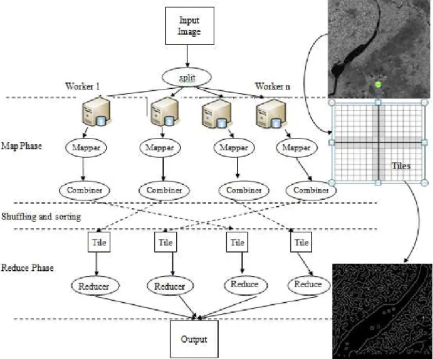
26 Figure 3-1 depicts the major components of the two-stage system processing

structure where the Mappers are applied to all input key-value pairs, which generate processed sub-images of intermediate key-value pairs. Combiner gathers unit images of the same files together and Reducers are applied to merge all images associated with the same key. Between the map and reduce phases there is distributed data sorting. In this scenario the codes of the mappers and reducers along with file format definition are packaged by a driver together with some configuration parameters to produce one MapReduce program where it can be submitted to a master server to process images. There is no direct relationship between the input image files and the MapReduce program and to execute this job the HDFS file path of the image files have to be submitted along with the package to the master. All other aspects of the distributed processing of the images such as distributed execution, failure-handling, job scheduling etc [Venner, 2009]. The following sections discuss in detail about the main components of the MapReduce program.

(41)

27 3.2 Data Input and Output

The image input for our MapReduce job is typically large satellite image files stored in the Hadoop Distributed File System. Our design assumes that these images are stored in tiled TIFF format with augmented metadata where they can be readily read by tiling methods within the boundary of the whole image without restriction. Hadoop provides us with many input and output formats such as text format, binary format, database format etc through the InputFormat

and OutputFormat interfaces [White, 2009]. These interfaces are extendable and therefore we designed our own file format on the top of Hadoop’s

FileInputFormat class that reads image files. This customized FileInputFormat defines from where the input files are to be read by taking the file input path as an argument. It also defines how the input file should be tiled for processing using the IputSplit interface.

The splits do not actually parse and get the tiled data, they are only a reference to the chunk data [White, 2009]. Their primary purpose is how and into how many will the data be sliced. But the actual loading and assigning of keys and values is performed by the RecordReader which is defined by our

(42)

28 Figure 3-2: RasterRecordReader that extends Hadoop's RecordReader interface.

3.3 Data Splitting and Merging

Two kinds of data partitioning mechanisms can be performed on a multispectral data: partition based on the image plane (the spatial domain) or on the spectral space. Partitioning on the spectral space refers to when the input image is portioned based on the spectral bands where the different bands of the same image are to be processed in parallel [Valencia et al., 2008]. While partitioning on the image plane splits the input image into smaller chunks on the spatial domain (in terms of width and height of the image). In this study since the edge detection algorithms are spatial filters that operate on the spatial domain and one band is going to be used independently to enhance edges of the image, we are going to be mainly concerned on how to apply partition of the satellite image on the spatial domain. The performance of parallel implementation of image processing algorithms is highly dependent on how the data is partitioned. One of the key concerns that arise with partitioning images for parallel processing in the spatial domain is the issue of accessing pixels outside the spatial domain of the image splits available in the computing node. This is usually managed by border handling strategy by replication of pixels at the processors to avoid border effects. For instance, if we take the example of Sobel operator which uses 3x3 filtering kernel as a convolution operation, the number of pixels that have to be replicated Pr in the processing of an image can be computed given by the equation below [Valencia et al., 2008].

𝑃𝑃𝑟𝑟 = 2∗ ��2� log2𝑁𝑁

2 � 𝑡𝑡� −1� ∗ 𝐼𝐼𝑅𝑅 + 2∗ ��2� log2𝑁𝑁

(43)

29 Where N is the number of partitions, IR is the number of rows in the original

image, and IC is the number of columns in the original image.

Original Input Image partitioned sub-images

Figure 3-3: Input image splitting strategy to handle border pixels for a 3x3 filter.

The sub-images are generated by splitting the image into regular chunks of the same dimension in horizontal and vertical direction until the end of the whole image. For the Sobel filter which the kernel size is 3x3 a two pixels wide gap forms in the middle of the output image and the outer border pixels are also lost. This is remediated by overlapping the sub-images by two pixels during the slicing of the input image (Figure 3-4). The same strategy must be applied for the 3x3 Laplacian filter. As for the 5x5 Laplacian filter a four pixel overlap was need to remove the pixel gap.

The merging of the of the result images is straight forward as the edge detection algorithms will produce tiles that exactly match at their borders. As outside for the borders of the whole image, they can be ignored if the kernel size is small but for the Canny method where Gaussian smoothing is applied with large kernel sizes (up to 25 pixels width) some mechanism have to be devised to get values for these pixels.

3.4 MapReduce functions

(44)

30 implementing the mapper class. The key-value pairs are the basic data structure

and are the only arguments that the map function needs to start processing (Figure 3-4) [Lin and Dyer, 2010]. The key holds the image file name and the sub-image ID and the value is the sub-image itself. The map function produces an edge detected image as an intermediate value along with the new output keys. In this study the task of the map function is to do the complete edge processing task on the image tiles and give edge image outputs where they are merged by the reduce function. The following sections discuss in detail about the execution overview of the map, reduce, combiner functions and methods involved within these functions.

Figure 3-4: Implements of Mapper and Reducer.

3.4.1 Mapper

It is clear that the map method is a pure function with a sole purpose to process the data splits represented as key-value pairs in parallel mode with no communication with among the other map processes. The map method also receives two more parameters beside the key and value. The first one is the

(45)

31 scenario. The edge detection process is explicitly performed from start to end at

this stage. The sequential implementation of the edge detection algorithms can be easily plugged into the map function with no or slight modifications. The processed images are then compressed into array of bytes where they are represented as key-value pairs and sent to the reducers. When a map task finishes, then the master forward these key-value pairs to the reduce workers. At this stage, in order to reduce the volume of the intermediate images to be transferred to the reduce workers over the network, grouping of the intermediate computed image tiles is made by the map worker nodes locally by the combiner function (similar to the reduce function) which we will discuss it in section 3.3.3. Since a MapReduce job have mappers and reducers running in parallel and sharing the distributed file system, special attention is taken in the file naming system of the intermediate files to avoid conflicts and synchronization between the mappers. The mappers run until all the key-value pairs are processed and after the finishing of all the mappers we can terminate the code and close the data output streaming. Figure 3-5 shows a Unified Modeling Language (UML2) sequence diagram depicting the main execution overview of the map phase. It also shows how the execution framework instantiates the map tasks.

(46)

32 3.4.2 Combiner

To minimize the communication over network during the sorting and shuffling process a combiner function is used to aggregate the image out puts from the mappers locally before being sent to the reduce workers. This combiner function does exactly the same process as the reduce function but only aggregates output image tiles if they are found next to each other in the whole image. This brought a slight challenge to the reduce function as some of the image tiles are now bigger in size but it greatly improves the performance of both the reduce and the shuffle processes. This combiner function is especially important for the canny method because the output tile is much smaller (more than 20% of the original image) than the input tile as it is in binary format.

3.4.3 Reducer

(47)

33 Figure 3-6: Sequence diagram for the reduce phase.

3.5 MapReduce Driver

(48)

34

Chapter 4 Implementation

The Apache Hadoop MapReduce framework is favored as a distributed platform for processing of large remote sensing images because of its simplicity in setup and deployment and its high-level java development tools. The edge diction algorithms are implemented using the apache Hadoop MapReduce framework for as a map and reduce functions. All the development of the algorithms and associated codes are developed in java. By extending the current API in the Hadoop library a system is built that allows for parallel implementation of the image processing algorithms. This chapter discusses the MapReduce implementation details of these algorithms on Apache Hadoop environment.

4.1 Extending Hadoop API

The Hadoop API allows for creation an extension of input formats, by implementing the FileInputFormat and RecordReader interfaces where it becomes possible to describe the way the input image is split and sent to the Mappers for processing. The BytesWritable container of Hadoop API was used in this implementation to allow images to be parsed by the FileInputFormat. The BytesWritable is a wrapper for an array of binary data and its serialized format is an integer field that specifies the number of bytes to follow, followed by the bytes themselves [White, 2009]. Therefore the input image tiles can be easily parsed and wrapped using this container.

First, a class was created that extends the Hadoop RecordReader class to deliver the image file contents as the value of the record. The RecordReader is an important class that is used by the Map function to generate record key-value pairs. This RasterRecordReader inherited class created is also used to generate record key-value pairs for the image splits to be processed by the map function. Since the input images are too big to be read at once for splitting, the Java Advanced Imaging (JAI) API was used to read the image from the file system one image split at a time and convert it into key-value pair format. The ImageReader

(49)

35 (tilePositionX+_tilePositionY+_tileWidth+_tileHeight) which is the key part in the

key-value pair is given to it based on its location in the original image. The process continues to read the next tile until the whole image is tiled. This naming system is crucial for the reduce function which sorts and merge the image tiles together based on this information.

This image splitting method is used inside our extended RasterRecordReader

which is able to split the image convert it to key-value pairs in the form of an array of binary data and make it ready for the map function to process those image split. The main methods that are implemented in this class can be seen in Figure 3-3. It is also here where we define the number of pixel rows and columns that are going to be overlapped among the image tiles depending on which edge detection algorithm is being implemented. The pseudo code in Listing 4-1 shows the important sections of code the adopted image reading and splitting mechanism by the RasterRecordReader. Here, we can observe that the minimum dimension of an image in order to be split is 1024x1024, images below that size are directly converted to key-value pairs.

A second class that is extended in this study is the FileInputFormat (Figure 3-2) which is the base class for any file-based input formats that provides a place to define which files are included as the input to a job and also an implementation for generating splits for the input files [White, 2009]. In our case, both are both these are implemented by the RasterRecordReader class, therefore the main purpose our extension of the FileInputFormat is to the instantiate the

RasterRecordReader. Another important argument is also passed in this implementation: the FileInputFormat also by default splits data that are larger than the HDFS block size. Since we have implemented our own splitting mechanism in the within the RecordReader, any splitting by that might be done by default by FileInputFormat is disabled by overriding the isSplittable()

(50)

36 RecordReader<Text, BytesWritable>

declare variables

overlap; tile width; tile height;

// start the splitting and key-value generation process

initialize(FileSplit, Configuration); getHDFSFilePath();

getFileSystem();

hdfs.open(); //opens HDFS

hdfs.mkdir(hdfs_path+"filename"+"output"); //create directory for tiles

// Split the image only if it is > 1024x1024pixels if( width * height is less greater than 1024*1024 ){ key(filename); &// URI format

value(wholeImage); }

else{ count=0;